Solitons supported by complex PT symmetric Gaussian potentials

Abstract

The existence and stability of fundamental, dipole, and tripole solitons in Kerr nonlinear media with parity-time symmetric Gaussian complex potentials are reported. Fundamental solitons are stable not only in deep potentials but also in shallow potentials. Dipole and tripole solitons are stable only in deep potentials, and tripole solitons are stable in deeper potentials than for dipole solitons. The stable regions of solitons increase with increasing potential depth. The power of solitons increases with increasing propagation constant or decreasing modulation depth of the potentials.

I INTRODUCTION

Quite recently much attention has been paid to light propagation in parity-time (PT) symmetric optical media in theory and experiment PT2010-PRL ; PT2011-oe ; PT2009-PRL ; PT2008-PRL ; PT2010-Nature ; PT2010-pra . This interest was motivated by various areas of physics, including quantum field theory and mathematical physics PT1998-prl ; PT2002-prl ; PT2003-czy ; PT2008-pla ; PT2007-pla ; PT2007-jmp ; PT2005-pla ; PT2000-pla ; PT2005-plb . Quantum mechanics requires that the spectrum of every physical observable quantity is real, thus it must be Hermitian. However, Bender et al pointed out that the non-Hermitian Hamiltonian with PT symmetry can exhibit entirely real spectrum PT1998-prl . Many people discussed the definition of PT symmetric operator and its properties. A Hamiltonian with a complex PT symmetric potential requires that the real part of the potential must be an even function of position, whereas the imaginary part should be odd. It was suggested that in optics the refractive index modulation combined with gain and loss regions can play a role in the complex PT symmetric potential PT2005-ol .

Spatial solitons have been studied since their first theoretical prediction DSs1964-pl . Recently, researchers have focused on composite multimode solitons. Many composite multimode solitons are associated with dipole and tripole solitons. In local Kerr-type media, fundamental solitons are stable, whereas multimode solitons are unstable. Otherwise, multimode solitons have been studied in nonlocal nonlinear media theoretically and experimentally DSs2010-pra ; DSs2007-pra ; DSs2006-ol . Many authors have paid much attention to multimode solitons in optical lattices too DSs2009-pra ; DSs2006-oe ; DSs2010-optik .

In this paper, we find that dipole and tripole solitons can exist and be stable in Kerr nonlinear media with PT symmetric Gaussian complex potentials. The stabilities of fundamental, dipole, and tripole solitons are mainly determined by their corresponding linear modes for low propagation constants or deep potentials. Fundamental solitons are stable not only in deep potentials but also in shallow potentials. But dipole and tripole solitons are only stable in deep potentials, and tripole solitons are stable in potentials deeper than that for dipole solitons. The stable ranges of solitons increase with increasing potential depth.

II MODEL

We consider the (1+1)-dimensional evolution equation of beam propagation along the longitudinal direction $z$ in Kerr-nonlinear media with complex PT potentials,

$$i\frac{\partial U}{\partial z}+\frac{\partial^{2}U}{\partial x^{2}}+T[V(x)+iW(x)]U+\sigma|U|^{2}U=0.$$ (1)

Here $U$ is the complex envelop of slowly varying fields, $x$ is the transverse coordinate, and $z$ is the propagation distance. $V(x)$ and $W(x)$ are the real and imaginary parts of the complex potentials, respectively, and $T$ is the modulation depth. $\sigma=1$ represents the self-focusing propagation, and $\sigma=0$ represents the linear situation. Complex PT symmetric Gaussian potentials are assumed as

$$V(x)=e^{-x^{2}},\,\,\,\,W(x)=W_{0}xe^{-x^{2}},$$ (2)

where $W_{0}$ is the strength of the imaginary part. For complex PT symmetric Gaussian potentials, all eigenvalues are real when the real part of the potentials is stronger than the imaginary, i.e. $W_{0}<1.0$. Otherwise the eigenvalues are mixed for $W_{0}\geq 1.0$ PT2001-Pla .

We search for stationary linear modes and soliton solutions to Eq. (1) in the form $U=f(x)\exp(i\lambda z)$, where $\lambda$ is the propagation constant, and $f(x)$ is the complex function satisfying the equation

$$\lambda f=\frac{\partial^{2}f}{\partial x^{2}}+T[V(x)+iW(x)]f+\sigma|f|^{2}f.$$ (3)

We numerically solve Eq. (3) for different parameters by the modified square-operator method yang-2007 . To examine the stability of solitons in PT Gaussian potentials, we search for perturbed solutions to Eq. (1) in the form

$$U=e^{i\lambda z}\{f(x)+[g(x)-h(x)]e^{\delta z}+[g(x)+h(x)]^{*}e^{\delta^{*}z}\},$$

where $g(x)\ll f(x)$ and $h(x)\ll f(x)$ are the perturbations, and “*” means complex conjugation. Substituting perturbed $U(x,z)$ into Eq. (1), linearizing for $g(x)$ and $h(x)$, the eigenvalue equations about $g(x)$ and $h(x)$ can be derived

$$\delta g= -i[\frac{d^{2}h}{dx^{2}}-\lambda h+TVh-iTWg+2|f|^{2}h$$

$$-\frac{1}{2}(f^{2}-f^{*2})g-\frac{1}{2}(f^{2}+f^{*2})h],$$

$$\delta h= -i[\frac{d^{2}g}{dx^{2}}-\lambda g+TVg-iTWh+2|f|^{2}g$$ (4)

$$+\frac{1}{2}(f^{2}-f^{*2})h+\frac{1}{2}(f^{2}+f^{*2})g].$$

The growth rate $Re(\delta)$ can be obtained numerically by the original-operator iteration method yang-2008 . If $Re(\delta)>0$, solitons are unstable. Otherwise, they are stable.

III Fundamental Solitons

We first investigate fundamental solitons in PT symmetric Gaussian potentials with $W_{0}=0.1$. Figures 1(a)-1(c) show fields of fundamental solitons with different propagation constants and potential depths, which correspond to the cases represented by circles in Fig. 2(a). We can see that all the real parts of fields are even symmetric whereas the imaginary parts are odd symmetric. With increasing propagation constant $\lambda$, the beam width narrows and the beam intensity increases. With increasing potential depth, the beam intensity decreases but the beam width changes little.

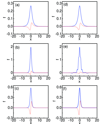
Figure 1: (Color online) Profiles of fundamental solitons with $W_{0}=0.1$ at (a) $T=1$, $\lambda=0.4$; (b)$T=1$, $\lambda=2.6$; and (c)$T=4$, $\lambda=2.6$. (d)-(f) are the linear modes corresponding to (a)-(c), respectively. Solid blue and dotted red lines represent the real and imaginary parts of fields, and imaginary parts are multiplied by 10.

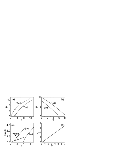
Figure 2: (a) Power $P$ versus propagation constant $\lambda$ with different modulated depths $T$ for fundamental solitons. Solid lines represent stable range and dashed lines represent unstable range. (b Power $P$ versus modulated depth $T$ with different propagation constants $\lambda$ for fundamental solitons. (c) Perturbation growth rate versus propagation constant $\lambda$ with different $T$ values. (d) Critical propagation constant $\lambda_{c}$ versus modulated depth $T$.

Figures 1(d)-1(f) are the field distributions of linear modes corresponding to Figs. 1(a)-1(c), respectively. The field distributions of linear modes and fundamental solitons are homologous for low propagation constants [see Figs. 1(a) and 1(d)], or for deep potentials [Figs. 1(c) and 1(f)], but significantly different for large propagation constants and shallow potentials [Figs. 1(b) and 1(e)]. This phenomenon can be explained qualitatively by Eq. (1). The nonlinear waveguide produced by the term $|U|^{2}U$, along with the real part of the PT potential [$V(x)$], confines the expansion of the beam induced by diffraction, and also suppresses the transverse energy flow induced by the imaginary part of the PT potential [$W(x)$]. Stationary linear modes or solitons are obtained when all these effects are in balance. When the propagation constant is small, the intensity of fundamental solitons and the term $|U|^{2}U$ are small too [see Fig. 2(a)]. The influence of nonlinearity in Eq. (1) is weak, so the field distributions of fundamental solitons are similar to those of corresponding linear modes. The field distributions of linear modes and fundamental solitons are different when the nonlinear term is comparable with the term $V$, i.e., for large propagation constants and shallow potentials [Figs. 1(b) and 1(e)].

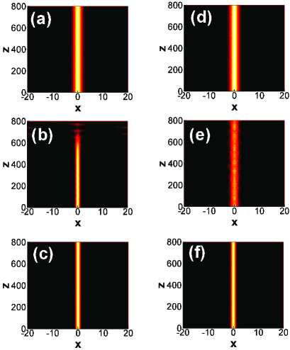
Figure 3: (Color online) (a)-(c): Evolution of fundamental solitons corresponding to Figs. 1(a)-1(c), respectively. (d)-(f): Evolution of fundamental linear modes corresponding to Figs. 1(d)-1(f), respectively.

The power of solitons is defined as $P=\int_{-\infty}^{+\infty}|f(x)|^{2}dx$. Figure 2(a) shows the power of solitons versus the propagation constant $\lambda$ with different $T$ values, and Fig. 2(b) shows the power of solitons versus the potential depth $T$ with different $\lambda$ values. We can see that the power of solitons increases with increasing $\lambda$ or decreasing $T$. Figure 2(c) shows the perturbation growth rate versus the propagation constant $\lambda$ with different $T$ values. One can see that the stable range of fundamental solitons is $\lambda<\lambda_{c}$ for a fixed $T$, where $\lambda_{c}$ is a critical propagation constant for soliton stability. Figure 2(d) shows that $\lambda_{c}$ is approximately proportional to the modulated depth $T$. As $T$ approaches zero, $\lambda_{c}$ approaches zero too, but the value of the growth rate $Re(\delta)$ decreases entirely [see the curve of $Re(\delta)$ for $T=0.01$ in Fig. 2(c)]. When $T=0$, $Re(\delta)=0$ in the whole range, and solitons are always stable. This is consistent with fundamental solitons in pure Kerr nonlinear media always being stable.

To confirm the results of the linear stability analysis, we simulate the soliton propagation based on Eq. (1) with the input condition $U(x,z=0)=f(x)[1+\epsilon\eta(x)]$ by the split-step Fourier method, where $\eta(x)$ is a random function with a value of between $0$ and $1$. $\epsilon$ is a perturbation constant, which is 10 % in our simulation. Figure 3 shows the evolution of beams corresponding to those in Fig. 1, which is in agreement with the stability analysis in Fig. 2. When fundamental solitons are stable, the corresponding linear modes propagate with no distortion [Figs. 3 (d) and 3(f)]. This means that the linear modes absorb the energy of the perturbation noise and maintain its mode profiles. When fundamental solitons are unstable, the corresponding linear modes propagate with random distortions [Fig. 3(e)]. This indicates that the linear modes and perturbation propagate independently without energy exchange. According to Figs. 1 and 3, we can see that the stability of fundamental solitons are mainly decided by the complex potentials for low propagation constants or deep potentials.

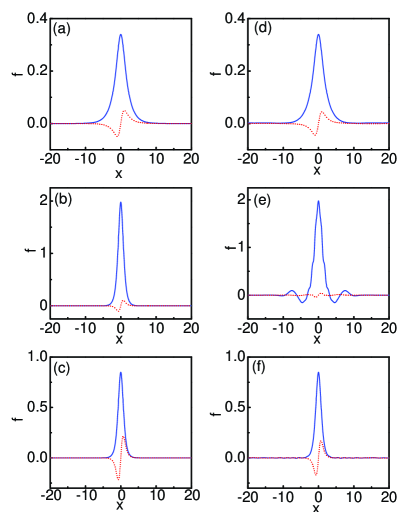
Figure 4: (Color online) Profiles of fundamental solitons with $W_{0}=0.8$ at (a) $T=1$, $\lambda=0.4$; (b)$T=1$, $\lambda=2.6$; and (c)$T=4$, $\lambda=2.6$. (d)-(f) Linear modes corresponding to (a)-(c), respectively. Solid blue and dotted red lines represent real and imaginary parts of fields.

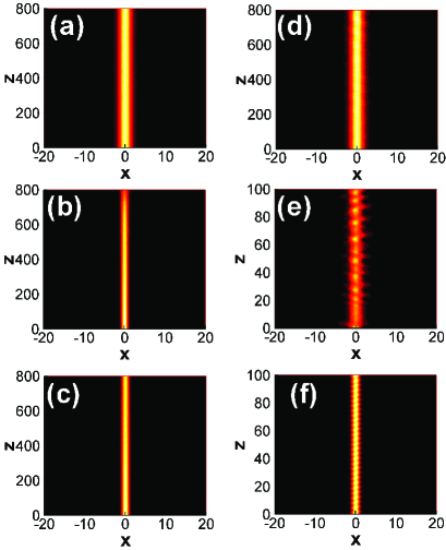
Figure 5: (Color online) (a)-(c): Evolution of fundamental solitons corresponding to Figs. 4(a)-4(c), respectively. (d)-(f): Evolution of fundamental linear modes corresponding to Figs. 4(d)-4(f), respectively.

We also study fundamental solitons in the PT symmetric Gaussian potentials with $W_{0}=0.8$. Figures 4(a)-4(c) show the field distributions of fundamental solitons with different propagation constants and potential depths for $W_{0}=0.8$, whereas Figs. 4(d)-4(f) are the linear modes corresponding to them. We can see that the properties of fundamental solitons for different $W_{0}$ are very similar, except the imaginary parts of fields for $W_{0}=0.8$ are larger than those for $W_{0}=0.1$. Figure 5 shows the beam evolutions corresponding to those in Fig. 4. We can see that fundamental solitons can propagate stably although $W_{0}$ is close to the point of PT breaking [Figs. 5(a) and 5(c)].

IV Dipole and Tripole Solitons

We now investigate dipole solitons in PT symmetric Gaussian potentials with $W_{0}=0.1$. Figures 6(a)-6(c) show the field distributions of dipole solitons, which correspond to the cases represented by circles in Fig. 7(a). Figures 6(d)-6(f) are the linear modes corresponding to Figs. 6(a)-6(c). We can see that all the real parts of the fields are odd symmetrical and the imaginary parts are even symmetrical, which is converse to the situation for fundamental solitons. It is noteworthy that all of the field distributions of linear modes and dipole solitons are similar in Fig. 6. Due to the deep potentials and small propagation constants, the field distributions of solitons are decided mainly by PT symmetric Gaussian complex potentials.

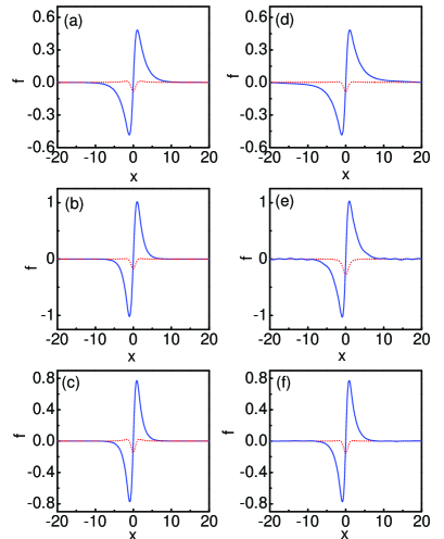
Figure 6: (color online) Profiles of dipole solitons with $W_{0}=0.1$ at (a) $T=4$, $\lambda=0.3$; (b)$T=4$, $\lambda=0.8$; and (c)$T=5$, $\lambda=0.8$. (d)-(f) Linear modes corresponding to (a)-(c), respectively. Solid blue and dotted red lines represent real and imaginary parts of fields, and imaginary parts are multiplied by 2.

The changes in the power versus $\lambda$ and $T$ for dipole solitons are shown in Figs. 7(a) and 7(b), respectively. The power of solitons increases with increasing $\lambda$ or decreasing $T$, which is similar to the situation for fundamental solitons. Figure 7(c) shows the perturbation growth rate versus the propagation constant $\lambda$ for different $T$. Figure 7(d) shows the critical propagation constant $\lambda_{c}$ versus the modulated depth $T$. We can see that dipole solitons exist stably only in deep potentials , i.e. $T\geq 3$, and the stable range increases with increasing modulation depth $T$.

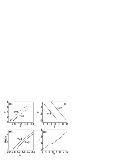
Figure 7: (a) Power $P$ versus propagation constant $\lambda$ with different modulated depths $T$ for dipole solitons; Solid lines represent stable range and dashed lines represent unstable range. (b) Power $P$ versus modulated depth $T$ with different propagation constants $\lambda$ for dipole solitons. (c) Perturbation growth rate versus propagation constant $\lambda$ with different $T$ values. (d) Critical propagation constant $\lambda_{c}$ versus modulated depth $T$.

Dipole solitons are always unstable for $T=0$, which corresponds to pure Kerr nonlinear propagation. A dipole soliton can be considered two solitons with a $\pi$ phase difference, and a repulsive force exists between them. However, we find that the dipole solitons are stable in deep PT symmetric Gaussian potentials. The reason is that the inherent repulsive interaction between solitons can be effectively overcome by the real parts of the complex PT symmetric potentials. This is the reason that dipole solitons are stable only in deep potentials.

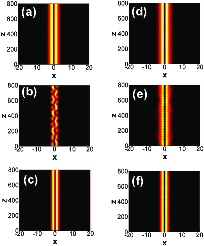
Figure 8: (Color online) (a)-(c): Evolution of dipole solitons corresponding to Figs. 6(a)-6(c), respectively. (d)- (f): Evolution of dipole linear modes corresponding to Figs. 6(d)-6(f), respectively.

Figure 8 shows the beam evolutions corresponding to those in Fig. 6, which is agreement with the stability analysis in Fig. 7. The relations of the propagation between dipole solitons and the corresponding linear modes are similar to those between fundamental solitons and their linear modes.

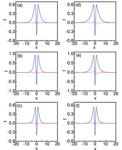
Figure 9: (Color online) Profiles of tripole solitons with $W_{0}=0.1$ at (a) $T=10$, $\lambda=0.3$; (b)$T=10$, $\lambda=0.6$; and (c)$T=12$, $\lambda=0.6$. (d)-(f) Linear modes corresponding to (a)-(c), respectively. Solid blue and dotted red lines represent real and imaginary parts of fields.

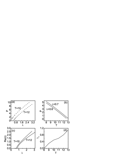
Figure 10: (a) Power $P$ versus propagation constant $\lambda$ with different modulated depths $T$ for tripole solitons. Solid lines represent stable range and dashed lines represent unstable range. (b) Power $P$ versus modulated depth $T$ with different propagation constants $\lambda$ for tripole solitons. (c) Perturbation growth rate versus propagation constant $\lambda$ with different $T$ values. (d) Critical propagation constant $\lambda_{c}$ versus modulated depth $T$.

Finally, we study tripole solitons in PT-invariant Gaussian potentials with $W_{0}=0.1$. Figure 9 shows the field distributions of tripole solitons and their corresponding linear modes, which correspond to the cases represented by circles in Fig. 10(a). We can see that all the real parts of the fields are even symmetrical and the imaginary parts are odd symmetrical, which is similar to the fundamental solitons. Similar to dipole solitons, tripole solitons exist stably in deeper potentials , i.e. $T\geq 8$ [Fig. 10(d)], and all of the field distributions of linear modes and dipole solitons are similar.

The power of solitons increases with increasing $\lambda$ and decreasing $T$, which is similar to fundamental and dipole solitons, as shown in Figs. 10(a) and 10(b). Figure 10(c) shows the perturbation growth rate versus propagation constant and Fig. 10(d) shows the critical propagation constant $\lambda_{c}$ versus modulated depth. We can see that that tripole solitons are stable when $T\geq 8$, which is larger than the value for dipole solitons. The reason is that a tripole soliton can be considered two pairs of out-of-phase solitons, and the repulsive force between them is stronger than that for dipole solitons. Therefore, it needs larger modulation depth $T$ to support tripole solitons than that for dipole solitons.

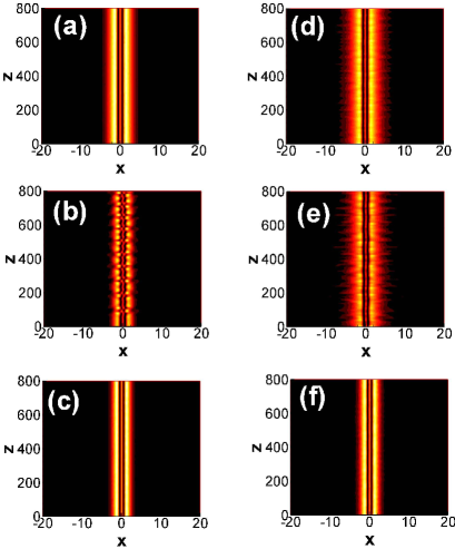
Figure 11: (Color online) (a)-(c): Evolution of tripole solitons corresponding to Figs. 9(a)-9(c), respectively. (d)- (f): Evolution of tripole linear modes corresponding to Figs. 9(d) -9(f), respectively.

Figure 11 shows the beam evolutions corresponding to those in Fig. 9, which are in agreement with the stability analysis in Fig. 10.

V CONCLUSION

In conclusion, we have reported the existence and stability of fundamental, dipole, and tripole solitons supported by Gaussian PT symmetric complex potentials. For monopole fundamental solitons, the waveguide effects from both the nonlinearity and the real part of PT potentials are in balance with the diffraction and the energy flows from the imaginary part of PT potentials. Thus fundamental solitons are stable not only in deep potentials but also in shallow potentials. For multipole solitons, a repulsive force exists between their peaks, which needs a large modulation depth for counterbalance. Therefore multipole solitons exist for a large modulation depth and relatively small propagation constant. Our results may be extended to other PT symmetric optical system, in which multipole solitons can exist.

Our model [Eqs. (1) and (2)] is given in dimensionless form, where $x$ and $z$ are scaled to the potential width $a$ and the diffraction length $L=2k_{0}n_{0}a^{2}$, respectively. Here $k_{0}$ is the wave number in vacuum and $n_{0}$ is the refraction index. $a$ is defined as the half width at the $1/e$ maximum of the real part of PT potentials [see Eq. (2) ], so the full width at half-maximum for $V(x)$ is about $1.665a$ and the extreme of $W(x)$ is located at $\pm 0.707a$. The modulation depth $T$ is scaled to the parameter $1/(2k_{0}^{2}n_{0}a^{2})$. Thus, for a typical waveguide $a=10\mu m$ with the substrate refraction index $n_{0}=3$, the wavelength $\lambda_{0}=1.0\mu$m, and the diffraction length $L=3.77$mm. Then $T=1$ means that the maximum variation of refractive index is $4.22\times 10^{-5}$, and $W=0.1$ means that the maximum gain/loss coefficient is about $0.53{\rm cm}^{-1}$. For these physical parameters, it is feasible to realize multipole solitons in synthetic PT symmetric systems. We hope that the various types of solitons may provide alternative methods in potential applications of synthetic PT symmetric systems.

References

- (1) C. T. West, T. Kottos, and T. Prosen, “PT-Symmetric Wave Chaos,” Phys. Rev. Lett. 104, 054102 (2010).
- (2) H. Wang and J. D. Wang, “Defect solitons in parity-time periodic potentials,” Opt. Express 19, 4030-4035 (2011).
- (3) A. Guo, G. J. Salamo, D. Duchesne, R. Morandotti, M. Volatier-Ravat, V. Aimez, G.A. Siviloglou, and D.N. Christodoulides, “Observation of PT-symmetry Breaking in Complex Optical Potentials,” Phys. Rev. Lett. 103, 093902 (2009).
- (4) Z. H. Musslimani, K. G. Makris, R. El-Ganainy, and D. N. Christodoulides, “Optical solitons in PT periodic potentials,” Phys. Rev. Lett. 100, 030402 (2008).
- (5) C. E. Ruter, K. G. Makris, R. El-Ganainy, D. N. Christodoulides, M. Segev, and D. Kip, ”Observation of parity -time symmetry in optics,” Nature (London)Phys. 6, 192-195 (2010).
- (6) K. G. Makris, R. El-Ganainy, D. N. Christodoulides, and Z. H. Musslimani, “PT-symmetric optical lattices,” Phys. Rev. A81, 063807(2010).
- (7) C. M. Bender and S. Boettcher, “Real spectra in non-hermitian hamiltonians having PT symmetry,” Phys. Rev. Lett. 80, 5243-5246 (1998).
- (8) C. M. Bender, D. C. Brody, and H. F. Jones, “Complex extension of quantum mechanics,” Phys. Rev. Lett. 89, 270401 (2002).
- (9) K. A. Milton, “PT-symmetric quantum field theory,” Czech. J. Phys. 53, 1069-1072 (2003).
- (10) F. Cannata, and A. Ventur, “Overcritical PT -symmetric square well potential in the Dirac equation,” Phys. Lett. A. 372, 941-946 (2008).
- (11) C. S. Jia, J. Y. Liu, P. Q. Wang, and C. S. Chen, “Trapping neutral fermions with a PT-symmetric trigonometric potential in the presence of position-dependent mass,” Phys. Lett. A 369, 274-279 (2007).
- (12) C. M. Bender, S. Boettcher, and P. N. Meisinger, “PT-symmetric quantum mechanics,” J. Math. Phys. 40, 2201 (1999).
- (13) H. Egrifes and R. Sever, “Bound states of the Dirac equation for the PT-symmetric generalized Hulth n potential by the Nikiforov-Uvarov method,” Phys. Lett. A 344, 117-126 (2005).
- (14) B. Bagchi, F. Cannata, and C. Quesne, ”PT-symmetric sextic potentials,” Phys. Lett. A 269, 79-82 (2000).
- (15) C. M. Bender , H. F. Jones , and R. J. Rivers, “Dual PT -symmetric quantum field theories,” Phys. Lett. B 625, 333-340 (2005).
- (16) S. V. Dmitriev, A. A. Sukhorukov, and Y. S. Kivshar, “Binary parity-time-symmetric nonlinear latticeswith balanced gain and loss,” Opt. Lett. 35, 2976-2978 (2005).
- (17) R. Y. Chiao, E. Garmire, and C. H. Townes, “Self-trapping of optical beam,” Phys. Lett. 13, 479-484 (1964).
- (18) L. W. Dong and F. W. Ye, “Stability of multipole-mode solitons in thermal nonlinear media,” Phys. Rev. A81, 013815 (2010).
- (19) V. M. Lashkin, “Two-dimensional nonlocal vortices, multipole solitons, and rotating multisolitons in dipolar Bose-Einstein condensates,” Phys. Rev. A75, 043607 (2007).
- (20) Z. Y. Xu, Y. V. Kartashov, and M. Segiv, “Two-dimensional multipole solitons in nonlocal nonlinear media,” Opt. Lett. 31, 3312-3314 (2006).
- (21) Z. Y. Xu, “Multipole-mode interface solitons in quadratic nonlinear photonic lattices,” Phys. Rev. A80, 053827 (2009).
- (22) Y. J. He, and H. Z. Wang, “(1+1)-dimensional dipole solitons supported by optical latice,” Opt. Express 14, 9832-9837 (2006).
- (23) X. L. Wu and R. C. Yang, “Diploe solitons in an optical lattice with longitudinal modulation,” Optik 121, 1466-1471 (2010).
- (24) Z. Ahmed, “Real and complex discrete eigenvalues in an exactly solvable one-dimensional complex PT-invariant potential,” Phys. Lett. A 282, 343-348 (2001).
- (25) J. Yang, and T. I. Lakoba, Stud. Appl. Math. 118, 153-197 (2007).
- (26) J. Yang, J. Comput. Phys. 227, 6862-6876 (2008).