Motion Planning via Manifold Samples

Abstract

We present a general and modular algorithmic framework for path planning of robots. Our framework combines geometric methods for exact and complete analysis of low-dimensional configuration spaces, together with practical, considerably simpler sampling-based approaches that are appropriate for higher dimensions. In order to facilitate the transfer of advanced geometric algorithms into practical use, we suggest taking samples that are entire low-dimensional manifolds of the configuration space that capture the connectivity of the configuration space much better than isolated point samples. Geometric algorithms for analysis of low-dimensional manifolds then provide powerful primitive operations. The modular design of the framework enables independent optimization of each modular component. Indeed, we have developed, implemented and optimized a primitive operation for complete and exact combinatorial analysis of a certain set of manifolds, using arrangements of curves of rational functions and concepts of generic programming. This in turn enabled us to implement our framework for the concrete case of a polygonal robot translating and rotating amidst polygonal obstacles. We demonstrate that the integration of several carefully engineered components leads to significant speedup over the popular PRM sampling-based algorithm, which represents the more simplistic approach that is prevalent in practice. We foresee possible extensions of our framework to solving high-dimensional problems beyond motion planning.

1 Introduction

Motion planning is a fundamental research topic in robotics with applications in diverse domains such as graphical animation, surgical planning, computational biology and computer games. For a general overview of the subject and its applications see [10, 21, 23]. In its basic form, the motion-planning problem is to find a collision-free path for a robot or a moving object $R$ in a workspace cluttered with static obstacles. The spatial pose of $R$, or the configuration of $R$, is uniquely defined by some set of parameters, the degrees of freedom (dofs) of $R$. The set of all robot configurations $\mathcal{C}$ is termed the configuration space of the robot, and decomposes into the disjoint sets of free and forbidden configurations, namely $\mathcal{C}_{\rm free}$ and $\mathcal{C}_{\rm forb}$, respectively. Thus, it is common to rephrase the motion-planning problem as the problem of moving $R$ from a start configuration $q_{s}$ to a target configuration $q_{t}$ in a path that is fully contained within $\mathcal{C}_{\rm free}$.

Analytic solutions to the general motion planning problem: The motion-planning problem is computationally hard with respect to the number of dofs [28], yet much research has been devoted to solving the general problem and its various instances using geometric, algebraic and combinatorial tools. The configuration-space formalism was introduced by Lozano-Perez [25] in the early 1980’s. Schwartz and Sharir proposed the first general algorithm for solving the motion planning problem, with running time that is doubly-exponential in the number of dofs [30]. Singly exponential-time algorithms have followed [4, 8, 9], but are generally considered too complicated to be implemented in practice.

Solutions to low-dimensional instances of the problem: Although the general motion-planning problem cannot be efficiently solved analytically, more efficient algorithms have been proposed for various low-dimensional instances [21], such as translating a polygonal or polyhedral robot [1, 25], and translation with rotation of a polygonal robot in the plane [3, 14, 29]. For a survey of related approaches see [31]. Moreover, considerable advances in robust implementation of computational geometry algorithms in recent years have led to a set of implemented tools that are of interest in this context. Minkowski sums, which allow representation of the configuration space of a translating robot, have robust and exact planar and 3-dimensional implementations [12, 13, 34]. Likewise, implementations of planar arrangements for curves  [33, C.30], are essential components in [30].

Sampling-based approaches to motion planning: The sampling-based approach to motion-planning has extended the applicability of motion planning algorithms beyond the restricted subset of problems that can be solved efficiently by exact algorithms [10, 23]. Sampling-based motion planning algorithms, such as Probabilistic Roadmaps (PRM) [18], Expansive Space Trees (EST) [16] and Rapidly-exploring Random Trees (RRT) [22], as well as their many variants, aim to capture the connectivity of $\mathcal{C}_{\rm free}$ in a graph data structure, via random sampling of robot configurations. This can be done either in a multi-query setting, to efficiently answer multiple queries for the same scenario, as in the PRM algorithm, or in a single-query setting, as in the RRT and EST algorithms. For a general survey on the field see [10]. Importantly, the PRM and RRT algorithms were both shown to be probabilistically complete [17, 19, 20], that is, they are guaranteed to find a valid solution, if one exists. However, the required running time for finding such a solution cannot be computed for new queries at run-time, and the proper usage of sampling-based approaches may still be considered somewhat of an art. Moreover, sampling-based methods are also considered sensitive to tight passages in the configuration space, due to the high-probability of missing the passage.

Hybrid methods for motion-planning: Few hybrid methods attempt to combine both deterministic and probabilistic planning strategies. Hirsch and Halperin [15] studied two-disc motion planning by exactly decomposing the configuration space of each robot, then combining the two solutions to a set of free, forbidden and mixed cells, and using PRM to construct the final connectivity graph. Zhang et al. [36] used PRM in conjunction with approximate cell decomposition, which also divides space to free, forbidden and mixed cells. Other studies have suggested to connect a dense set of near-by configuration space “slices”. Each slice is decomposed to free and forbidden cells, but adjacent slices are connected in an inexact manner, by e.g., identifying overlaps between adjacent slices [11, pp. 283-287], or heuristic interpolation and local-planning [24]. In [35] a 6 dof RRT planner is presented with a 3 dof local planner hybridizing probabilistic, heuristic and deterministic methods.

1.1 Contribution

In this study, we present a novel general scheme for motion planing via manifold samples (MMS), which extends sampling-based techniques like PRM as follows: Instead of sampling isolated robot configurations, we sample entire low-dimensional manifolds, which can be analyzed by complete and exact methods for decomposing space. This yields an explicit representation of maximal connected patches of free configurations on each manifold, and provides a much better coverage of the configuration space compared to isolated point samples. At the same time, the manifold samples are deliberately chosen such that they are likely to intersect each other, which allows to establish connections among different manifolds. The general scheme of MMS is illustrated in Figure 1. A detailed discussion of the scheme is presented in Section 2.

In Section 3, we discuss the application of MMS to the concrete case of a polygonal robot translating and rotating in the plane amidst polygonal obstacles. We present in detail appropriate families of manifolds as well as filtering schemes that should also be of interest for other scenarios. Although our software is prototypical, we emphasize that the achieved results are due to careful design and implementation on all levels. In particular, in Section 4 we present an exact analytic solution and efficient implementation to a motion planning problem instance: moving a polygonal robot in the plane with rotation and translation along an arbitrary axis. To the best of our knowledge the problem has not been analytically studied before. The implementation involves advanced algebraic and extension of state-of-the-art applied geometry tools. In Section 5 we present experimental results, which show our method’s superior behavior for several test cases vis-à-vis a common implementation of the sampling-based PRM algorithm. For example, in a tight passage scenario we demonstrate a 27-fold improvement. We conclude with a discussion of extensions of our scheme, which we anticipate could greatly widen the scope of applicability of sampling-based methods for motion planning by combining them with strong analytic tools in a straightforward manner.

2 General Scheme for Planning with Manifold Samples

Preprocessing—Constructing connectivity graph: We propose a multi-query planner for motion planning problems in a possibly high-dimensional configuration space. The preprocessing stage constructs the connectivity graph of $\mathcal{C}$, a data structure that captures the connectivity of $\mathcal{C}$ using manifolds as samples. The manifolds are decomposed into cells in $\mathcal{C}_{\rm free}$ and $\mathcal{C}_{\rm forb}$ in a complete and exact manner; we call a cell of the decomposed manifold that lies in $\mathcal{C}_{\rm free}$ a free space cell ($F\!\!\>S\!\!\>C$) and refer to the connectivity graph as $\mathcal{G}$. The $F\!\!\>S\!\!\>Cs$ serve as nodes in $\mathcal{G}$ while two nodes in $\mathcal{G}$ are connected by an edge if their corresponding $F\!\!\>S\!\!\>Cs$ intersect. See Figure 1 for an illustration

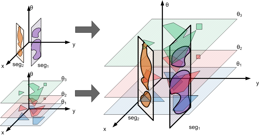
Figure 1: Three-dimensional configuration space: The left side illustrates two families of manifolds where the decomposed cells are darkly shaded. The right side illustrates their intersection that induces the graph $\mathcal{G}$.

We formalize the preprocessing stage by considering manifolds induced by a family of constraints $\Psi$, such that $\psi\in\Psi$ defines a manifold $m_{\psi}$ of the configuration space. The construction of a manifold $m_{\psi}$ and its decomposition into $F\!\!\>S\!\!\>Cs$ are carried out via a $\Psi$-primitive (denoted $P_{\Psi}$) applied to an element $\psi\in\Psi$. By a slight abuse of notations we refer to an $F\!\!\>S\!\!\>C$ both as a cell and a node in the graph. Using this notation, Algorithm 1 summarizes the construction of $\mathcal{G}$. In lines 3-4, a new manifold constraint is generated and added to the collection of manifold constraints $X$. In lines 5-7, the manifold induced by the new constraint is decomposed by the appropriate primitive and its $F\!\!\>S\!\!\>Cs$ are added to $\mathcal{G}$.

Algorithm 1 Construct Connectivity Graph

1:  $V\leftarrow\emptyset$, $E\leftarrow\emptyset$, $X\leftarrow\emptyset$

2:  repeat

3:     $\psi\leftarrow$ generate_constraint($V$,$E$,$X$)

4:     $X\leftarrow X\cup\{\psi\}$

5:     $F\!\!\>S\!\!\>C_{m_{\psi}}\leftarrow P_{\Psi}(m_{\psi})$

6:     $V\leftarrow V\cup\{$fsc$|\$fsc$\in F\!\!\>S\!\!\>C_{m_{\psi}}\}$

7:     $E\leftarrow E\cup\{($fsc${}_{1},$ fsc${}_{2})\ |$   fsc${}_{1}\in V,$ fsc${}_{2}\in F\!\!\>S\!\!\>C_{m_{\psi}}$ ,                              fsc${}_{1}\cap$fsc${}_{2}\neq\emptyset\$ & fsc${}_{1}\neq$fsc${}_{2}\}$

8:  until stopping_condition

9:  return  $G(V,E)$

Query: Once the connectivity graph $\mathcal{G}$ has been constructed it can be queried for paths between two configurations $q_{s}$ and $q_{t}$ in the following manner: A manifold that contains $q_{s}$ (respectively $q_{t}$) in one of its $F\!\!\>S\!\!\>Cs$ is generated and decomposed. Its $F\!\!\>S\!\!\>Cs$ and their appropriate edges are added to $\mathcal{G}$. We compute a path $p$ in $\mathcal{G}$ between the $F\!\!\>S\!\!\>Cs$ that contain $q_{s}$ and $q_{t}$. A path in $\mathcal{C}_{\rm free}$ may then be computed by planning a path within each $F\!\!\>S\!\!\>C$ in $p$.

2.1 Desirable Properties of Manifold Families

Choosing the specific set of manifold families may depend on the concrete problem at hand, as detailed in the next section. However, it seems desirable to retain some general properties. First, each manifold should be simple enough such that it is possible to decompose it into free and forbidden cells in a computationally effcient manner. The choice of manifold families should also cover the configuration space, such that each configuration intersects at least a single manifold $m_{\psi}$. In addition, local transitions between close-by configurations should be made possible via cross-connections of several intersecting manifolds, which we term the spanning property. We anticipate that these simple and intuitive properties (perhaps subject to some fine tuning) may lead to a proof of probabilistic completeness of the approach.

2.2 Exploration and Connection Strategies

A naïve way to generate constraints that induce manifolds is by random sampling. Primitives may be computationally complex and should thus be applied sparingly. We suggest a general exploration/connection scheme and additional optimization heuristics that may be used in concrete implementations of the proposed general scheme. We describe strategies in general terms, providing conceptual guidelines for concrete implementations, as demonstrated in Section 3.

Exploration and connection phases: Generation of constraints is done in two phases: exploration and connection. In the exploration phase constraints are generated such that primitives will produce $F\!\!\>S\!\!\>Cs$ that introduce new connected components in $\mathcal{C}_{\rm free}$. The aim of the exploration phase is to increase the coverage of the configuration space as efficiently as possible. In contrast, in the connection phase constraints are generated such that primitives will produce $F\!\!\>S\!\!\>Cs$ that connect existing connected components in $\mathcal{G}$. Once a constraint is generated, $\mathcal{G}$ is updated as described above. Finally, we note that we can alternate between exploration and connection, namely we can decide to further explore after some connection work has been performed.

Region of interest (RoI): Decomposing an entire manifold $m_{\psi}$ by a primitive $P_{\Psi}$ may be unnecessary. Patches of $m_{\psi}$ may intersect $\mathcal{C}_{\rm free}$ in highly explored parts or connect already well-connected parts of $\mathcal{G}$ while others may intersect $\mathcal{C}_{\rm free}$ in sparsely explored areas or less well connected parts of $\mathcal{G}$. Identifying the regions where the manifold is of good use (depending on the phase) and constructing $m_{\psi}$ only in those regions increases the effectiveness of $P_{\Psi}$ while desirably biasing the samples. We refer to a manifold patch that is relevant in a specific phase as the Region of Interest - RoI of the manifold.

Constraint filtering Let $\psi\in\Psi$ be a constraint such that applying $P_{\Psi}$ to $\psi$ yields the set of $F\!\!\>S\!\!\>Cs$ on $m_{\psi}$. If we are in the connection phase, inserting the associated nodes into $\mathcal{G}$ and intersecting them with the existing $F\!\!\>S\!\!\>Cs$ should connect existing connected components of $\mathcal{G}$. Otherwise, the primitive’s contribution is poor. We suggest applying a filtering predicate immediately after generating a constraint $\psi$ to check if $P_{\Psi}(\psi)$ may connect existing connected components of $\mathcal{G}$. If not, the primitive should not be constructed and $\psi$ should be discarded.

3 The Case of Rigid Polygonal Motion

We demonstrate the scheme suggested in Section 2 by considering a polygonal robot $R$ translating and rotating in the plane amidst polygonal obstacles. A configuration of $R$ describes the position of the reference point (center of mass) of $R$ and the orientation of $R$. As we consider full rotations, the configuration space $\mathcal{C}$ is the three dimensional space $\mathbb{R}^{2}\times S^{1}$.

3.1 Manifold Families

As defined in Section 2, we consider manifolds defined by constraints and construct and decompose them using primitives. We suggest the following constraints restricting motions of $R$ and describe their associated primitives: The Angle Constraint fixes the orientation of $R$ while it is still free to translate anywhere within the workspace; the Segment Constraint restricts the position of the reference point to a segment in the workspace while $R$ is free to rotate.

The left part of Figure 1 demonstrates decomposed manifolds associated to the angle (left bottom) and segment (left top) constraints. The angle constraint induces a two-dimensional horizontal plane where the cells are polygons. The segment constraint induces a two-dimensional vertical slab where the cells are defined by the intersection of rational curves (as explained in Section 4).

We delay the discussion of creating and decomposing manifolds to Section 4. For now, notice that the Segment-Primitive is far more time-consuming than the Angle-Primitive.

3.2 Exploration and Connection Strategies

We use manifolds constructed by the Angle-Primitive for the exploration phase and manifolds constructed by the Segment-Primitive for the connection phase. Since the Segment-Primitive is far more costly than the Angle-Primitive, we focused our efforts on optimizing the former.

Region of interest - RoI: As suggested in Section 2.2 we may consider the Segment-Primitive in a subset of the range of angles. This results in a somewhat “weaker” yet more efficient primitive than considering the whole range. If the connectivity of a local area of the configuration space is desired, then using this optimization may suffice while considerably speeding up the algorithm.

Generating segments: Consecutive layers (manifolds of the Angle Constraint) have a similar structure unless topological criticalities occur in $\mathcal{C}$. Once a topological criticality occurs, an $F\!\!\>S\!\!\>C$ either appears and grows or shrinks and disappears. We thus suggest a heuristic for generating a segment in the workspace for the Segment-Primitive using the size of the cell as a parameter where we refer to small and large cells according to pre-defined constants. The RoI used will be proportional to the size of the $F\!\!\>S\!\!\>C$. The segment generated will be chosen with one of the following procedures which are used in Algorithm 2.

Random procedure: Return a random segment from the workspace.

Large cell procedure: Return a random segment in the cell.

Small cell procedure: Intersect the $F\!\!\>S\!\!\>C$ with the next (or the previous) layer. Return a segment connecting a random point from the $F\!\!\>S\!\!\>C$ and a random point in the intersection.

Algorithm 2 Generate Segment Constraint ($V$,$E$)

1:  if random_num ($[0,1])\geq$ random_threshold then

2:     return  random_segment_procedure()

3:  else

4:     fsc $\leftarrow$ random_fsc(V)

5:     $\alpha\leftarrow$ [size(fsc) - small_cell_size] / [large_cell_size - small_cell_size]

6:     if random_num($[0,1])\geq\alpha$ then

7:        return  small_cell_procedure(fsc,$V$)

8:     else

9:        return  large_cell_procedure(fsc,$V$)

10:     end if

11:  end if

Constraint Filtering: As suggested in Section 2.2, we avoid computing unnecessary primitives. All $F\!\!\>S\!\!\>Cs$ that will intersect a “candidate” constraint $s$, namely all $F\!\!\>S\!\!\>Cs$ of layers in its RoI, are tested. If they are all in the same connected component in $\mathcal{G}$, $s$ can be discarded as demonstrated in Algorithm 3.

Algorithm 3 Filter Segment ($s$,$RoI$,$V$,$E$)

1:  $cc_{ids}\leftarrow\emptyset$

2:  for all $v\in V$ do

3:     fsc $\leftarrow$ free_space_cell($v$)

4:     if constraining_angle(fsc)$\in RoI$ then

5:        $cc_{ids}\leftarrow cc_{ids}\cup$ connected_component_id($v$)

6:     end if

7:  end for

8:  if $|cc_{ids}|\leq 1$ then

9:     return  filter_out

10:  end if

3.3 Path Planning Query

For a query $q=(q_{s},q_{t})$, where $q_{s}=(x_{s},y_{s},\theta_{s})$ and $q_{t}=(x_{t},y_{t},\theta_{t})$, $P_{\Theta}(\theta_{s})$ and $P_{\Theta}(\theta_{t})$ are constructed and the $F\!\!\>S\!\!\>Cs$ are added to $\mathcal{G}$. A path of $F\!\!\>S\!\!\>Cs$ between the $F\!\!\>S\!\!\>Cs$ containing $q_{s}$ and $q_{t}$ is searched for. A local path in an Angle-Primitive’s $F\!\!\>S\!\!\>C$ (which is a polygon) is constructed by computing the shortest path on the visibility graph defined by the vertices of the polygon. A local path in an $F\!\!\>S\!\!\>C$ of a Segment-Primitive (which is an arrangement cell) is constructed by applying cell decomposition and computing the shortest path on the graph induced by the decomposed cells. (Figure 5 depicts a path in a segment manifold.)

4 Efficient Implementation of Manifold Decomposition

The algorithm discussed in Section 3 is implemented in C++. It is based on Cgal’s arrangement package, which is used for the geometric primitives, and the Boost graph library [32], which is used to represent the connectivity graph $\mathcal{G}$. We next discuss the manifold decomposition methods in more detail.

Angle-Primitive: The Angle-Primitive for a constraining angle $\theta$ (denoted $P_{\Theta}(\theta)$) is constructed by computing the Minkowski sum of $-R_{\theta}$ with the obstacles. The implementation is an application of Cgal’s Minkowski sums package [33, C.24]. We remark that we ensure (using the method of Canny et al. [7]) that the angle $\theta$ is chosen such that $\sin\theta$ and $\cos\theta$ are rational. This allows for an exact rotation of the robot and an exact computation of the Minkowski Sum.

Segment-Primitive: Limiting the possible positions of the robot’s reference point $r$ to a given segment $s$, results in a two-dimensional configuration space. Each vertex (or edge) of the robot in combination with each edge (or vertex) of an obstacle gives rise to a critical curve in this configuration space. Namely the set of all configurations that put the two features into contact, and thus mark a potential transition between $\mathcal{C}_{\rm forb}$ and $\mathcal{C}_{\rm free}$. Our analysis (Appendix 0.B) shows that these critical curves can be expressed by rational functions only. Thus, the implementation of the Segment-Primitive is first of all a computation of an arrangement of rational functions.

Cgal follows the generic programming paradigm [2], that is, algorithms are formulated and implemented such that they abstract away from the actual types, constructions and predicates. Using the C++ programming language this is realized by means of class and function templates, respectively. In particular, the arrangement package is written such that it takes a traits class as a template argument. This traits class defines the supported curve type and provides the operations that are required for this type. Since the old specialized traits class was too slow (even slower than the solution for general algebraic curves presented in [6]), we devised a new efficient traits class for rational functions.

The new traits class (all details in Appendix 0.A) is written such that it takes maximal advantage of the fact that the supported curves are functions. As opposed to the general traits in [6], we never have to shear the coordinate system and we only require tools provided by the univariate algebraic kernel of Cgal [33, C.8]. A comparison using the benchmark instances that were also used in [6] shows that the new traits class is about 3-4 times faster then the general traits class; this is a total speed up of about 10 when compared to the old dedicated traits class.

The development of this new traits class represents the low tier of our efforts to produce an effective motion planner and relies on a more intimate acquaintance with Cgal in general and arrangement traits for algebraic curves in particular; therefore we defer further details to the appendix. We note that the new traits class has been accepted for integration into Cgal and will be available in the upcoming Cgal release 3.9.

5 Experimental Results

We demonstrate the performance of our planner using three different scenarios. All scenarios consist of a workspace, a robot with obstacles and one query (source and target configurations). Figure 2 illustrates the scenarios where the obstacles are drawn in blue and the source and target configurations are drawn in green and red, respectively. All reported tests were measured on a Dell 1440 with one 2.4GHz P8600 Intel Core 2 Duo CPU processor and 3GB of memory running with a Windows 7 32-bit OS. Preprocessing times presented are times that yielded at least 80% (minimum of 5 runs) success rate in solving queries.

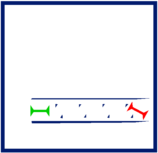
(a) Tunnel scenario

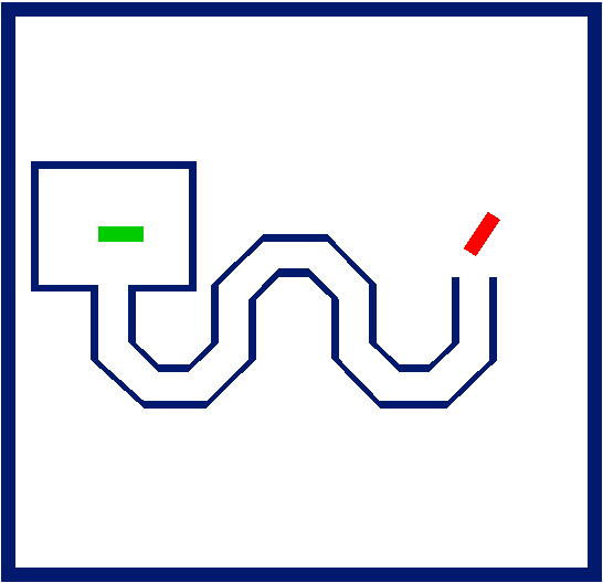
(b) Snake scenario

(c) Flower scenario

Figure 2: Experimental scenarios

5.1 Algorithm Properties

Our planner has two parameters: the number $n_{\theta}$ of layers to be generated and the number $n_{s}$ of segment constraints to be generated. We chose the following values for these parameters: $n_{\theta}\in\{10,20,40,80\}$ and $n_{s}\in\{2^{i}|i\in\mathbb{N},i\leq 14\}$. For a set of parameters $(n_{\theta},n_{s})$ we report the preprocessing time $t$ and whether a path was found (marked ✓) or not found (marked $\times$) once the query was issued. The results for the flower scenario are reported in Table 2. We show that a considerable increase in parameters has only a limited effect on the preprocessing time.

In order to test the effectiveness of our optimizations, we ran the planner with and without any heuristic for choosing segments and with and without segment filtering. We also added a test with all optimizations using the old traits class. The results for the flower scenario can be viewed in Table 2. We remark that the engineering work invested in optimizing MMS yielded an algorithm comparable and even surpassing a motion planner that is in prevalent use as shown next.

		$n_{\theta}$
		10	20	40	80
$n_{s}$	256	(6,$\times$)	(11,$\times$)	(12,$\times$)	(16,$\times$)
	512	(7,$\times$)	(13,$\times$)	(14,$\times$)	(25,$\times$)
	1024	(16,$\times$)	(20,✓)	(23,✓)	(35,✓)
	2048	(30,$\times$)	(35,✓)	(38,✓)	(51,✓)
	4096	(46,✓)	(53,✓)	(60,✓)	(82,✓)

Table 1: Parameter sensitivity

	Segment
Traits	Generation	Filtering	$n_{\theta}$	$n_{s}$	t
New	random	not used	20	8192	1418
		used	20	8192	112
	heuristic	not used	40	512	103
		used	20	1024	20
Old	heuristic	used	20	1024	138

Table 2: Optimization results

5.2 Comparison With PRM

We used an implementation of the PRM algorithm as provided by the OOPSMP package [27]. For fair comparison, we did not use cycles in the roadmap as cycles increase the preprocessing time significantly. We manually optimized the parameters of each planner over a concrete set. As with previous tests, the parameters for MMS are $n_{\theta}$ and $n_{s}$. The parameters used for the PRM are the number of neighbors (denoted $k$) to which each milestone should be connected and the percentage of time used to sample new milestones (denoted % st in Table 4).

Furthermore, we ran the flower scenario several times, progressively increasing the robot size. This caused a “tightening” of the passages containing the desired path. Figure 4 demonstrates the preprocessing time as a function of the tightness of the problem for both planners. A tightness of zero denotes the base scenario (Figure 2c) while a tightness of one denotes the tightest problem solved.

The results show a speedup for all scenarios when compared to the PRM implementation. Moreover, our algorithm has little sensitivity to the tightness of the problem as opposed to the PRM algorithm. In the tightest experiment, MMS runs 27 times faster than the PRM implementation.

Scenario	MMS			PRM			Speedup
	$n_{\theta}$	$n_{s}$	t	k	% st	t
Tunnel	20	512	100	20	0.0125	180	1.8
Snake	40	256	22	20	0.025	140	6.3
Flower	20	1024	20	24	0.0125	40	2

Figure 3: Comparison With PRM

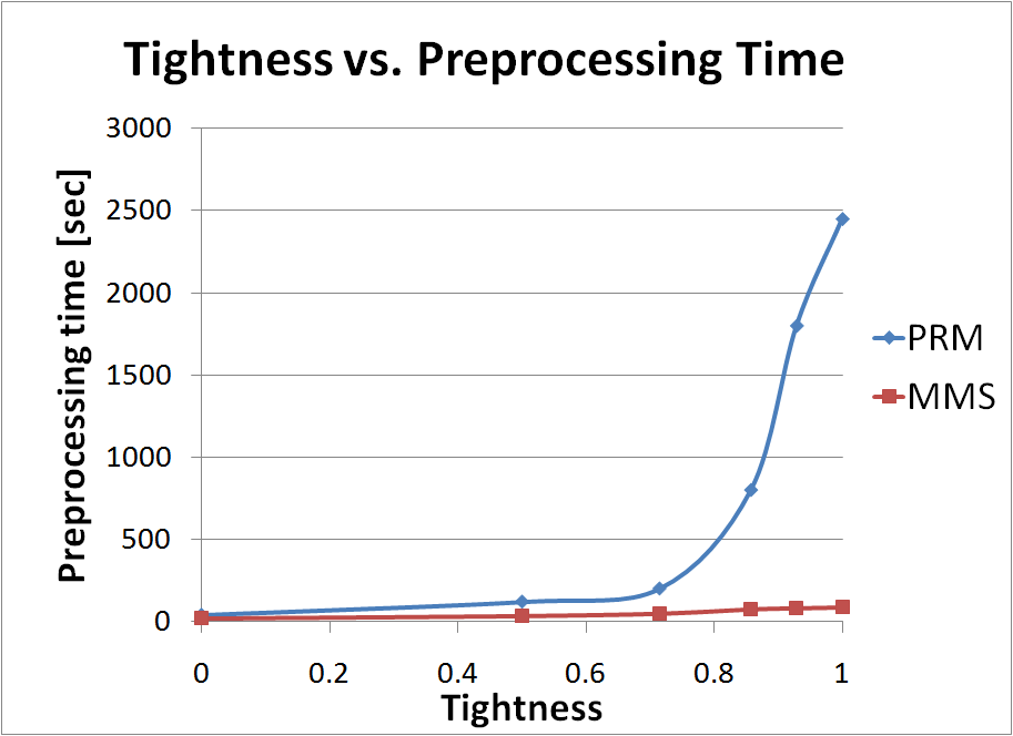
Figure 4: Tightness Results

6 Further Directions

To conclude, we outline directions for extending and enhancing the current work. Our primary goal is to use the MMS framework to solve progressively more complicated motion-planning problems. As suggested earlier, we see the framework as a platform for convenient transfer of strong geometric primitives into motion planning algorithms. For example, among the recently developed tools are efficient and exact solutions for computing the Minkowski sums of polytopes in $\mathbb{R}^{3}$ (see Introduction) as well as for exact update of the sum when the polytopes rotate [26]. These could be combined into an MMS for planning full rigid motion of a polytope among polytopes, which, extrapolating from the current experiments could outperform more simplistic solutions in existence.

Looking at more intricate problems, we anticipate some difficulty in turning constraints into manifolds that can be exactly decomposed. We propose to have manifolds where the decomposition yields some approximation of the $F\!\!\>S\!\!\>Cs$, using recent advanced meshing tools for example. We can endow the connectivity-graph nodes with an attribute describing their approximation quality. One can then decide to only look for paths all whose nodes are above a certain approximation quality. Alternatively, one can extract any solution path and then refine only those portions of the path that are below a certain quality.

Beyond motion planning: We foresee an extension of the framework to other problems that involve high-dimensional arrangements of critical hypersurfaces. It is difficult to describe the entire arrangement analytically, but there are often situations where constraint manifolds could be computed analytically. Hence, it is possible to shed light on problems such as loop closure and assembly planning where we can use manifold samples to analytically capture pertinent information of high-dimensional arrangements of hypersurfaces. Notice that although in Section 3 we used only planar manifolds, there are recently developed tools to construct two dimensional arrangement of curves on curved surfaces [5] which gives further flexibility in choosing the manifold families.

For supplementary material and updates the reader is referred to our webpage http://acg.cs.tau.ac.il/projects/mms.

Appendix 0.A Traits Class for Rational Functions

For completeness we repeat below (in Section 0.A.1) material that already appears in the body of the paper. More technical details on the implementation of the traits class are given in Section 0.A.2.

0.A.1 Background

Cgal follows the generic programming paradigm [2], that is, algorithms are formulated and implemented such that they abstract away from the actual types, constructions, and predicates. Using the C++ programming language this is realized by means of class and function templates, respectively. The manifold decomposition methods described below use Cgal’s arrangement package.

As most other high level packages of Cgal, the arrangement package is written such that it takes one traits class as a template argument. This traits class defines the type of curves in use and the required operations on them. This gives tremendous flexibility in using the package for a variety of different motion planning (sub)problems. Here we use it once for line segments via the Minkowski sums package written on top of the arrangement package, and once with graphs of rational functions, for which we devised a new and particularly efficient traits class. The following section gives more detail about the later.

The new traits class is written such that it takes maximal advantage of the fact that the supported curves are functions. This implies that, as opposed to the general traits in [6], we never have to shear the coordinate system and that we only require tools provided by the univariate algebraic kernel [33, C.8].

A traits class is required to provide (and by that define) the curve type in use. For these curves it must provide a specific set of operations, such as splitting curves into $x$-monotone sub-curves, computing the intersections of two curve segments, comparing intersection points, or comparing the $y$-order of two curves at a certain $x$-coordinate. Thus, our traits class implements these predefined operations explicitly for rational functions. The heart of the traits consists of two classes that represent the complete topology of one or two functions, respectively. All predicates and constructions required for the traits are essentially just queries to one of these two classes.

0.A.2 Technical Details

For one function $f(x)=f_{n}(x)/f_{d}(x)$, with $f_{n},f_{d}\in\mathbb{Z}[X]$ coprime, we subdivide the $x$-axis into intervals such that the sign of $f$ is invariant within each interval. This is obtained by computing the sorted sequence of the real roots (with multiplicity) of $f_{n}$ and $f_{d}$. For the right-most interval the sign is determined by the signs of the leading coefficients of $f_{n}$ and $f_{d}$. The remaining signs are concluded from right to left using the multiplicity of the computed roots.

For two functions $f(x)=f_{n}(x)/f_{d}(x)$ and $g(x)=g_{n}(x)/g_{d}(x)$, we similarly subdivide the $x$-axis into intervals such that the $y$-order of $f$ and $g$ is invariant within each interval. Of course, the order may change at intersection points, the $x$-coordinates of which are given by the real roots of $r=f_{n}g_{d}-g_{n}f_{d}\in\mathbb{Z}[X]$. However, the order may also change at vertical asymptotes of $f$ and $g$. Thus, the subdivision is given by the sorted sequence of the real roots of $f_{d}$, $g_{d}$ and $r$. Again, once the order is computed for one interval, the others can be concluded via the multiplicities of the roots. All results are cached such that each instance of both classes is computed at most once.

As stated in Section 4 comparison with the benchmark instances that were also used in [6] shows that the new traits class is about 3-4 times faster then the general traits class, this is a total speed up of about 10 when compared to the old dedicated traits class, which was based on Core. We remark that the new traits class has already been accepted for integration into Cgal and will be available in the upcoming Cgal release 3.9.

Appendix 0.B Critical Curves of a Rotating Robot Along a Translation Segment

0.B.1 The problem

We consider a polygonal robot translating along a fixed segment while rotating amidst polygonal obstacles. This means that the reference point of the robot moves along a fixed line segment, and the robot can rotate around this reference point. A critical curve is a curve representing a motion of the robot while a feature of the robot is in contact with a feature of an obstacle: Either a robot’s vertex is in contact with an obstacle’s edge or a robot’s edge is in contact with an obstacle’s vertex. These cases will be referred to as vertex-edge and edge-vertex respectively. Figure 5 demonstrates part of an arrangement of critical curves constructed for the Tunnel scenario (Figure 2a) for a segment connecting the source and target configurations. The green and red crosses mark the source and target configurations respectively and the blue poly-line is a path constructed within an $F\!\!\>S\!\!\>C$.

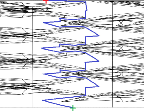
Figure 5: Arrangement of critical curves

We define the critical curves by first assuming that both the segment and the edge at hand (either the robot’s or the obstacle’s) is a full line (containing the edge). We then introduce “critical endpoints” taking into account the fact that the robot’s translation is restricted to a segment and that the edge considered is not a line. This is done by identifying the geometric locus where a vertex and an edge’s endpoint are in contact. We omit this additional stage from the appendix though we addressed it in our work.

0.B.2 Robot representation and definitions

A robot $R$ is a simple polygon with vertices $\{v_{1},\dots,v_{n}\}$ where $v_{i}=(x_{i},y_{i})^{T}$ and edges $\{(v_{1},v_{2}),\dots(v_{n},v_{1})\}$. We assume that the reference point of $R$ is located at the origin. The position of $R$ in the workspace is defined by a configuration $q=(r_{q},\theta_{q})$ where $r_{q}=(x_{q},y_{q})^{T}$.

Thus, $q$ maps the position of a vertex $v_{i}$ by the following parameterization:

$$v_{i}(q)=M(\theta_{q})v_{i}+r_{q},$$

where $M(\theta)=\left[\begin{array}[]{cc}\cos\theta&-\sin\theta\\ \sin\theta&\cos\theta\end{array}\right]$ is the rotation matrix.

Given a segment $seg=[s,t]$ where $s=(x_{s},y_{s})^{T}$ and $t=(x_{t},y_{t})^{T}$ we define the parametrization $(\alpha,\tau)\in[0,1]\times\mathbb{R}$ in Equations (1), (2)

$$r_{q}=(1-\alpha)s+\alpha t,$$ (1)

$$\theta_{q}=2\arctan\tau.$$ (2)

The parametrization fixes the robot’s reference point to the supporting line of $seg$. The parametrized vertex is represented in Equation (3)

$$v_{i}(\alpha,\tau)=M(\tau)v_{i}+(1-\alpha)s+\alpha t,$$ (3)

where $M(\tau)=\frac{1}{1+\tau^{2}}\left[\begin{array}[]{cc}1-\tau^{2}&-2\tau\\ 2\tau&1-\tau^{2}\end{array}\right]$.

0.B.3 Robot’s vertex - Obstacle’s edge

Let $v_{i}$ be a robot’s vertex and $e$ be an obstacle’s edge that is supported by the line $l:ax+by+c=0$. The critical curve in this case is defined by adding the constraint that $v_{i}(q)\in l$ thus:

$$ax_{i}(q)+by_{i}(q)+c=0.$$ (4)

Plugging Equation (3) into Equation (4) yields:
$a[(1-\tau^{2})x_{i}-2\tau y_{i}]+a(1+\tau^{2})(1-\alpha)x_{s}+a(1+\tau^{2})\alpha x_{t}+$
$b[(2\tau)x_{i}+(1-\tau^{2})y_{i}]+b(1+\tau^{2})(1-\alpha)y_{s}+b(1+\tau^{2})\alpha y_{t}+$
$c(1+\tau^{2})=0$,
when simplified:
$\tau^{2}\cdot[-ax_{i}+ax_{s}-by_{i}+by_{s}+c]+$
$\tau\cdot[-2ay_{i}+2bx_{i}]+$ $1\cdot[ax_{i}+ax_{s}+by_{i}+by_{s}+c]+$
$\alpha\tau^{2}\cdot[-ax_{s}+ax_{t}-by_{s}+by_{t}]+$ $\alpha\cdot[-ax_{s}+ax_{t}-by_{s}+by_{t}]=0$.

Hence:

$$\alpha=\frac{p_{2}\tau^{2}+p_{1}\tau+p_{0}}{q_{2}\tau^{2}+q_{0}},$$ (5)

where

$p_{2}=a(x_{i}-x_{s})+b(y_{i}-y_{s})-c$, $p_{1}=2(ay_{i}-bx_{i})$, $p_{0}=-a(x_{i}+x_{s})-b(y_{i}+y_{s})-c$, $q_{2}=a(x_{t}-x_{s})+b(y_{t}-y_{s})$, $q_{0}=q_{2}$.

0.B.4 Robot’s edge - Obstacle’s vertex

Let $e=(v_{1},v_{2})$ be a robot’s edge and $v_{0}$ be an obstacle’s vertex. The critical curve in this case is defined by adding the constraint that $v_{0}$ lies on the line $l:ax+by+c=0$ supporting $e$. To simplify the notation we will consider $\widetilde{l}:(1+\tau^{2})ax+(1+\tau^{2})by+(1+\tau^{2})c=0$ and the constraint that $v_{0}\in\widetilde{l}$. This line has the following coefficients: $(1+\tau^{2})a=(1+\tau^{2})(y_{2}(q)-y_{1}(q))$, $(1+\tau^{2})b=(1+\tau^{2})(x_{1}(q)-x_{2}(q))$ and $(1+\tau^{2})c=(1+\tau^{2})(x_{2}(q)y_{1}(q)-x_{1}(q)y_{2}(q))$. Let us denote $\Delta_{x}=(x_{2}-x_{1})$ and $\Delta_{y}=(y_{2}-y_{1})$.

Simplifying the coefficients of $\widetilde{l}$ yields:

$(1+\tau^{2})a$	=	$(1+\tau^{2})(y_{2}(q)-y_{1}(q))$
	=	$[(2\tau)x_{2}+(1-\tau^{2})y_{2}]+(1+\tau^{2})[(1-\alpha)y_{s}+\alpha y_{t}]$
		$-[(2\tau)x_{1}+(1-\tau^{2})y_{1}]-(1+\tau^{2})[(1-\alpha)y_{s}+\alpha y_{t}]$
	=	$[\Delta_{y}+(2\Delta_{x})\tau-\Delta_{y}\tau^{2}]$,
$(1+\tau^{2})b$	=	$(1+\tau^{2})(x_{1}(q)-x_{2}(q))$
	=	$[(1-\tau^{2})x_{1}-2\tau y_{1}]+(1+\tau^{2})[(1-\alpha)x_{s}+\alpha x_{t}]$
		$-[(1-\tau^{2})x_{2}-2\tau y_{2}]-(1+\tau^{2})[(1-\alpha)x_{s}+\alpha x_{t}]$
	=	$[-\Delta_{x}+\Delta_{y}2\tau+\Delta_{x}\tau^{2}]$,
$(1+\tau^{2})c$	=	$(1+\tau^{2})(x_{2}(q)y_{1}(q)-x_{1}(q)y_{2}(q))$
	=	$(1+\tau^{2})[\frac{1}{1+\tau^{2}}[(1-\tau^{2})x_{2}-2\tau y_{2}]+(1-\alpha)x_{s}+\alpha x_{t}]$
		$[\frac{1}{1+\tau^{2}}[(2\tau)x_{1}+(1-\tau^{2})y_{1}]+(1-\alpha)y_{s}+\alpha y_{t}]$
		$-(1+\tau^{2})[\frac{1}{1+\tau^{2}}[(1-\tau^{2})x_{1}-2\tau y_{1}]+(1-\alpha)x_{s}+\alpha x_{t}]$
		$[\frac{1}{1+\tau^{2}}[(2\tau)x_{2}+(1-\tau^{2})y_{2}]+(1-\alpha)y_{s}+\alpha y_{t}]$
	=	$\frac{1}{(1+\tau^{2})}[-4(x_{1}y_{2}-x_{2}y_{1})\tau^{2}-(x_{1}y_{2}-x_{2}y_{1})(1-\tau^{2})^{2}]$
		$+[(1-\tau^{2})\Delta_{x}-2\tau\Delta_{y}][y_{s}+(y_{t}-y_{s})\alpha]$
		$+[-2\tau\Delta_{x}-(1-\tau^{2})\Delta_{y}][x_{s}+(x_{t}-x_{s})\alpha]$

$(1+\tau^{2})c$	=	$-(1+\tau^{2})(x_{1}y_{2}-x_{2}y_{1})$
		$+(\Delta_{x}-2\Delta_{y}\tau-\Delta_{x}\tau^{2})(y_{s}+(y_{t}-y_{s})\alpha)$
		$+(-\Delta_{y}-2\Delta_{x}\tau+\Delta_{y}\tau^{2})(x_{s}+(x_{t}-x_{s})\alpha)$.

Denoting $k=x_{1}y_{2}-x_{2}y_{1}$ and inserting $v_{0}$ into the line equation of $\widetilde{l}$yields:
$[\Delta_{y}+(2\Delta_{x})\tau-\Delta_{y}\tau^{2}]x_{0}$ $+[-\Delta_{x}+\Delta_{y}2\tau+\Delta_{x}\tau^{2}]y_{0}$ $-k(1+\tau^{2})$
$+[\Delta_{x}-2\Delta_{y}\tau-\Delta_{x}\tau^{2}][y_{s}+(y_{t}-y_{s})\alpha]$ $+[-\Delta_{y}-2\Delta_{x}\tau+\Delta_{y}\tau^{2}][x_{s}+(x_{t}-x_{s})\alpha]=0$.

Now,
$\tau^{2}\cdot[\Delta_{x}(y_{0}-y_{s})-\Delta_{y}(x_{0}-x_{s})-k]+$
$\tau\cdot[2\Delta_{x}(x_{0}-x_{s})+2\Delta_{y}(y_{0}-y_{s})]+$ $1\cdot[-\Delta_{x}(y_{0}-y_{s})+\Delta_{y}(x_{0}-x_{s})-k]+$
$\alpha\tau^{2}\cdot[-\Delta_{x}(y_{t}-y_{s})+\Delta_{y}(x_{t}-x_{s})]+$
$\alpha\tau\cdot[-2\Delta_{y}(y_{t}-y_{s})-2\Delta_{x}(x_{t}-x_{s})]+$ $\alpha\cdot[\Delta_{x}(y_{t}-y_{s})-\Delta_{y}(x_{t}-x_{s})]=0$.

Finally:

$$\alpha=\frac{m_{2}\tau^{2}+m_{1}\tau+m_{0}}{n_{2}\tau^{2}+n_{1}\tau+n_{0}},$$ (6)

where

$m_{2}=\Delta_{y}(x_{0}-x_{s})-\Delta_{x}(y_{0}-y_{s})+k$, $m_{1}=-2\Delta_{x}(x_{0}-x_{s})-2\Delta_{y}(y_{0}-y_{s})$, $m_{0}=-m_{2}+2k$, $n_{2}=\Delta_{y}(x_{t}-x_{s})-\Delta_{x}(y_{t}-y_{s})$, $n_{1}=-2\Delta_{x}(x_{t}-x_{s})-2\Delta_{y}(y_{t}-y_{s})$, $n_{0}=-n_{2}$ and

$\Delta_{x}=(x_{2}-x_{1})$ , $\Delta_{y}=(y_{2}-y_{1})$ , $k=x_{1}y_{2}-x_{2}y_{1}$.

References

- [1] B. Aronov and M. Sharir. On translational motion planning of a convex polyhedron in 3-space. SIAM J. Comput., 26(6):1785–1803, 1997.
- [2] M. H. Austern. Generic Programming and the STL. Addison-Wesley, 1998.
- [3] F. Avnaim, J.-D. Boissonnat, and B. Faverjon. A practical exact motion planning algorithm for polygonal object amidst polygonal obstacles. In Proceedings of the Workshop on Geometry and Robotics, pages 67–86, Springer-Verlag, 1989.
- [4] S. Basu, R. Pollack, and M.-F. Roy. Algorithms in Real Algebraic Geometry. Algorithms and Computation in Mathematics. Springer-Verlag, 2003.
- [5] E. Berberich, E. Fogel, D. Halperin, K. Mehlhorn, and R. Wein. Arrangements on parametric surfaces I: General framework and infrastructure. Mathematics in Computer Science, 4(1):45–66, 2010.
- [6] E. Berberich, M. Hemmer, and M. Kerber. A generic algebraic kernel for non-linear geometric applications. In SoCG 2011.
- [7] J. Canny, B. Donald, and E. K. Ressler. A rational rotation method for robust geometric algorithms. In SoCG 1992, pages 251–260, ACM.
- [8] J. F. Canny. Complexity of Robot Motion Planning (ACM Doctoral Dissertation Award). The MIT Press, June 1988.
- [9] B. Chazelle, H. Edelsbrunner, L. J. Guibas, and M. Sharir. A singly exponential stratification scheme for real semi-algebraic varieties and its applications. Theoretical Computer Science, 84(1):77 – 105, 1991.
- [10] H. Choset, W. Burgard, S. Hutchinson, G. Kantor, L. E. Kavraki, K. Lynch, and S. Thrun. Principles of Robot Motion: Theory, Algorithms, and Implementation. MIT Press, June 2005.
- [11] M. De Berg, O. Cheong, M. van Kreveld, and M. Overmars. Computational Geometry: Algorithms and Applications. Springer, 2008.
- [12] E. Fogel and D. Halperin. Exact and efficient construction of Minkowski sums of convex polyhedra with applications. CAD, 39(11):929–940, 2007.
- [13] P. Hachenberger. Exact Minkowksi sums of polyhedra and exact and efficient decomposition of polyhedra into convex pieces. Algorithmica, 55(2):329–345, 2009.
- [14] D. Halperin and M. Sharir. A near-quadratic algorithm for planning the motion of a polygon in a polygonal environment. Disc. Comput. Geom., 16(2):121–134, 1996.
- [15] S. Hirsch and D. Halperin. Hybrid motion planning: Coordinating two discs moving among polygonal obstacles in the plane. In WAFR 2002, pages 225–241.
- [16] D. Hsu, J. Latombe, and R. Motwani. Path planning in expansive configuration spaces. Int. J. Comp. Geo. & App., 4:495–512, 1999.
- [17] L. E. Kavraki, M. N. Kolountzakis, and J.-C. Latombe. Analysis of probabilistic roadmaps for path planning. IEEE Trans. Robot. Automat., 14(1):166–171, 1998.
- [18] L. E. Kavraki, P. Svestka, J.-C. Latombe, and M. Overmars. Probabilistic roadmaps for path planning in high dimensional configuration spaces. IEEE Transactions on Robotics and Automation, 12(4):566–580, 1996.
- [19] J. J. Kuffner and S. M. Lavalle. RRT-Connect: An efficient approach to single-query path planning. In ICRA 00’, pages 995–1001, 2000.
- [20] A. M. Ladd and L. E. Kavraki. Generalizing the analysis of PRM. In Proceedings of the 2002 IEEE International Conference on Robotics and Automation (ICRA 2002), pages 2120–2125, IEEE Press, 2002.
- [21] J.-C. Latombe. Robot Motion Planning. Kluwer Academic Publishers, Norwell, MA, USA, 1991.
- [22] S. M. Lavalle. Rapidly-exploring random trees: A new tool for path planning. In Computer Science Dept., Iowa State University, Tech. Rep:98–11, 1998.
- [23] S. M. LaValle. Planning Algorithms. Cambridge University Press, Cambridge, U.K., 2006.
- [24] J.-M. Lien. Hybrid motion planning using Minkowski sums. In RSS 2008.
- [25] T. Lozano-Perez. Spatial planning: A configuration space approach. MIT AI Memo 605, 1980.
- [26] N. Mayer, E. Fogel, and D. Halperin. Fast and robust retrieval of Minkowski sums of rotating convex polyhedra in 3-space. In SPM, pages 1–10, 2010.
- [27] E. Plaku, K. E. Bekris, and L. E. Kavraki. OOPS for motion planning: An online open-source programming system. In ICRA, pages 3711–3716, IEEE, 2007.
- [28] J. H. Reif. Complexity of the mover’s problem and generalizations. In FOCS, pages 421–427, IEEE Computer Society, 1979.
- [29] J. T. Schwartz and M. Sharir. On the ”piano movers” problem: I. The case of a two-dimensional rigid polygonal body moving amidst polygonal barriers. Commun. Pure appl. Math, 35:345 – 398, 1983.
- [30] J. T. Schwartz and M. Sharir. On the ”piano movers” problem: II. General techniques for computing topological properties of real algebraic manifolds. Advances in Applied Mathematics, 4(3):298 – 351, 1983.
- [31] M. Sharir. Algorithmic Motion Planning, Handbook of Discrete and Computational Geometry. 2nd Edition, CRC Press, Inc., Boca Raton, FL, USA, 2004.
- [32] J. G. Siek, L.-Q. Lee, and A. Lumsdaine. The Boost Graph Library: User Guide and Reference Manual. Addison-Wesley Professional, 2001.
- [33] The CGAL Project. CGAL User and Reference Manual. CGAL Editorial Board, 3.7 edition, 2010. http //www.cgal.org/.
- [34] R. Wein. Exact and efficient construction of planar Minkowski sums using the convolution method. In ESA, pages 829–840, 2006.
- [35] J. Yang and E. Sacks. RRT path planner with 3 DOF local planner. In ICRA, pages 145–149, 2006.
- [36] L. Zhang, Y. J. Kim, and D. Manocha. A hybrid approach for complete motion planning. In IROS, pages 7–14, 2007.