Theory of optical transitions in graphene nanoribbons

Abstract

Matrix elements of electron-light interactions for armchair and zigzag graphene nanoribbons are constructed analytically using a tight-binding model. The changes in wavenumber ($\Delta n$) and pseudospin are the necessary elements if we are to understand the optical selection rule. It is shown that incident light with a specific polarization and energy, induces an indirect transition ($\Delta n=\pm 1$), which results in a characteristic peak in the absorption spectra. Such a peak provides evidence that the electron standing wave is formed by multiple reflections at both edges of a ribbon. It is also suggested that the absorption of low-energy light is sensitive to the position of the Fermi energy, direction of light polarization, and irregularities in the edge. The effect of depolarization on the absorption peak is briefly discussed.

I Introduction

The dynamics of the electrons in graphene is governed by an equation that is similar to the relativistic equation for the massless Dirac fermion. Novoselov et al. (2005); Zhang et al. (2005) Since the Fermi velocity of a carrier is about $10^{6}$m/s, the Dirac fermion moves forward 1 nm in 1 fs. Therefore, in nanometer-sized graphene, the carrier reaches the edge before its motion is affected by perturbations such as electron-phonon and electron-electron interactions. As a result, the electronic properties of the system are sensitive to the presence of an edge. The behavior of electrons near the edge of a graphene sample is unique due to the reflection of the massless Dirac fermion.

In graphene nanoribbons, the importance of the edge is marked by reflections of electron taking place at the both edges of the ribbon. Li et al. (2008); Jia et al. (2009); Wang and Dai (2010); Berry and Mondragon (1987) The reflections result in the formation of a standing wave of a Dirac fermion. In this paper, we examine optical transitions in graphene nanoribbons and clarify characteristic features of the standing wave of a Dirac fermion. Knowing the rules for the optical transitions is an important step in understanding the optical properties of graphene nanoribbons.

Graphene edges are categorized into two groups: armchair and zigzag edges with respect to the symmetry of the hexagonal lattice. Tanaka et al. (1987); Fujita et al. (1996); Nakada et al. (1996) It is known that standing waves near the armchair edge and near the zigzag edge are distinct for various reasons, such as their pseudospin and Berry’s phase. Sasaki et al. (2010a) In this paper, we study nanoribbons with armchair and zigzag edges in great detail, and briefly discuss the effect of irregularities in the edge on the absorption spectra.

Here, we mention previously published literature on the optical absorption of graphene nanoribbons. Hsu and Reichl Hsu and Reichl (2007) investigated the absorption of linearly polarized light parallel to a zigzag nanoribbon and found that a direct transition is not allowed, in contrast to the case of nanotubes. Ajiki and Ando (1994) Gundra and Shukla Gundra and Shukla (2011) pointed out that the polarization dependence on the absorption spectra is important for characterizing the edge structure. Whereas these studies were based on numerical simulations, our study provides analytical results for electron-light matrix elements. The analytical result clearly shows the effects of pseudospin and momentum conservation on the optical properties of a graphene nanoribbon.

This paper is organized as follows. In Sec. II, we deal with armchair nanoribbons. By constructing the matrix elements of the electron-light interaction, we show that dynamical conductivity depends on the direction of the polarization of the incident light with respect to the orientation of the edge. In Sec. III, we examine absorption spectra for zigzag nanoribbons. The effect of edge irregularities on dynamical conductivity is studied in Sec. IV. Our discussion and conclusion are provided in Secs. V and VI, respectively.

II Armchair nanoribbon

In this section we study the electron-light interaction in armchair nanoribbons. In Sec. II.1, we review the electronic properties of armchair nanoribbons to provide the necessary background. In Sec. II.2, the matrix elements of electron-light interaction are constructed. The results are used to clarify the absorption spectra in Sec. II.3.

II.1 Electron wavefunction

The energy dispersion relation for armchair nanoribbons Compernolle et al. (2003); Zheng et al. (2007); Sasaki et al. (2011) is written as

$$\varepsilon^{s}(k,\theta)=s\gamma_{0}\sqrt{1+4\cos^{2}\theta+4\cos\theta\cos kl},$$ (1)

where $\gamma_{0}$ is the hopping integral ($\gamma_{0}=3$ eV) and $l\equiv\sqrt{3}a/2$ ($a$ is a lattice constant [$a=2.46$ Å]). The energy is characterized by the band index $s$ and two parameters $k$, and $\theta$. The superscript, $s$, represents the conduction (valence) energy band and takes values $s=1$ ($-1$) on the right-hand side of Eq. (1), $k$ is the wave vector parallel to the edge, and $\theta$ stands for the phase in the direction perpendicular to the edge [see Fig. 1(a)]. By setting $k=0$ and $\theta=2\pi/3$ into Eq. (1), we see that $\varepsilon^{s}(0,2\pi/3)=0$ is satisfied. Thus, the conduction and valence energy bands touch at the point $(k,\theta)=(0,2\pi/3)$, which is called the Dirac point. The energy dispersion relation for armchair nanoribbons Eq. (1) is the same as that for graphene. Saito et al. (1998) There are two independent Dirac points (known as K and K^′ points) in the Brillouin zone (BZ) of graphene, on the other hand, there is a single Dirac point in the BZ of armchair nanoribbons. That is, although $\varepsilon^{s}(k,\theta)$ is zero at the other point $(k,\theta)=(0,-2\pi/3)$, this point is not included in the BZ of armchair nanoribbons. In fact, the BZ of armchair nanoribbons is given by $\theta\in(0,\pi)$ and $kb\in[-\pi,\pi)$, where $b\equiv\sqrt{3}a$, as shown in Fig. 1(b). The BZ of armchair nanoribbons covers only one-half of the graphene’s BZ because the reflection taking place at the armchair edge identifies $\theta$ with $-\theta$. Sasaki et al. (2011)

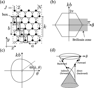
Figure 1: (a) The structure of an $N$ armchair nanoribbon. The unit length along the edge is denoted by $b$ ($\equiv\sqrt{3}a$). Carbon atoms are divided into A ($\bullet$) and B ($\circ$) atoms. (b) The BZ of armchair nanoribbons: $\theta\in(0,\pi)$ and $kb\in[-\pi,\pi)$. The circle stands for the Dirac point. (c) The definition of the polar angle $\Theta(k,\theta)$. The circle represents an energy contour (1 eV). (d) Schematic diagrams for intra- and inter-band transitions from the initial state with $\Theta_{n}=0$ (on the $\theta$-axis).

The wave function is given by

$$\phi^{s}_{J}(k,\theta)=\frac{1}{\sqrt{N}}e^{-ikl(J-1)}\sin J\theta\begin{pmatrix}e^{-i\Theta(k,\theta)}\cr s\end{pmatrix},$$ (2)

where $J$ $(=1,\ldots,N)$ is the coordinate perpendicular to the edge [see Fig. 1(a)]. Compernolle et al. (2003); Zheng et al. (2007); Sasaki et al. (2011) A detailed derivation of the wave function is given in Ref. Sasaki et al., 2011. The upper (lower) component of Eq. (2) represents the amplitude at A-atom (B-atom) in the box shown in Fig. 1(a). The relative phase between the two components, $\Theta(k,\theta)$ in Eq. (2), is the polar angle defined with respect to the Dirac point as shown in Fig. 1(c). The wave function with $\theta=2\pi/3$ does not have an amplitude at $J=3,6,\ldots$ due to $\sin(J\theta)$ of Eq. (2). The corresponding line nodes have been observed in recent scanning tunneling microscopy topography, Yang et al. (2010) which evidences the wave function Eq. (2).

The wave function vanishes at $J=0$ and $J=N+1$ (i.e., at fictitious edge sites). The boundary condition for $J=0$ is given by $\phi^{s}_{J=0}(k,\theta)=0$, which is satisfied with arbitrary values of $\theta$. The phase $\theta$ is quantized by the boundary condition for $J=N+1$, $\phi^{s}_{N+1}(k,\theta)=0$, as

$$\theta_{n}=\frac{n\pi}{N+1},\ \ (n=1,\ldots,N),$$ (3)

where $n$ represents the subband index. Meanwhile, we assume that the wave vector $k$ parallel to the edge is a continuous variable. Because $k$ is not changed by the perturbations, which preserve translational symmetry along the edge, hereafter, we abbreviate $\phi^{s}_{J}(k,\theta_{n})$, $\Theta(k,\theta_{n})$, and $\varepsilon^{s}(k,\theta_{n})$ by omitting $k$ and $\theta$ as $\phi^{s}_{n,J}$, $\Theta_{n}$, and $\varepsilon^{s}_{n}$, respectively.

II.2 Selection rule

The electron-light interaction is written as $H_{\rm em}=-e\mbox{\boldmath$v$}\cdot{\bf A}$, where $-e$ is the electron charge, $\mbox{\boldmath$v$}=(v_{x},v_{y})$ is the velocity operator, and ${\bf A}\propto e^{-i\omega t}\mbox{\boldmath$\epsilon$}$ is a spatially uniform vector potential. Here, $\hbar\omega$ corresponds to the energy of the incident light and $\epsilon$ denotes the polarization. The matrix elements of $v$ are classified into inter-band $\langle\phi_{n}^{c}|\mbox{\boldmath$v$}|\phi_{m}^{v}\rangle$ and intra-band $\langle\phi_{n}^{c}|\mbox{\boldmath$v$}|\phi_{m}^{c}\rangle$ transitions. The contributions of these transitions to the optical property of a nanoribbon depend not only on $\hbar\omega$ and $\epsilon$, but also on the position of the Fermi energy $\varepsilon_{\rm F}$. The intra-band transition may be omitted only when $\varepsilon_{\rm F}=0$ (band center) at zero temperature. In general, it is necessary to consider both transitions.

First, we consider the intra-band transition. The matrix elements of $v$ are calculated using Eq. (2). The details of the calculation are provided in Appendix A. The results are

$$\langle\phi^{c}_{m}|v_{x}|\phi^{c}_{n}\rangle=\begin{cases}\displaystyle 0&\text{$m-n\in$ even}\\ \displaystyle-i\frac{2}{\pi}\frac{v_{\rm F}}{m-n}\langle\sigma_{x}\rangle_{mn}&\text{$m-n\in$ odd},\end{cases}$$ (4)

$$\langle\phi^{c}_{m}|v_{y}|\phi^{c}_{n}\rangle=\delta_{mn}v_{\rm F}\langle\sigma_{y}\rangle_{mn},$$ (5)

where $\delta_{mn}$ is the Kronecker delta, $v_{\rm F}$ ($\equiv\gamma_{0}l/\hbar$) is the Fermi velocity, and $\sigma_{i}$ ($i=x,y$) denotes the Pauli matrices. The matrix elements of $\sigma_{i}$ are written as

$$\langle\sigma_{x}\rangle_{mn}=\frac{1}{2}\left(e^{i\Theta_{m}}+e^{-i\Theta_{n}}\right),$$ (6)

$$\langle\sigma_{y}\rangle_{mn}=-\frac{i}{2}\left(e^{i\Theta_{m}}-e^{-i\Theta_{n}}\right).$$ (7)

$\sigma_{i}$ is the pseudospin, which brings certain features to the optical transitions. For example, in Eq. (6), $\langle\sigma_{x}\rangle_{mn}=1$ is satisfied for forward scattering from $\Theta_{n}=0$ to $\Theta_{m}=0$, while $\langle\sigma_{x}\rangle_{mn}=0$ for backward scattering from $\Theta_{n}=0$ to $\Theta_{m}=\pi$ [see Fig. 1(d)]. Since $\langle\sigma_{x}\rangle_{mn}$ is proportional to $\langle\phi^{c}_{m}|v_{x}|\phi^{c}_{n}\rangle$ as described in Eq. (4), the $x$-polarized light ($A_{x}$) does not cause intra-band backward scattering.

In Eq. (4), the factor in front of the pseudospin $\langle\sigma_{x}\rangle_{mn}$ arises from momentum conservation. It can be shown that momentum conservation for $\langle\phi^{c}_{m}|v_{x}|\phi^{c}_{n}\rangle$ leads to the following summation with respect to the out-of-phase trigonometric functions (Appendix A):

$$\frac{2}{N}\sum_{J=1}^{N}\sin(J\theta_{m})\cos(J\theta_{n})=\begin{cases}\displaystyle 0&\text{$m-n\in$ even}\\ \displaystyle\frac{2}{\pi}\frac{1}{m-n}&\text{$m-n\in$ odd},\end{cases}$$ (8)

where $\theta_{m(n)}$ is given by Eq. (3). The summation takes a non-zero value only when $m-n$ ($\equiv\Delta n$) is an odd number. The momentum conservation for $\langle\phi^{c}_{m}|v_{y}|\phi^{c}_{n}\rangle$ leads to the summation of the in-phase trigonometric functions [see Eq. (38)], so that the summation takes a non-zero value only for $m=n$. Hereafter, we call the process satisfying $m-n\in$ odd an indirect transition for which the wavenumber of the initial state changes ($\Delta n\in$ odd), and the process satisfying $m=n$ is called a direct transition ($\Delta n=0$).

We have seen that the velocity matrix element is determined by two factors: pseudospin and momentum conservation. Next, we consider the inter-band transition based on this understanding. The calculated matrix elements are given by

$$\langle\phi^{c}_{m}|v_{x}|\phi^{v}_{n}\rangle=\begin{cases}\displaystyle 0&\text{$m-n\in$ even}\\ \displaystyle-\frac{2}{\pi}\frac{v_{\rm F}}{m-n}\langle\sigma_{y}\rangle_{mn}&\text{$m-n\in$ odd},\end{cases}$$ (9)

$$\langle\phi^{c}_{m}|v_{y}|\phi^{v}_{n}\rangle=i\delta_{mn}v_{\rm F}\langle\sigma_{x}\rangle_{mn}.$$ (10)

In Eq. (10), $\delta_{mn}$ shows that the $y$-polarized light ($A_{y}$) results in a direct inter-band transition [see Fig. 1(d)]. Thus, the transition amplitude depends on the diagonal matrix element of the pseudospin $\langle\sigma_{x}\rangle_{nn}$. From Eq. (6), we see that $\langle\sigma_{x}\rangle_{nn}$ takes a maximum value of $\langle\sigma_{x}\rangle_{nn}=\cos\Theta_{n}=\pm 1$ for $\Theta_{n}=0$ or $\pi$. On the other hand, $\langle\sigma_{x}\rangle_{nn}$ vanishes for $\Theta_{n}=\pm\pi/2$. Therefore, the electrons on the $\theta$-axis ($\Theta_{n}=0$ or $\pi$) are selectively excited by $A_{y}$, while the electrons near the $k$-axis ($\Theta_{n}=\pm\pi/2$) are excited very little.

As we can see in Eq. (9), the $x$-polarized light ($A_{x}$) results in an indirect transition [see Fig. 1(d)]. An inter-band transition amplitude from $\Theta_{n}=0$ to $\Theta_{m}=\pi$ is enhanced because the strength of the pseudospin takes a maximum value of $|\langle\sigma_{y}\rangle_{mn}|=1$. This indirect inter-band transition is a forward scattering, namely, the electron crosses the Dirac point. An inter-band transition that is not across the Dirac point, such as a (backward) transition from $\Theta_{n}=0$ to $\Theta_{m}=0$, is allowed by momentum conservation if $m-n$ is an odd number. However, it is strongly suppressed by the pseudospin because $\langle\sigma_{y}\rangle_{mn}=0$ for the process.

II.3 Dynamical conductivity

With the optical selection rule established by Eqs. (4), (5), (9), and (10), let us investigate the absorption of light. The dynamical conductivity is given by ($\alpha=x,y$)

$$\sigma_{\alpha\alpha}(\omega)=\frac{\hbar}{iS}\sum_{s^{\prime}s}\sum_{nmk}\frac{\left(f[\varepsilon^{s^{\prime}}_{m}]-f[\varepsilon^{s}_{n}]\right)\left|\langle\phi^{s^{\prime}}_{m}|(-ev_{\alpha})|\phi^{s}_{n}\rangle\right|^{2}}{\left(\varepsilon^{s^{\prime}}_{m}-\varepsilon^{s}_{n}\right)\left(\varepsilon^{s^{\prime}}_{m}-\varepsilon^{s}_{n}+\hbar\omega+i\delta\right)},$$ (11)

where $f[\varepsilon]$ is the Fermi distribution function, $S$ is the nanoribbon area, and $\delta$ is inversely proportional to the relaxation time of the excited electron. Ando et al. (2002) The real part of the dynamical conductivity, ${\rm Re}(\sigma_{xx})$ (${\rm Re}(\sigma_{yy})$), represents the absorption spectrum of $x$-polarized ($y$-polarized) light. In Eq. (11), we assume $\delta=10$ meV and room temperature when evaluating the Fermi distribution function.

The solid curve in Fig. 2(a) shows ${\rm Re}(\sigma_{yy})$ calculated for an $N=15$ armchair nanoribbon. The width of this nanoribbon is 1.7 nm. As we have shown in Eq. (10), the absorption of $y$-polarized light results from a direct inter-band transition. Thus, the peaks denoted by A, B, and C of ${\rm Re}(\sigma_{yy})$ originate from the direct inter-band transitions $\phi^{v}_{n}\to\phi^{c}_{n}$ (A), $\phi^{v}_{n-1}\to\phi^{c}_{n-1}$ (B), and $\phi^{v}_{n+1}\to\phi^{c}_{n+1}$ (C), respectively, as shown in Fig. 2(b). The energy position of the A peak corresponds to the energy gap ($E_{\rm gap}$) of 0.66 eV for an $N=15$ armchair nanoribbon. Both a large density of states at the band edge ($k=0$) of each subband and the pseudospin are important as regards enhancing these peak intensities.

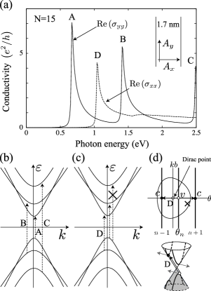
Figure 2: (a) The calculated ${\rm Re}(\sigma_{\alpha\alpha})$ for an $N=15$ (semiconducting) armchair nanoribbon. The inter-band transition processes relevant to the absorption peaks of ${\rm Re}(\sigma_{yy})$ and ${\rm Re}(\sigma_{xx})$ are shown in (b) and (c), respectively. (d) The optically allowed indirect inter-band transition (from $\phi_{n}^{v}$ to $\phi_{n-1}^{c}$ or from $\phi_{n-1}^{v}$ to $\phi_{n}^{c}$). Bottom: The pseudospin (denoted by arrows) is useful for showing that only forward scattering is allowed in the inter-band optical transitions.

The dashed curve in Fig. 2(a) represents ${\rm Re}(\sigma_{xx})$. As we have seen in Eq. (9), the absorption of $x$-polarized light is the result of an indirect inter-band transition. Thus, the peak denoted by D of ${\rm Re}(\sigma_{xx})$ is due to the transitions $\phi^{v}_{n}\to\phi^{c}_{n-1}$ and $\phi^{v}_{n-1}\to\phi^{c}_{n}$, as shown in Fig. 2(c). Because the resonance energy ($\varepsilon^{c}_{n}-\varepsilon^{v}_{n-1}$) is between $\varepsilon^{c}_{n}-\varepsilon^{v}_{n}$ and $\varepsilon^{c}_{n-1}-\varepsilon^{v}_{n-1}$, which are the resonance energies for the direct inter-band transitions A and B, the peak D appears between the A and B peaks. Note that another indirect transition $\phi^{v}_{n}\to\phi^{c}_{n+1}$ is also allowed by momentum conservation. However, the pseudospin strongly suppresses the backward transition for the states at the band edge ($k=0$) and the large density of states does not result in an absorption peak. Hence, there is no prominent peak for ${\rm Re}(\sigma_{xx})$ between the B and C peaks. Moreover, the peak corresponding to the lowest-energy backward transition is the most prominent, and the peak for the second lowest (and higher) energy transition, such as $\phi^{v}_{n}\to\phi^{c}_{n-3}$ and $\phi^{v}_{n+1}\to\phi^{c}_{n-2}$, is generally suppressed by the momentum conservation giving rise to the suppression factor of $(m-n)^{-1}$ in Eq. (9). To clarify this point, we show the calculated ${\rm Re}(\sigma_{xx})$ for an $N=55$ armchair nanoribbon with $E_{\rm gap}=0.2$ eV in Fig. 3(a). For ${\rm Re}(\sigma_{xx})$, there is only a peak on the low-energy side.

Figure 3: ${\rm Re}(\sigma_{\alpha\alpha})$ of an $N=55$ armchair nanoribbon with an energy gap about 0.2 eV, calculated for (a) $\varepsilon_{\rm F}=0$ eV and (b) $\varepsilon_{\rm F}=0.3$ eV.

It is clear that the absorption spectrum of an armchair nanoribbon exhibits strong anisotropy for the polarization direction of incident light. Gundra and Shukla (2011) More specifically, a number of peaks appear when the polarization is parallel to the armchair nanoribbon, while only a single prominent peak appears on the low-energy side when the polarization is set perpendicular to the ribbon. Because the energy gap of (semiconducting) armchair nanoribbons behaves as $E_{\rm gap}\propto N^{-1}$, Son et al. (2006); White et al. (2007) the energy position of the peak for perpendicular polarization is inversely proportional to the width of the armchair nanoribbon.

Since $\varepsilon_{\rm F}$ is generally not zero, it is meaningful to point out that the absorption of low-energy photons is sensitive to the position of $\varepsilon_{\rm F}$. To explain this feature, we show the dynamical conductivity for an $N=55$ armchair nanoribbon with $\varepsilon_{\rm F}=0.3$ eV in Fig. 3(b). For $E_{\rm gap}<\hbar\omega<2|\varepsilon_{\rm F}|$, ${\rm Re}(\sigma_{yy})$ is suppressed by the Pauli exclusion principle, while a peak remains for ${\rm Re}(\sigma_{xx})$. This peak is attributed to forward intra-band scattering. In addition, the Drude peak at $\hbar\omega=0$ appears only for $y$-polarized light. This feature arises from the fact that the diagonal matrix element of $v_{y}$ can take a non-zero value, while that of $v_{x}$ is zero, as we have seen in Eqs. (4) and (5).

III Zigzag nanoribbon

In this section, we focus on zigzag nanoribbons. We show that the optical properties of zigzag nanoribbons are quantitatively different from those of armchair nanoribbons. For example, when the polarization of an incident light is parallel to the zigzag nanoribbons, the allowed inter-band transitions are indirect transitions. On the other hand, when the light polarization is perpendicular to the ribbons, a direct inter-band transition is allowed. The behavior of zigzag nanoribbons contrasts with that of armchair nanoribbons.

III.1 Electron wavefunction

The energy dispersion relation for zigzag nanoribbons is given by

$$\varepsilon^{s}(k,\theta)=s\gamma_{0}\sqrt{1+4\cos^{2}\left(\frac{ka}{2}\right)+4\cos\left(\frac{ka}{2}\right)\cos\theta},$$ (12)

where $k$ is the wave vector along the zigzag edge, and $\theta$ denotes the phase in the direction perpendicular to the edge [see Fig. 4(a)]. By putting $(k,\theta)=(4\pi/3a,0)$ and $(2\pi/3a,\pi)$ into Eq. (12), we have $\varepsilon^{s}(k,\theta)=0$. The two Dirac points are non-equivalent, i.e., the BZ of zigzag nanoribbons contains the two independent Dirac points (K and K^′) [see Fig. 4(b)]. This contrasts with the fact that the BZ of armchair nanoribbons has a single Dirac point. The difference in the number of Dirac points is because the reflection of an electronic wave at the zigzag edge constitutes intravalley scattering, while the reflection at the armchair edge is intervalley scattering.

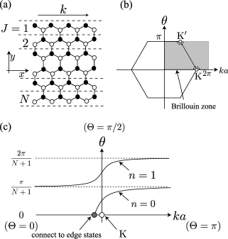
Figure 4: (a) The structure of an $N$ zigzag nanoribbon. (b) The BZ of a zigzag nanoribbon: $\theta\in(0,\pi)$ and $ka\in[0,2\pi)$. The empty circles show the positions of the K and K^′ points. The dashed semicircles around the K and K^′ points represent an energy contour (1 eV). (c) The plot of $\theta_{n}(k)$ for an $N$ zigzag nanoribbon.

The wave function is expressed by

$$\varphi^{s}_{J}(k,\theta)=\frac{1}{2\sqrt{N}}\left\{e^{iJ\theta}\begin{pmatrix}e^{-i\Theta(k,\theta)}\cr s\end{pmatrix}-e^{-iJ\theta}\begin{pmatrix}e^{i\Theta(k,\theta)}\cr s\end{pmatrix}\right\},$$ (13)

where $J$ ($=1,\ldots,N$) is a coordinate perpendicular to the zigzag edge [see Fig. 4(a)]. A detailed derivation of the wave function including the pseudospin is given in Ref. Sasaki et al., 2009. The wave function Eq. (13) is a standing wave formed by the superposition of two waves propagating in opposite directions. The first term on the right-hand side of Eq. (13) represents an incident wave, and the second term corresponds to an edge reflected wave. The phase $\Theta(k,\theta)$ is defined through $|\varepsilon^{s}(k,\theta)|e^{-i\Theta(k,\theta)}=2\cos\left(ka/2\right)+e^{-i\theta}$, Sasaki et al. (2009) by which we can see that $\Theta(k,\theta)$ corresponds to the polar angle defined with respect to the K or K^′ point. For the K point, $\Theta(k,\theta)$ is given as shown in Fig. 4(c). Note that the signs in front of $\Theta(k,\theta)$ for the constituent waves are opposite. This feature can be understood in terms of the reflection of pseudospin, namely, the zigzag edge alters the direction of the pseudospin of an incident wave. Sasaki et al. (2010b) By contrast, the armchair edge does not change the direction of the pseudospin. In fact, in this case, we can reproduce the wave function for armchair edge Eq. (2) as

$$e^{iJ\theta}\begin{pmatrix}e^{-i\Theta}\cr s\end{pmatrix}-e^{-iJ\theta}\begin{pmatrix}e^{-i\Theta}\cr s\end{pmatrix}\propto\sin(J\theta)\begin{pmatrix}e^{-i\Theta}\cr s\end{pmatrix}.$$ (14)

It is the characteristic feature of the zigzag edge that the reflection of the momentum of the incident wave $(\theta\to-\theta)$ accompanies the change of the pseudospin $(\Theta\to-\Theta)$. This correlation between momentum and pseudospin does not exist for armchair nanoribbons.

The wave function has two components

$$\varphi^{s}_{J}=\begin{pmatrix}\varphi^{s}_{{\rm A},J}\cr\varphi^{s}_{{\rm B},J}\end{pmatrix}=\frac{i}{\sqrt{N}}\begin{pmatrix}\sin(J\theta-\Theta(k,\theta))\cr s\sin(J\theta)\end{pmatrix},$$ (15)

where the first (second) component represents the amplitude at A-atom (B-atom) [see Fig. 4(a)]. Note that the minus sign in front of the second term on the right-hand side of Eq. (13) ensures that the wave function satisfies the boundary condition at $J=0$ given by $\varphi^{s}_{{\rm B},J=0}=0$. The phase $\theta$ is quantized as $\theta_{n}$ by the boundary condition at $J=N+1$, $\varphi^{s}_{{\rm A},J=N+1}=0$. This boundary condition gives the constraint condition between $k$ and $\theta_{n}$, $\Theta(k,\theta_{n})-(N+1)\theta_{n}=-n\pi$, which is rewritten as

$$\theta_{n}=\frac{n\pi+\Theta(k,\theta_{n})}{N+1}.$$ (16)

We plot $\theta_{n}$ with $n=0,1$ as a function of $k$ in Fig. 4(c), where $\theta_{n}$ is a curved rather than a straight line. Sasaki et al. (2010a) This feature also contrasts with that of an armchair nanoribbon, for which the quantized $\theta_{n}$ is independent of $k$ [see Eq. (3)]. Note that the curved line of $\theta_{n}(k)$ with $n=0$ reaches the $k$-axis near the Dirac point. It can be shown that $\theta_{0}(k)$ acquires an imaginary part after crossing the $k$-axis as $\theta_{0}(k)=i/\xi(k)$. In Eq. (13), $\xi(k)$ corresponds to the localization length. By putting $\theta_{0}(k)=i/\xi(k)$ into Eq. (16), we see that $\Theta_{0}(k,\theta_{0}(k))$ also acquires an imaginary part as $\Theta_{0}(k,\theta_{0}(k))=i(N+1)/\xi(k)$. This means that the pseudospin is polarized by the localization. The localized states near the zigzag edge are known as the edge states. Tanaka et al. (1987); Fujita et al. (1996) The curved line is essential to the existence of the edge localized states in the zigzag nanoribbons.

III.2 Selection rule

We start by showing the velocity matrix elements with respect to the inter-band transition (see Appendix B for derivation),

$$\begin{split}&\langle\varphi^{c}_{m}|v_{x}|\varphi^{v}_{n}\rangle=iv_{\rm F}\langle\varphi^{c}_{m}|\sigma_{y}|\varphi^{c}_{n}\rangle,\\ &\langle\varphi^{c}_{m}|v_{y}|\varphi^{v}_{n}\rangle=iv_{\rm F}\langle\varphi^{c}_{m}|\sigma_{x}|\varphi^{c}_{n}\rangle.\end{split}$$ (17)

The calculation for the pseudospin of the standing wave, on the right-hand side of Eq. (17), is straightforward with the use of Eqs. (13) and (16). The results are

$$\langle\varphi^{c}_{m}|\sigma_{x}|\varphi^{c}_{n}\rangle= -\sin\Theta_{m}\left\{\frac{\sin^{2}\left[\frac{(n+m)\pi+(\Theta_{n}+\Theta_{m})}{2}\right]}{(n+m)\pi+(\Theta_{n}+\Theta_{m})}+\frac{\sin^{2}\left[\frac{(n-m)\pi+(\Theta_{n}-\Theta_{m})}{2}\right]}{(n-m)\pi+(\Theta_{n}-\Theta_{m})}\right\}$$

$$-\frac{\cos\Theta_{m}}{2}\left\{\frac{\sin\left[(n+m)\pi+(\Theta_{n}+\Theta_{m})\right]}{(n+m)\pi+(\Theta_{n}+\Theta_{m})}-\frac{\sin\left[(n-m)\pi+(\Theta_{n}-\Theta_{m})\right]}{(n-m)\pi+(\Theta_{n}-\Theta_{m})}\right\}+(n\leftrightarrow m),$$ (18)

$$i\langle\varphi^{c}_{m}|\sigma_{y}|\varphi^{c}_{n}\rangle= -\sin\Theta_{m}\left\{\frac{\sin^{2}\left[\frac{(n+m)\pi+(\Theta_{n}+\Theta_{m})}{2}\right]}{(n+m)\pi+(\Theta_{n}+\Theta_{m})}+\frac{\sin^{2}\left[\frac{(n-m)\pi+(\Theta_{n}-\Theta_{m})}{2}\right]}{(n-m)\pi+(\Theta_{n}-\Theta_{m})}\right\}$$

$$-\frac{\cos\Theta_{m}}{2}\left\{\frac{\sin\left[(n+m)\pi+(\Theta_{n}+\Theta_{m})\right]}{(n+m)\pi+(\Theta_{n}+\Theta_{m})}-\frac{\sin\left[(n-m)\pi+(\Theta_{n}-\Theta_{m})\right]}{(n-m)\pi+(\Theta_{n}-\Theta_{m})}\right\}-(n\leftrightarrow m).$$ (19)

First, we consider a case where the polarization of the incident light is parallel to the zigzag nanoribbon. By setting $m=n$ in Eq. (19), we have $\langle\varphi^{c}_{n}|\sigma_{y}|\varphi^{c}_{n}\rangle=0$. Since $\langle\varphi^{c}_{n}|\sigma_{y}|\varphi^{c}_{n}\rangle=0$ leads to $\langle\varphi^{c}_{n}|v_{x}|\varphi^{v}_{n}\rangle=0$ in Eq. (17), we conclude that the $x$-polarized light does not cause a direct inter-band transition. Therefore, the possible inter-band transition is an indirect one. To further explore the inter-band transitions produced by the $x$-polarized light, let us examine the electrons with $\Theta=\pi/2$ (or $k=4\pi/3a$). By putting $\Theta_{n}=\pi/2$ and $\Theta_{m}=\pi/2$ into Eq. (19), we obtain

$$\langle\varphi^{c}_{m}|v_{x}|\varphi^{v}_{n}\rangle=v_{\rm F}\frac{2}{\pi}\frac{\sin^{2}\left(\frac{\pi}{2}\Delta n\right)}{\Delta n}.$$ (20)

Equation (20) suggests that the $x$-polarized light induces indirect transitions when $m-n$ $(\equiv\Delta n)$ is an odd number. The inter-band transitions with $\Delta n=\pm 1$ have advantage over the transitions with $\Delta n=\pm 3,5,\ldots$ in producing prominent peaks in the dynamical conductivity since the suppression due to the momentum conservation is minimum when $\Delta n=\pm 1$.

Next, we consider a case where the polarization of the incident light is perpendicular to the zigzag nanoribbon. When $m=n$, Eq. (18) leads to

$$\langle\varphi^{c}_{n}|\sigma_{x}|\varphi^{c}_{n}\rangle=\cos\Theta_{n}-\frac{\sin\Theta_{n}}{n\pi+\Theta_{n}}.$$ (21)

The second term on the right-hand side is suppressed by the factor of $(\pi n)^{-1}$ when $n\geq 1$. For $n=0$, $\langle\varphi^{c}_{n}|\sigma_{x}|\varphi^{c}_{n}\rangle$ is zero when $\Theta_{0}=0$ and $-1$ when $\Theta_{0}=\pi$. Thus, the $y$-polarized light gives rise to direct inter-band transitions, by which the electrons near the $k$-axis ($\Theta=0$ or $\pi$) are selectively excited. Since there is not a large density of states for the states near the $k$-axis, the direct inter-band transition does not result in a prominent absorption peak.

By putting $\Theta_{n}=\pi/2$ and $\Theta_{m}=\pi/2$ into Eq. (18), we obtain

$$\langle\varphi^{c}_{m}|v_{y}|\varphi^{v}_{n}\rangle=-iv_{\rm F}\frac{2}{\pi}\frac{\sin^{2}\left[\frac{\pi}{2}(n+m+1)\right]}{(n+m+1)}$$ (22)

Equation (22) suggests that the $y$-polarized light gives rise to an indirect inter-band transition when $n+m$ is an even number. For example, the transition $\varphi^{v}_{0}\to\varphi^{c}_{2}$ [which corresponds to the peak C in Fig. 5(c)] satisfies this condition. However, the amplitude of this process is small due to the suppression by momentum conservation. The indirect inter-band transitions caused by $y$-polarized light can be neglected.

Figure 5: (a) Calculated ${\rm Re}(\sigma_{\alpha\alpha})$ for an $N=11$ zigzag nanoribbon. The optical transition processes relevant to (b) ${\rm Re}(\sigma_{xx})$ and (c) ${\rm Re}(\sigma_{yy})$. The flat band at the band center represents the energy dispersion of the edge states.

We have shown that the $x$-polarized light (parallel to the zigzag edge) results in indirect inter-band transitions ($\Delta n=\pm 1$) for the states near the band edges. Hsu and Reichl (2007) The $y$-polarized light induces direct inter-band transitions ($\Delta n=0$) selectively for the states near the $k$-axis. The polarization dependence of the inter-band optical transition in zigzag nanoribbons exhibits a 90^∘ phase shift with respect to that derived for armchair nanoribbons.

The velocity matrix elements for the intra-band transition are written as

$$\begin{split}&\langle\varphi^{c}_{m}|v_{x}|\varphi^{c}_{n}\rangle=-v_{\rm F}\langle\varphi^{c}_{m}|\sigma_{x}|\varphi^{c}_{n}\rangle,\\ &\langle\varphi^{c}_{m}|v_{y}|\varphi^{c}_{n}\rangle=v_{\rm F}\langle\varphi^{c}_{m}|\sigma_{y}|\varphi^{c}_{n}\rangle.\end{split}$$ (23)

From Eqs. (23) and (17), we see that

$$\begin{split}&|\langle\varphi^{c}_{m}|v_{x}|\varphi^{v}_{n}\rangle|=|\langle\varphi^{c}_{m}|v_{y}|\varphi^{c}_{n}\rangle|,\\ &|\langle\varphi^{c}_{m}|v_{y}|\varphi^{v}_{n}\rangle|=|\langle\varphi^{c}_{m}|v_{x}|\varphi^{c}_{n}\rangle|.\end{split}$$ (24)

The equations mean that the selection rule for intra-band transitions can be obtained from that for inter-band transitions by changing the polarization direction. For the intra-band transitions, the $x$-polarized light results in a direct transition ($\Delta n=0$), while the $y$-polarized light results in an indirect transition ($\Delta n=\pm 1$).

III.3 Dynamical conductivity

In Fig. 5(a), we show the calculated ${\rm Re}(\sigma_{\alpha\alpha})$ for an $N=11$ zigzag nanoribbon. The width of the ribbon is 2.2 nm. The solid curve represents ${\rm Re}(\sigma_{xx})$, where the A and B peaks are attributed to the transitions shown in Fig. 5(b). The change in the wavenumber, which is relevant to the A peak, is $\Delta n=\pm 1$, while that relevant to the B peak is $\Delta n=\pm 3$. The intensity of the B peak is much smaller than that of the A peak due to suppression by momentum conservation. The dashed curve represents ${\rm Re}(\sigma_{yy})$, where the small C peak is due to the transitions shown in Fig. 5(c). The finite conductivity at low energy below the C peak originates from the direct transition shown in Fig. 5(c). The conductivity is suppressed near $\hbar\omega=0$. This feature can be explained by the pseudospin of the edge states. Later we discuss the fact that the velocity matrix element between two edge states vanishes because the edge states are pseudospin polarized states (i.e., eigen state of $\sigma_{z}$), so that $\langle\sigma_{x}\rangle_{nn}=0$.

Figure 6: The calculated ${\rm Re}(\sigma_{\alpha\alpha})$ of an $N=50$ zigzag nanoribbon for different Fermi energies: (a) $\varepsilon_{\rm F}=0$ eV and (b) $\varepsilon_{\rm F}=0.3$ eV.

Note that the indirect inter-band transitions A, B, and C in Fig. 5(b) and (c), involve the states near the Dirac point. Hence, we can expect the dynamical conductivity to be sensitive to the position of $\varepsilon_{\rm F}$. To elucidate this point, we show the calculated ${\rm Re}(\sigma_{\alpha\alpha})$ for an $N=50$ zigzag nanoribbon with different $\varepsilon_{\rm F}$ in Fig. 6(a) [$\varepsilon_{\rm F}=0$ eV] and (b) [$\varepsilon_{\rm F}=0.3$ eV]. In Fig. 6(a), the most prominent peak appears for ${\rm Re}(\sigma_{xx})$, which corresponds to the transition A ($\varphi^{v}_{0}\to\varphi^{c}_{1}$) shown in Fig. 5(b). The other peaks are due to $\varphi^{v}_{n}\to\varphi^{c}_{n+1}$ with $n=1,2,\ldots$. By contrast, at a low energy in Fig. 6(b), the peak intensity is suppressed for ${\rm Re}(\sigma_{xx})$ and the most prominent peak appears for ${\rm Re}(\sigma_{yy})$. This change of the polarization dependence is because intra-band transitions, such as D shown in Fig. 5(c), are activated by $y$-polarized light. Finally, the Drude peak appears only when the polarization is set parallel to the zigzag nanoribbon, because the $x$-polarized light provides a direct intra-band transition. This polarization dependence of the Drude peak is analogous to the case of armchair nanoribbon.

IV Irregular edge

In this section, we study the effect of edge irregularities on the dynamical conductivity by employing a numerical simulation based on a tight-binding model. Although the variety of irregular edge structures that we consider is quite limited, the results help us to understand the way in which the absorption spectra are changed by irregularities.

Figure 7(a) displays the calculated ${\rm Re}(\sigma_{\alpha\alpha})$ for a defective $N=15$ armchair nanoribbon (thick lines). We introduced irregularities consisting of zigzag edges along the armchair edge of the ribbon. One of the zigzag parts is shown in the right-hand side of Fig. 7(a). The size of the zigzag part is about $\Delta x=5$ Å and $\Delta y=2$ nm. For comparison, we show ${\rm Re}(\sigma_{\alpha\alpha})$ for a pure armchair nanoribbon without any irregularities (thin lines) in Fig. 7(a). These results show that the irregularities do not induce any significant change in the ${\rm Re}(\sigma_{xx})$ of the regular armchair nanoribbon. A notable effect of the irregularities appears for ${\rm Re}(\sigma_{yy})$ as the new peak at 0.4 eV, denoted by Z. Since the original pure armchair nanoribbon has an energy gap of 0.66 eV, the Z peak originates from irregularities consisting of the zigzag parts. Note that the appearance of the Z peak accompanies a reduction in the peak intensity at 0.66 eV.

Figure 7: The calculated ${\rm Re}(\sigma_{\alpha\alpha})$ in the presence (thick lines) or absence (thin lines) of irregularities for (a) $N=15$ armchair and (c) $N=11$ zigzag nanoribbons. (b) compares ${\rm Re}(\sigma_{\alpha\alpha})$ in the presence of an irregularity consisting of two sublattices (thin lines) with that consisting of one sublattice (thick lines). In the simulation, we assume that the length of the nanoribbon is 40 nm, $\delta=50$ meV, and $\varepsilon_{\rm F}=0$ eV.

Because a small segment of the zigzag edge about 1 nm in length creates a zero-energy edge state in the energy spectrum, Nakada et al. (1996) it is reasonable to consider that the Z peak is relevant to the edge state caused by the irregularity. Moreover, the reduction in the peak intensity at 0.66 eV suggests that the optical transition from the edge state to the state at the band edge of the first subband is activated. This consideration is consistent with the fact that the Z peak position (0.4 eV) is approximately half of the energy band gap of the pure armchair nanoribbon (0.66/2 eV).

An interesting point here is that the edge state existing near the zigzag irregularity can contribute to the optical transition, on the other hand, the edge state in pure zigzag nanoribbons does not. That is, the edge state near a zigzag irregularity is not identical to the edge state in a pure zigzag nanoribbon. For a pure zigzag nanoribbon, the edge atoms at $J=0$ are all A-atoms, while those at $J=N$ are all B-atoms [see Fig. 4(a)]. As a result, the wave function of the edge state localized at $J=0$ is written as

$$\varphi_{\rm A}\propto e^{-\frac{J}{\xi}}\begin{pmatrix}1\cr 0\end{pmatrix},$$ (25)

while the wave function of the edge state localized at $J=N$ is written as

$$\varphi_{\rm B}\propto e^{-\frac{N-J}{\xi}}\begin{pmatrix}0\cr 1\end{pmatrix},$$ (26)

where $\xi$ is the localization length. Note that these edge states have an amplitude only on the A-atoms or B-atoms depending on the edge atom. Since the electron-light matrix element is proportional to the matrix element of $\sigma_{x}$ or $\sigma_{y}$, the matrix elements with respect to the pseudospin polarized edge states vanish as

$$\begin{pmatrix}1&0\end{pmatrix}\sigma_{i}\begin{pmatrix}1\cr 0\end{pmatrix}=0\ \ (i=x,y).$$ (27)

One might consider that the matrix element of $\sigma_{i}$ between the edge state localized at $J=0$ and that localized at $J=N$ can be non-zero because

$$\begin{pmatrix}0&1\end{pmatrix}\sigma_{i}\begin{pmatrix}1\cr 0\end{pmatrix}\neq 0.$$ (28)

However, such matrix elements are also strongly suppressed because $\xi<N$ is satisfied and there is little spatial overlap between the two edge states. Therefore, the edge state in a pure zigzag nanoribbon does not contribute to the optical transition.

By contrast, the edge atoms of the zigzag irregularity include equal numbers of A-atoms and B-atoms, and the A- and B-edge atoms are close in space. Thus, the edge state at the A-edge atoms [$\varphi_{\rm A}({\bf r})$] can interfere with the other edge state at the B-atoms [$\varphi_{\rm B}({\bf r})$] to form a new edge state pair [$\varphi^{c,v}({\bf r})=\varphi_{\rm A}({\bf r})\pm\varphi_{\rm B}({\bf r})$]. This feature of the interference between two sublattices is essential to the optical transition. This consideration is consistent with the result shown in Fig. 7(b), where the intensity of the Z peak decreases when the zigzag edge part consists only of one sublattice. Klein (1994) Note also that the inter-band transition $\varphi^{v}({\bf r})\to\varphi^{c}({\bf r})$ for the edge states contributes to the absorption spectrum at zero-energy ($\hbar\omega\approx 0$) as shown in Fig. 7(a).

In Fig. 7(c), we show ${\rm Re}(\sigma_{\alpha\alpha})$ for a defective $N=11$ zigzag nanoribbon (thick lines) and that for a pure one (thin lines). The irregularities consist of armchair edges. One of the armchair parts is shown in the right-hand side of Fig. 7(c). The irregularities do not result in a notable change of the absorption spectrum. This feature can be rationalized by using the fact that the armchair edge does not change the pseudospin via the reflection of the incident electron wave [see Eq. (14)].

The numerical results presented in this section suggest that for a defective armchair nanoribbon, the absorption spectrum of transversely ($x$) polarized light is robust against the presence of irregularities, while the absorption spectrum of low-energy longitudinally ($y$) polarized light is sensitive to them. For a defective zigzag nanoribbon, the absorption spectrum appears insensitive to the irregularities.

V Discussion

The optical selection rule of armchair nanoribbons reminds us of the optical selection rule of single-wall carbon nanotubes (SWNTs). Ajiki and Ando (1994) The selection rule of SWNTs shows that light polarized parallel (perpendicular) to the axis results in a direct (indirect) inter-band transition satisfying $\Delta n=0$ ($\Delta n=\pm 1$). It is known that the indirect transition originates from the cylindrical topology of SWNTs. Although the indirect transition is interesting, the corresponding absorption peak is suppressed by the depolarization effect. Ajiki and Ando (1994) Indeed, the experimental results for SWNTs do not show absorption peaks relevant to the indirect inter-band transition. This is consistent with the presence of a depolarization field. Hwang et al. (2000); Ichida et al. (2001, 2004) While the topology of nanoribbons is quite different from that of SWNTs, there is a possibility that a depolarization field suppresses the absorption of the $x$-polarized light for armchair nanoribbons. The selection rule for zigzag nanoribbons is distinct from that for armchair nanoribbons, and the zigzag nanoribbons seem to be anomalous with respect to the depolarization effect. The depolarization field points along the $y$-axis, which is orthogonal to the direction of the polarization of the incident light.

The optical transition between two subbands $n$ and $m$ depends on changes in the wavenumber $\Delta n$ ($=m-n$) and the pseudospin $\langle\sigma_{i}\rangle_{mn}$. These factors $\Delta n$ and $\langle\sigma_{i}\rangle_{mn}$ could be treated independently in a discussion of the optical transitions for armchair nanoribbons. On the other hand, the factors mix and cannot be treated independently for zigzag nanoribbons. The pseudospin can be changed by interactions that are not included in our analysis. For example, a potential difference between the A and B sublattices is induced by the stack in the Bernal configuration and gives rise to a polarization of pseudospin for the states near the Dirac point. Sasaki et al. (2011) Furthermore, the pseudospin can be related to real spin because the edge states in zigzag nanoribbons are prone to be spin polarized if we take into account the Coulomb interaction. Fujita et al. (1996); Son et al. (2006) Although the selection rules that we have obtained provide the basis for exploring the optical phenomena exhibited by graphene nanoribbons, it is possible that these interactions modify the absorption peaks present in this paper. Gundra and Shukla (2011)

VI conclusion

We have paid considerable attention to the indirect optical transitions satisfying $\Delta n=\pm 1$. An inter-band transition with $\Delta n=\pm 1$ is induced when the polarization of the incident light is perpendicular (parallel) to the armchair (zigzag) edge, while an intra-band indirect transition is induced when the light polarization is perpendicular to both the armchair and zigzag edges. The indirect optical transitions can be traced to the inter-edge electronic coherence. The signal of the indirect transition appears as a low-energy peak in absorption spectra. The corresponding absorption peak remains in the presence of the irregularity and with different Fermi energy positions, while it may be suppressed by a depolarization field.

Appendix A Derivations of Eqs. (4), (5), (9), and (10)

In this appendix, we give the derivations of the matrix elements of the velocity operator $v$ for armchair nanoribbons. The operator $v$ is defined as the first derivative of the nearest-neighbor tight-binding Hamiltonian, $H({\bf A})$, with respect to a vector potential, ${\bf A}$, as $-e\mbox{\boldmath$v$}=\partial H({\bf A})/\partial{\bf A}|_{{\bf A}=0}$. The electron-light interaction is given by $H_{\rm em}=-e\mbox{\boldmath$v$}\cdot{\bf A}$, and the matrix elements are written as

$$\langle\phi^{c}_{m}|\left(-e\mbox{\boldmath$v$}\cdot{\bf A}\right)|\phi^{s}_{n}\rangle=-ie\frac{\gamma_{0}}{\hbar}\sum_{J=1}^{N}\left[\phi^{c}_{m,J}\right]^{\dagger}\times$$

$$\left(\delta h_{J}^{+}G^{+}\phi^{s}_{n,J+1}+\delta h_{J}\phi^{s}_{n,J}+\delta h_{J}^{-}G^{-}\phi^{s}_{n,J-1}\right).$$ (29)

On the right-hand side of Eq. (29), we have defined the translational operators,

$$G^{+}\equiv\begin{pmatrix}e^{ikb}&0\cr 0&1\end{pmatrix},\ \ G^{-}\equiv\begin{pmatrix}1&0\cr 0&e^{-ikb}\end{pmatrix},$$ (30)

and the 2$\times$2 matrices of the potential induced by ${\bf A}$ as

$$\begin{split}&\delta h_{J}\equiv\sigma_{-}{\bf A}\cdot{\bf R}_{1}-\sigma_{+}{\bf A}\cdot{\bf R}_{1},\\ &\delta h_{J}^{+}\equiv\sigma_{-}{\bf A}\cdot{\bf R}_{2}-\sigma_{+}{\bf A}\cdot{\bf R}_{3},\\ &\delta h_{J}^{-}\equiv\sigma_{-}{\bf A}\cdot{\bf R}_{3}-\sigma_{+}{\bf A}\cdot{\bf R}_{2},\end{split}$$ (31)

where

$$\sigma_{+}=\begin{pmatrix}0&1\cr 0&0\end{pmatrix},\ \ \sigma_{-}=\begin{pmatrix}0&0\cr 1&0\end{pmatrix}.$$ (32)

In Eq. (29), the translational operators $G^{\pm}$ should be inserted between $\delta h_{J}^{\pm}$ and $\phi^{s}_{n,J\pm 1}$ because $\phi^{s}_{n,J}$ of Eq. (2) is defined along the diagonal line of the boxes shown in Fig. 1(a). Although $G^{\pm}\approx\sigma_{0}$ for the states near the Dirac point, we do not use such an approximation here and keep the derivation mathematically exact. In Eq. (31), ${\bf R}_{a}$ ($a=1,2,3$) are the vectors pointing from an A-atom to the nearest-neighbor B-atoms defined as follows:

$$\begin{split}&{\bf R}_{1}=a_{\rm cc}{\bf e}_{y},\\ &{\bf R}_{2}=-\frac{\sqrt{3}}{2}a_{\rm cc}{\bf e}_{x}-\frac{1}{2}a_{\rm cc}{\bf e}_{y},\\ &{\bf R}_{3}=\frac{\sqrt{3}}{2}a_{\rm cc}{\bf e}_{x}-\frac{1}{2}a_{\rm cc}{\bf e}_{y},\end{split}$$ (33)

where ${\bf e}_{x}$ (${\bf e}_{y}$) is the dimensionless unit vector for the $x$-axis ($y$-axis) and $a_{\rm cc}$ is the bond length between nearest-neighbor carbon atoms. By putting Eq. (33) into Eq. (31), we have

$$\begin{split}&\delta h_{J}=-i\sigma_{y}(A_{y}a_{\rm cc}),\\ &\delta h_{J}^{+}=-\frac{\sqrt{3}}{2}\sigma_{x}(A_{x}a_{\rm cc})+\frac{i}{2}\sigma_{y}(A_{y}a_{\rm cc}),\\ &\delta h_{J}^{-}=\frac{\sqrt{3}}{2}\sigma_{x}(A_{x}a_{\rm cc})+\frac{i}{2}\sigma_{y}(A_{y}a_{\rm cc}).\end{split}$$ (34)

It is possible to consider a case where ${\bf A}$ is spatially modulated. Gupta et al. (2009) But, here we assume a spatially uniform vector potential ${\bf A}$, so that the potential does not depend on $J$.

By putting Eqs. (30) and (34) into Eq. (29), and by comparing the coefficient of $A_{x}$ ($A_{y}$) on both sides of the equation, we obtain

$$\begin{split}\langle\phi^{c}_{m}|v_{x}|\phi^{s}_{n}\rangle&=v_{\rm F}\sum_{J=1}^{N}\left[\phi^{c}_{m,J}\right]^{\dagger}\frac{-i}{\sqrt{3}}\left\{T\phi^{s}_{n,J+1}-T^{-1}\phi^{s}_{n,J-1}\right\},\\ \langle\phi^{c}_{m}|v_{y}|\phi^{s}_{n}\rangle&=v_{\rm F}\sum_{J=1}^{N}\left[\phi^{c}_{m,J}\right]^{\dagger}\left\{\sigma_{y}-i\frac{\varepsilon_{n}^{s}}{3}\sigma_{z}\right\}\phi^{s}_{n,J},\end{split}$$ (35)

where the matrix $T$ ($T^{-1}$) is defined by $T\equiv\sigma_{x}G^{+}$ ($T^{-1}\equiv\sigma_{x}G^{-}$):

$$T=\begin{pmatrix}0&1\cr e^{ikb}&0\end{pmatrix},\ \ T^{-1}=\begin{pmatrix}0&e^{-ikb}\cr 1&0\end{pmatrix}.$$ (36)

Note that the eigen equation for the electron in an armchair nanoribbon is written in terms of these $T$, $T^{-1}$, and $K^{s}_{n}\equiv\sigma_{x}+\varepsilon^{s}_{n}\sigma_{0}$ as Sasaki et al. (2011)

$$T\phi^{s}_{n,J+1}+K^{s}_{n}\phi^{s}_{n,J}+T^{-1}\phi^{s}_{n,J-1}=0.$$ (37)

The energy eigen equation has been used to obtain $\langle\phi^{c}_{m}|v_{y}|\phi^{s}_{n}\rangle$ of Eq. (35).

Below, we execute the summation over $J$ in Eq. (35). First, we consider $\langle\phi^{c}_{m}|v_{y}|\phi^{s}_{n}\rangle$ of Eq. (35). By putting Eq. (2) into Eq. (35), and by using the formula,

$$\frac{2}{N}\sum_{J=1}^{N}\sin(J\theta_{m})\sin(J\theta_{n})=\delta_{mn},$$ (38)

we have

$$\begin{split}&\langle\phi^{c}_{m}|v_{y}|\phi^{c}_{n}\rangle=v_{\rm F}\delta_{mn}\langle\sigma_{y}\rangle_{mn},\\ &\langle\phi^{c}_{m}|v_{y}|\phi^{v}_{n}\rangle=iv_{\rm F}\delta_{mn}\left\{\langle\sigma_{x}\rangle_{mn}-\frac{\varepsilon_{n}^{v}}{3}\right\}.\end{split}$$ (39)

These results are shown in Eqs. (5) and (10). In Eq. (10), the small term, $\varepsilon^{v}_{n}/3$, has been omitted. Next, we take $\langle\phi^{c}_{m}|v_{x}|\phi^{s}_{n}\rangle$ of Eq. (35). By using Eq. (2), we obtain the equation,

$$T\phi^{s}_{J+1}-T^{-1}\phi^{s}_{J-1}=$$

$$2\sin\theta Te^{-ikl}\frac{1}{\sqrt{N}}e^{-ikl(J-1)}\cos(J\theta)\begin{pmatrix}e^{-i\Theta}\cr s\end{pmatrix}.$$ (40)

By putting this into Eq. (35), we obtain

$$\langle\phi^{c}_{m}|v_{x}|\phi^{s}_{n}\rangle =-iv_{\rm F}\frac{2\sin\theta_{n}}{\sqrt{3}}\left[\frac{2}{N}\sum_{J=1}^{N}\sin(J\theta_{m})\cos(J\theta_{n})\right]$$

$$\times\left(\frac{se^{i(\Theta_{m}-kl)}+e^{-i(\Theta_{n}-kl)}}{2}\right).$$ (41)

In this equation, we approximate $\theta_{n}\approx 2\pi/3$ or $2\sin\theta_{n}/\sqrt{3}\approx 1$ for the states near the Dirac point. Moreover, $kl$ for those low-energy states is a small number compared with the polar angles $\Theta_{n}$ and $\Theta_{m}$. Thus, $se^{i(\Theta_{m}-kl)}+e^{-i(\Theta_{n}-kl)}$ approximates to $e^{i\Theta_{m}}+e^{-i\Theta_{n}}$, which is simply $2\langle\sigma_{x}\rangle_{mn}$ for $s=1$. The summation over $J$ in Eq. (41) leads to

$$\frac{2}{N}\sum_{J=1}^{N}\sin(J\theta_{m})\cos(J\theta_{n})$$

$$=\begin{cases}\displaystyle 0&\text{$m-n\in$ even}\\ \displaystyle\frac{2}{\pi}\frac{1}{m-n}+{\cal O}\left(N^{-1}\right)&\text{$m-n\in$ odd}.\end{cases}$$ (42)

The correction of ${\cal O}(N^{-1})$ to the matrix element has been neglected in the text. Thus, we reproduce Eqs. (4) and (9). To obtain the right-hand side of Eq. (42), the quantization of Eq. (3) is essential. Namely, the presence of the armchair edge at $J=N$ plays an essential role.

Appendix B Derivations of Eqs. (17) and (23)

In this appendix, we give the derivation of the velocity matrix elements for zigzag nanoribbons. The electron-light matrix elements are given by

$$\langle\varphi^{c}_{m}|\left(-e\mbox{\boldmath$v$}\cdot{\bf A}\right)|\varphi^{s}_{n}\rangle=-ie\frac{\gamma_{0}}{\hbar}\sum_{J=1}^{N}\left[\varphi^{c}_{m,J}\right]^{\dagger}\times$$

$$\left(\delta h_{J}^{+}\varphi^{s}_{n,J+1}+\delta h_{J}\varphi^{s}_{n,J}+\delta h_{J}^{-}\varphi^{s}_{n,J-1}\right),$$ (43)

where

$$\begin{split}\delta h_{J}&\equiv\sigma_{-}{\bf A}\cdot\left(e^{-i\frac{ka}{2}}{\bf R}_{2}+e^{i\frac{ka}{2}}{\bf R}_{3}\right)\\ &-\sigma_{+}{\bf A}\cdot\left(e^{-i\frac{ka}{2}}{\bf R}_{3}+e^{i\frac{ka}{2}}{\bf R}_{2}\right),\\ \delta h_{J}^{+}&\equiv\sigma_{-}{\bf A}\cdot{\bf R}_{1},\\ \delta h_{J}^{-}&\equiv-\sigma_{+}{\bf A}\cdot{\bf R}_{1}.\end{split}$$ (44)

Putting ${\bf R}_{a}$ of Eq. (33) into the above equations, we get

$$\begin{split}&\delta h_{J}=\frac{i}{2}\left(3\bar{g}(k)A_{x}\sigma_{x}+g(k)A_{y}\sigma_{y}\right)a_{\rm cc},\\ &\delta h_{J}^{+}=\sigma_{-}A_{y}a_{\rm cc},\\ &\delta h_{J}^{-}=-\sigma_{+}A_{y}a_{\rm cc}.\end{split}$$ (45)

By inserting Eq. (45) into Eq. (43), we have

$$\begin{split}&\langle\varphi^{c}_{m}|v_{x}|\varphi^{s}_{n}\rangle=v_{\rm F}\sum_{J=1}^{N}\left[\varphi^{c}_{m,J}\right]^{\dagger}\left\{-\bar{g}(k)\sigma_{x}\right\}\varphi^{s}_{n,J},\\ &\langle\varphi^{c}_{m}|v_{y}|\varphi^{s}_{n}\rangle=v_{\rm F}\sum_{J=1}^{N}\left[\varphi^{c}_{m,J}\right]^{\dagger}\left\{-g(k)\sigma_{y}+i\frac{2}{3}\varepsilon_{n}^{s}\sigma_{z}\right\}\varphi^{s}_{n,J},\end{split}$$ (46)

where $g(k)\equiv 2\cos\left(ka/2\right)$ and $\bar{g}(k)=(2/\sqrt{3})\sin\left(ka/2\right)$. Hence, $g=-1$ ($g=1$) for the K (K^′) point, and $\bar{g}=1$ for the K and K^′ points. To obtain the matrix elements of $v_{y}$, we utilized the energy eigen equation,

$$\sigma_{+}\varphi^{s}_{n,J-1}+K_{n}^{s}\varphi^{s}_{n,J}+\sigma_{-}\varphi^{s}_{n,J+1}=0,$$ (47)

where $K^{s}_{n}=g(k)\sigma_{x}+\varepsilon_{n}^{s}$ and $J=1,\ldots,N$. By multiplying $\sigma_{z}$ with the eigen equation from the left, we obtain

$$\sigma_{+}\varphi^{s}_{n,J-1}+\sigma_{z}K^{s}_{n}\varphi^{s}_{n,J}-\sigma_{-}\varphi^{s}_{n,J+1}=0.$$ (48)

Note that the sign in front of $\sigma_{-}$ becomes minus. This equation has been used in obtaining the matrix elements of $v_{y}$. In the text, the term proportional to $\varepsilon^{c}_{n}$ in Eq. (46) has been omitted.

References

- Novoselov et al. (2005) K. S. Novoselov, A. K. Geim, S. V. Morozov, D. Jiang, M. I. Katsnelson, I. V. Grigorieva, S. V. Dubonos, and A. A. Firsov, Nature 438, 197 (2005).
- Zhang et al. (2005) Y. Zhang, Y.-W. Tan, H. Stormer, and P. Kim, Nature 438, 201 (2005).
- Li et al. (2008) X. Li, X. Wang, L. Zhang, S. Lee, and H. Dai, Science 319, 1229 (2008).
- Jia et al. (2009) X. Jia, M. Hofmann, V. Meunier, B. G. Sumpter, J. Campos-Delgado, J. M. Romo-Herrera, H. Son, Y.-P. Hsieh, A. Reina, J. Kong, et al., Science 323, 1701 (2009).
- Wang and Dai (2010) X. Wang and H. Dai, Nature Chemistry 2, 661 (2010).
- Berry and Mondragon (1987) M. V. Berry and R. J. Mondragon, Proc. R. Soc. Lond. A 412, 53 (1987).
- Tanaka et al. (1987) K. Tanaka, S. Yamashita, H. Yamabe, and T. Yamabe, Synthetic Metals 17, 143 (1987).
- Fujita et al. (1996) M. Fujita, K. Wakabayashi, K. Nakada, and K. Kusakabe, J. Phys. Soc. Jpn. 65, 1920 (1996).
- Nakada et al. (1996) K. Nakada, M. Fujita, G. Dresselhaus, and M. S. Dresselhaus, Phys. Rev. B 54, 17954 (1996).
- Sasaki et al. (2010a) K. Sasaki, K. Wakabayashi, and T. Enoki, New J. Phys. 12, 083023 (2010a).
- Hsu and Reichl (2007) H. Hsu and L. E. Reichl, Phys. Rev. B 76, 045418 (2007).
- Ajiki and Ando (1994) H. Ajiki and T. Ando, Physica B 201, 349 (1994).
- Gundra and Shukla (2011) K. Gundra and A. Shukla, Phys. Rev. B 83, 075413 (2011).
- Compernolle et al. (2003) S. Compernolle, L. Chibotaru, and A. Ceulemans, J. Chem. Phys. 119, 2854 (2003).
- Zheng et al. (2007) H. Zheng, Z. F. Wang, T. Luo, Q. W. Shi, and J. Chen, Phys. Rev. B 75, 165414 (2007).
- Sasaki et al. (2011) K. Sasaki, K. Wakabayashi, and T. Enoki, J. Phys. Soc. Jpn. 80, 044710 (2011).
- Saito et al. (1998) R. Saito, G. Dresselhaus, and M. Dresselhaus, Physical Properties of Carbon Nanotubes (Imperial College Press, London, 1998).
- Yang et al. (2010) H. Yang, A. J. Mayne, M. Boucherit, G. Comtet, G. Dujardin, and Y. Kuk, Nano Lett. 10, 943 (2010).
- Ando et al. (2002) T. Ando, Y. Zheng, and H. Suzuura, J. Phys. Soc. Jpn. 71, 1318 (2002).
- Son et al. (2006) Y.-W. Son, M. L. Cohen, and S. G. Louie, Phys. Rev. Lett. 97, 216803 (2006).
- White et al. (2007) C. T. White, J. Li, D. Gunlycke, and J. W. Mintmire, Nano Lett. 7, 825 (2007).
- Sasaki et al. (2009) K. Sasaki, M. Yamamoto, S. Murakami, R. Saito, M. Dresselhaus, K. Takai, T. Mori, T. Enoki, and K. Wakabayashi, Phys. Rev. B 80, 155450 (2009).
- Sasaki et al. (2010b) K. Sasaki, R. Saito, K. Wakabayashi, and T. Enoki, J. Phys. Soc. Jpn. 79, 044603 (2010b).
- Klein (1994) D. J. Klein, Chem. Phys. Lett. 217, 261 (1994).
- Hwang et al. (2000) J. Hwang, H. H. Gommans, A. Ugawa, H. Tashiro, R. Haggenmueller, K. I. Winey, J. E. Fischer, D. B. Tanner, and A. G. Rinzler, Phys. Rev. B 62, R13310 (2000).
- Ichida et al. (2001) M. Ichida, S. Mizuno, H. Kataura, Y. Achiba, and A. Nakamura, AIP Conference Proceedings 590, 121 (2001).
- Ichida et al. (2004) M. Ichida, S. Mizuno, H. Kataura, Y. Achiba, and A. Nakamura, Applied Physics A 78, 1117 (2004).
- Gupta et al. (2009) A. K. Gupta, T. J. Russin, H. R. Gutierrez, and P. C. Eklund, ACS Nano 3, 45 (2009).