Huge Positive Magnetoresistance in Antiferromagnetic Double Perovskite Metals

Abstract

Metals with large positive magnetoresistance are rare. We demonstrate that antiferromagnetic metallic states, as have been predicted for the double perovskites, are excellent candidates for huge positive magnetoresistance. An applied field suppresses long range antiferromagnetic order leading to a state with short range antiferromagnetic correlations that generate strong electronic scattering. The field induced resistance ratio can be more than tenfold, at moderate field, in a structurally ordered system, and continues to be almost twofold even in systems with $\sim 25\%$ antisite disorder. Although our explicit demonstration is in the context of a two dimensional spin-fermion model of the double perovskites, the mechanism we uncover is far more general, complementary to the colossal negative magnetoresistance process, and would operate in other local moment metals that show a field driven suppression of non-ferromagnetic order.

There has been intense focus over the last two decades on magnetic materials which display large negative magnetoresistance (MR) mr1 ; mr2 ; mr3 . In these systems, typically, an applied magnetic field reduces the spin disorder leading to a suppression of the resistivity. The field may even drive an insulator-metal transition leading to ‘colossal’ MR mr1 . Large positive MR is rarer, and seems counterintuitive since an applied field should reduce magnetic disorder and enhance conductivity. We illustrate a situation in double perovskite dp1 metals where an applied field can lead to enormous positive MR. The underlying principle suggests that local moment antiferromagnetic metals af-met1 ; af-met2 ; af-met3 ; af-met4 , at strong coupling, should in general be good candidates for such unusual field response.

The double perovskites (DP), A₂BB’O₆, have been explored dp1 mainly as ferromagnetic metals (FMM) or antiferromagnetic insulators (AFMI). The prominent example among the former is Sr₂FeMoO₆ (SFMO) dp2 , while a typical example of the later is Sr₂FeWO₆. The FMM have moderate negative MR dp2 ; expt-asd-huang ; expt-asd-nav . Like in other correlated oxides dag-rev , the magnetic order in the ground state is expected to be sensitive to electron doping and it has been suggested dp-af-th1 ; dp-af-th2 ; dp-af-th3 that the FMM can give way to an AFM metal (AFMM) on increasing electron density. The AFM order is driven by electron delocalisation and, typically, has lower spatial symmetry than the parent structure. The conduction path in the AFM background is ‘low dimensional’ and easily disrupted.

There is ongoing effort af-expt1 ; af-expt2 , but no clear indication yet of the occurence of an AFMM on electron doping the FMM double perovskite. The problems are twofold: (a) Antisite defects: in a material like SFMO, substituting La for Sr to achieve a higher electron density in the Fe-Mo subsytem tends to make the Fe and Mo ionic sizes more similar (due to resultant valence change), increases the likelihood of antisite disorder (ASD), and suppresses magnetic order. (b) Detection: even if an AFM state is achieved, confirming the magnetic order is not possible without neutron scattering. The zero field resistivity is unfortunately quite similar vn-pm-afm to that of the FMM.

We discovered a remarkably simple indicator of an AFMM state. Using a real space Monte Carlo method on a two dimensional (2D) model of DP’s we observe that: (i) For temperatures below the zero field $T_{c}$ of the AFMM, a modest magnetic field can enhance the resistivity more than tenfold. (ii) The magnetoresistance is suppressed by structural defects (antisite disorder) but is still almost twofold for $\sim 25\%$ mislocation of B sites. (iii) The enhancement in resistivity is related to the presence of short range correlated AFM domains that survive the field suppression of global AFM order and lead to enhanced electron scattering. The mechanism suggests a generalisation to 3D, where direct simulations are difficult, and to other local moment AFMM systems where an applied field can suppress long range AFM order.

We first describe the structurally ordered DP model and will generalise it to the disordered case later.

$$H = \epsilon_{B}\sum_{i\in B}f_{i\sigma}^{\dagger}f_{i\sigma}+\epsilon_{B^{\prime}}\sum_{i\in B^{\prime}}m_{i\sigma}^{\dagger}m_{i\sigma}-t\sum_{<ij>\sigma}f_{i\sigma}^{\dagger}m_{j\sigma}$$

$$~{}~{}+J\sum_{i\in B}{\bf S}_{i}\cdot f_{i\alpha}^{\dagger}\vec{\sigma}_{\alpha\beta}f_{i\beta}-\mu N-h\sum_{i}S_{iz}$$

$f$ is the electron operator on the magnetic, B, site and $m$ is the operator on the non-magnetic, B’, site. $\epsilon_{B}$ and $\epsilon_{B^{\prime}}$ are onsite energies, at the B and B’ sites respectively. The B and B’ alternate along each cartesian axes. $\Delta=\epsilon_{B}-\epsilon_{B^{\prime}}$ is a ‘charge transfer’ energy. $t$ is the hopping between nearest neighbour (NN) B and B’ ions on the square lattice and we will set $t=1$ as the reference scale. ${\bf S}_{i}$ is the core B spin on the site ${\bf R}_{i}$. We assume $S=|{\bf S}_{i}|=1$ and absorb the magnitude of the spin in the Hund’s coupling $J$ at the B site. We use $J/t\gg 1$. When the ‘up spin’ core levels are fully filled, as for Fe in SFMO, the conduction electron is forced to be antiparallel to the core spin. We have used $J>0$ to model this situation. We have set the effective level difference $\Delta_{eff}=(\epsilon_{B}-J/2)-\epsilon_{B^{\prime}}=0$. The chemical potential $\mu$ is chosen so that the electron density is in the window for A type (stripe like) order of core spins. $N$ is the total electron count and $h$ is the applied magnetic field in the ${\hat{z}}$ direction. We have ignored next neighbour hopping and orbital degeneracy in the present model. We also focus on the 2D case here, where simulation and visualisation is easier, and comment on the 3D case at the end.

The model has a FMM ground state at low electron density dp-af-th1 ; dp-af-th2 ; dp-af-th3 . This is followed by a phase with stripe-like order - with FM B lines coupled AFM in the transverse direction. We call this the ‘A type’ phase. This is followed by a more traditional AFM phase where an up spin B ion, say, is surrounded by four down spin B ions, and vice versa (the ‘G type’ phase). We focus here on the A type phase since it has a simple 3D counterpart and occurs at physically accessible electron density

We solve the spin-fermion problem via real space Monte Carlo using the traveling cluster method tca . This allows access to system size $32\times 32$. We have used field cooling (FC) as well as zero field cooling (ZFC) protocols. For ZFC the system is cooled to the target temperature at $h/t=0$ and then a field is applied. We calculate the resistivity and the magnetic structure factor peaks and also keep track of spatial configurations of spins. The optical conductivity is calculated via the the Kubo formulation, computing the matrix elements of the current operator. The ‘dc conductivity’ is the low frequency average, $\sigma_{dc}=(1/{\Delta\omega})\int_{0}^{\Delta\omega}\sigma(\omega)d\omega$. This is averaged over thermal configurations and disorder, as appropriate. Our ‘dc resistivity’ $\rho$ is the inverse of this $\sigma_{dc}$. $\Delta\omega=0.05t$.

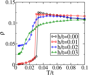
Figure 1: Colour online: The resistivity $\rho(T)$ in the absence of antisite disorder for cooling in different applied fields. For temperatures below the zero field transition, $T_{c}^{0}$, $\rho(T)$ increases on applying a field, and for $T>T_{c}^{0}$ $\rho(T)$ decreases on applying a field. The ratio $\rho(T,h)/\rho(T,0)$ can be very large as $T\rightarrow 0$ in this field cooling situation.

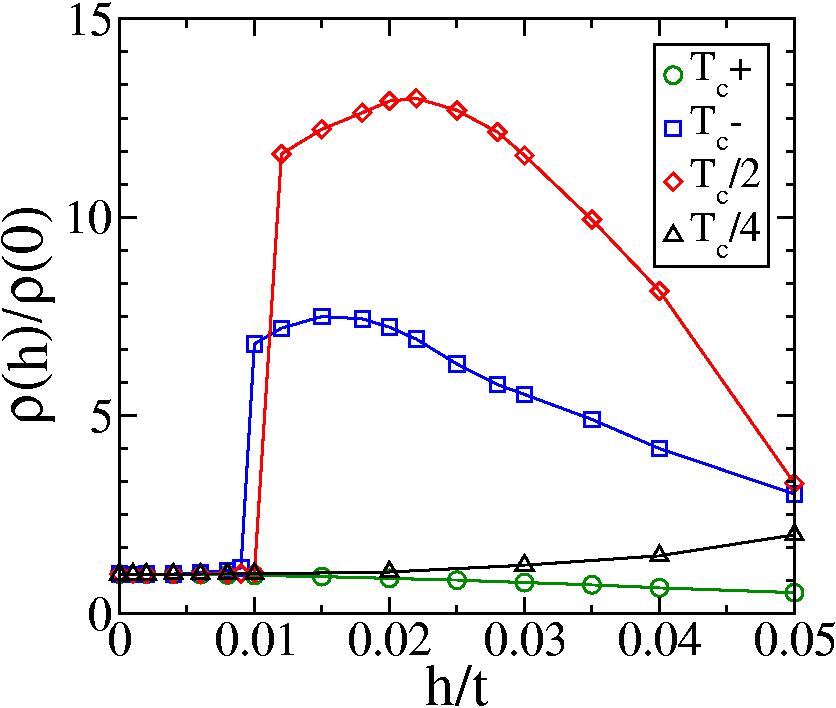
Figure 2: Colour online: The field dependence of the resistivity at different temperatures following a zero field cooling (ZFC) protocol. For $T=T_{c}^{+}$ (just above $T_{c}$) the zero field resistivity is already large and $\rho$ decreases slightly with $h$ due to suppression of spin disorder. For $T=T_{c}^{-}$ (just below $T_{c}$) and at $T_{c}/2$ there is a sharp increase in resistivity at $h/t\sim 0.01$, with a peak around $h/t\sim 0.02-0.03$ and a fall thereafter. This is consistent with the trends seen in Fig.1. At $T=T_{c}/4$ this ZFC scheme does not manage to create competing magnetic structures for $h/t\sim 0.05$, possibly due to metastability of the parent AFM pattern. The field induced switching is therefore easiest achieved between $T_{c}/2$ and $T_{c}$.

The A type pattern has two possible orientations of the stripes, either from bottom left to top right, or from bottom right to top left. These are the two ‘diagonals’ in 2D. The first corresponds to peaks in the structure factor $D({\bf q})$ at $\{{\bf Q}_{A1},{\bf Q}_{A2}\}$, and the second to peaks at $\{{\bf Q}_{A3},{\bf Q}_{A4}\}$. For reference, ${\bf Q}_{A1}=\{\pi/2,\pi/2\}$, ${\bf Q}_{A2}=\{3\pi/2,3\pi/2\}$, ${\bf Q}_{A3}=\{\pi/2,3\pi/2\}$, ${\bf Q}_{A4}=\{3\pi/2,\pi/2\}$. The ferromagnetic peaks in $S({\bf q})$ are at ${\bf Q}_{F1}=\{0,0\}$ and ${\bf Q}_{F2}=\{\pi,\pi\}$. The ordered configurations lead to peaks at two wavevectors since the model has both magnetic and non-magnetic sites and our wavevectors are defined on the overall B-B’ lattice.

Let us first examine the FC results in resistivity, Fig.1. Cooling at $h/t=0$ leads to a sharp drop in resistivity at $T=T_{c}^{0}\sim 0.032$, where $T_{c}^{0}$ is the zero field transition temperature, and $\rho(T)\rightarrow 0$ as $T\rightarrow 0$. Cooling at $h/t=0.01$ leads to a small suppression in $T_{c}$ but the trend in $\rho(T)$ remains similar to $h/t=0$. Between $h/t=0.01$ and $h/t=0.02$, however, there is a drastic change in $\rho(T)$, and, as we will see later, in the magnetic state. The primary effect is a sharp increase in the $T<T_{c}^{0}$ resistivity, with the $T\rightarrow 0$ resistivity now being almost $40\%$ of the paramagnetic value. Even at this stage it is clear that $\rho(T,h)/\rho(T,0)$ can be very large as $T\rightarrow 0$ and is $\sim 4$ for $T\sim T_{c}^{0}$ and $h/t=0.02$. Increasing the field even further leads to a reduction in $\rho(T)$ over most of the temperature window since the field promotes a ferromagnetic state suppressing the AFM fluctuations.

We can study the impact of the magnetic field also within the ZFC scheme. Fig.2 shows the result of applying a field after the cooling the system to four different temperatures, (i) $T_{c}^{+}$ (slightly above $T_{c}^{0}$), (ii) $T_{c}^{-}$ (slightly below $T_{c}^{0}$), (iii) $T_{c}^{0}/2$ and (iv) $T_{c}^{0}/4$.

For $T>T_{c}^{0}$, the applied field mainly suppresses the AFM fluctuations, leading to a gradual fall in the resistivity. This is weak negative MR. Below $T_{c}^{0}$ (where there is already noticeable AFM order) and at $T_{c}^{0}/2$ the resistivity remains almost unchanged till some value $h_{c}(T)$ and then switches dramatically. There is a peak in the ratio $\rho(T,h)/\rho(T,0)$ at $h\gtrsim 0.02$ and then a gradual decrease. At $T_{c}^{0}/2$ the ratio reaches a maximum $\sim 12$. At lower temperature, $T_{c}^{0}/4$, the field appears to have a much weaker effect, mainly because the update mechanism that we adopt does not allow a cooperative switching of the AFM state at low $T$ till very large fields. Overall, there is a window of $T$ over which a moderate magnetic field can lead to a several fold rise in resistivity.

A first understanding of the rise in resistivity can be obtained from the magnetic snapshots of the system at $T=T_{c}^{0}/2$ in Fig.3. We plot the correlation $f_{i}={\bf S}_{0}.{\bf S}_{i}$ in an equilibrium magnetic snapshot, where ${\bf S}_{0}$ is a reference spin (bottom left corner) and ${\bf S}_{i}$ is the spin at site ${\bf R}_{i}$. The left panel is at $h/t=0$ and shows a high level of A type correlation (stripe like pattern). This is a ‘low dimensional’ electron system since the electron propagation is along the one dimensional stripes in this 2D system. The stripe pattern has a high degree of order so the scattering effects and resistivity are low. The second panel is at $h/t=0.008$, just below field induced destruction of AFM order, and the pattern is virtually indistinguishable from that in the first panel.

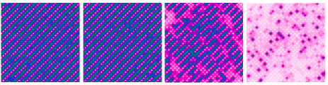
Figure 3: Colour online: Evolution of spin correlations in the clean system in response to a magnetic field. The plot shows $f_{i}={\bf S}_{0}.{\bf S}_{i}$ in magnetic snapshots at different $h$, where ${\bf S}_{0}$ is a reference spin (bottom left corner). $T=T_{c}^{0}/2$ and the fields are, from left to right, $h/t=0,~{}0.008,~{}0.02,~{}0.05$.

The third panel in Fig.3 is at $h/t=0.02$ where the applied field has suppressed long range A type order. However, there are strong A type fluctuations that persist in the system and they lead to a pattern of short range ordered A type patches with competing orientations, $\{{\bf Q}_{A1},{\bf Q}_{A2}\}$ and $\{{\bf Q}_{A3},{\bf Q}_{A4}\}$, in a spin polarised background. This patchwork leads to a high resistivity, higher than that in leftmost panel, since the ferromagnetic paths are fragmented by intervening A type regions, while the A type regions are poorly conducting due to their opposite handedness. In the last panel the field, $h/t=0.05$, is large enough so that even the AFM fluctuations are wiped out and the spin background is a 2D ferromagnet with extremely short range inhomogeneties. The resistance here is significantly below the peak value.

Let us summarise the physical picture that emerges in the non disordered system before analysing the effect of antisite disorder. The ingredients of the large MR are the following: (i) An AFM metallic phase, without too much quenched disorder so that the resistivity in the magnetically ordered state is small. (ii) Field induced suppression of the AFM order at $h=h_{c}(T)$, say, replacing the ordered state with AFM correlated spins in a FM background, leading to a high resistivity state. In contrast to the standard negative MR scenario, where an applied field pushes the system from a spin disordered state to a spin ordered state, here the applied field pushes the ordered (AFM) state towards spin disorder.

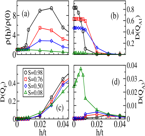
Figure 4: Colour online: Field response in the presence of antisite disorder. The temperature is $T=T_{c}^{0}/2$, where $T_{c}^{0}$ is the $T_{c}$ at $h/t=0$ in the non disordered system. The structural order parameters are indicated in panel (c), $S=1-2x$ where $x$ is the fraction of mislocated sites. The legend is same for all the panels. The results are obtained via ZFC. Panel (a) Field dependence of resistivity, normalised to $\rho$ at $h/t=0$. (b) Magnetic structure factor at the major AFM peak ${\bf Q}_{A1}$. The value is same at ${\bf Q}_{A2}$ also. (c) Growth in the FM structure factor with $h$. (d) Growth in the complementary AFM peak ${\bf Q}_{A3}$, the result is same for ${\bf Q}_{A4}$. The primary observation here is the continuation of the clean limit results, with suppressed magnitude, down to $S=0.50$.

While our concrete results are in the case of a 2D ‘double perovskite’ model and a stripe-like ground state, the principle above is far more general and should apply to other non ferromagnetic ordered states in two or three dimensions and to microscopic models that are very different from the double perovskites. We will discuss this issue at the end.

Defects are inevitable in any system and in particular one expects antisite disorder in the DP’s. The concentration of such defects may actually increase on electron doping a material like SFMO, due to the valence change, and we need to check if the large MR is wiped out by weak disorder. The presence of ASD affects the zero field magnetic state itself, as we have discussed elsewhere vn-pm-afm , and the field response has to be understood with reference to this $h/t=0$ state. Let us first define the augmented model to describe the presence of ASD.

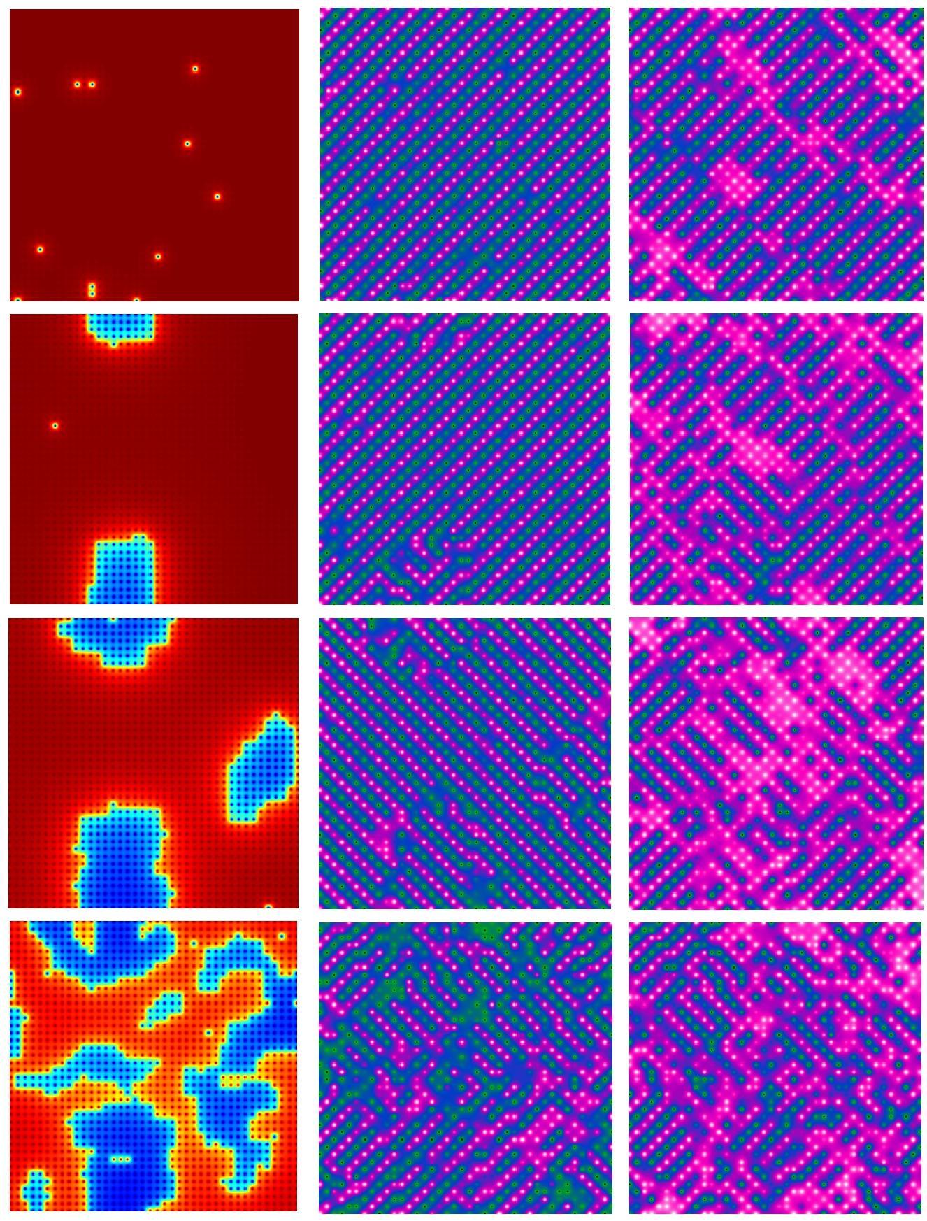
Figure 5: Colour online: Field response in the antisite disordered systems at $T=T_{c}^{0}/2$, for the $S$ values in Fig.4. The left panels indicate the structural domains in the antisite disordered systems. The middle column shows the spin correlations at $h/t=0$, note that rows 1-3 show significant A type order, while the pattern in the 4th row has AFM domains of both orientations and so suppressed long range order. The right column shows the spin correlations at $h/t=0.02$. In rows 1-3 the AFM pattern gets fragmented and FM regions show up. In row 4 the finite field pattern is not significantly different from the $h/t=0$ case. Overall, the field enhancement of ‘spin disorder’ is large in the first three cases but modest at strong ASD.

We generalise the clean model by including a configuration variable $\eta_{i}$, with $\eta_{i}=1$ for B sites and $\eta_{i}=0$ for B’ sites. In the structurally ordered DP the $\eta_{i}$ alternate along each axis. We consider progressively ‘disordered’ configurations, generated through an annealing process ps-pm-asd . These mimic the structural domain pattern observed asd-tok-dom ; asd-dd-dom in the real DP. For any specified $\{\eta\}$ background the electronic-magnetic model has the form:

$$H=H_{loc}\{\eta\}+H_{kin}\{\eta\}+H_{mag}\{\eta\}$$

$H_{loc}\{\eta\}~{}=~{}\epsilon_{B}\sum_{i}\eta_{i}f_{i\sigma}^{\dagger}f_{i\sigma}+\epsilon_{B^{\prime}}\sum_{i}\left(1-\eta_{i}\right)m_{i\sigma}^{\dagger}m_{i\sigma}$, the hopping term connects NN sites, irrespective of whether they are B or B’: $H_{kin}\{\eta\}=-t_{1}\sum_{{\langle i,j\rangle}\sigma}\eta_{i}\eta_{j}f_{i\sigma}^{\dagger}f_{j\sigma}$ $-t_{2}\sum_{{\langle i,j\rangle}\sigma}(1-\eta_{i})(1-\eta_{j})m_{i\sigma}^{\dagger}m_{j\sigma}$ $-t_{3}\sum_{{\langle i,j\rangle}\sigma}(\eta_{i}+\eta_{j}-2\eta_{i}\eta_{j})(f_{i\sigma}^{\dagger}m_{j\sigma}+h.c)$. The magnetic interactions include the Hund’s coupling on B sites, and AFM superexchange $J_{AF}=0.08t$ between two NN B sites: $H_{mag}\{\eta\}=J\sum_{i}\eta_{i}{\bf S}_{i}.f_{i\alpha}^{\dagger}{\vec{\sigma}}_{\alpha\beta}f_{i\beta}+J_{AF}\sum_{\left\langle i,j\right\rangle}\eta_{i}\eta_{j}{\bf S}_{i}\cdot{\bf S}_{j}$. For simplicity we set the NN hopping amplitudes $t_{1}=t_{2}=t_{3}=t$.

We use the simplest indicator $S=1-2x$ (not to be confused with the magnitude of the core spin), to characterise these configurations, where $x$ is the fraction of B (or B’) atoms that are on the wrong sublattice. Fig.4 shows the resistivity ratio $\rho(h)/\rho(0)$ at $T=T_{c}^{0}/2$, in panel (a), and the field dependence of structure factor peaks in panels (b)-(d). Fig.5 first column shows the structural motifs on which the magnetism is studied.

Down to $S=0.50$ the ratio $\rho(h)/\rho(0)$ has a behaviour similar to the clean case, Fig.2, but the peak ratio reduces to $\sim 3$ for $S=0.50$. There is a corresponding field induced suppression in the principal AFM peak ${\bf Q}_{A1}$ and an enhancement of the FM peak ${\bf Q}_{F}$. The complementary AF peak ${\bf Q}_{A3}$ slowly increases with $h$, has a maximum around $h/t=0.02$ (where the disconnected AFM domains exist) and falls at large $h$ as the system becomes FM overall. The trend that we had observed in the clean limit is seen to survive to significant disorder. At $S=0.08$, where the B-B’ order is virtually destroyed, the $h/t=0$ state, Fig.5 last row, has no long range AFM order. It is already a high resistivity state and an applied field actually leads to weak negative MR.

Let us place our results in the general context of AFM metals. (i) Theory: we are aware of one earlier effort af-met-th in calculating the MR of AFM metals (and semiconductors), assuming electrons weakly coupled to an independently ordering local moment system. Indeed, the authors suggested that AFM semiconductors could show positive MR. Our framework focuses on field induced suppression of long range AFM order, rather than perturbative modification, and the positive MR shows up even in a ‘high density’ electron system. The electron-spin coupling is also (very) large, $J/t\gg 1$, and cannot be handled within Born scattering.

(ii) Experiments: the intense activity on oxides has led to discovery of a few AFM metals, e.g, in the manganite La_0.46Sr_0.54MnO₃ af-met1 , in the ruthenate Ca₃Ru₂O₇ af-met2 ; af-met3 , and CaCrO₃ af-met4 . Of these Ca₃Ru₂O₇ indeed shows large increase in resistivity with field induced growth of FM order af-met3 . For the manganite and CaCrO₃ (where the resistivity is too large) we are not aware of MR results across the field driven transition. Some heavy fermion metals too have AFM character but the field driven transition affects the local moment itself, making the present scenario inapplicable.

(iii) Generalisation: the information about the spin configurations at any $(T,h)$ is encoded in the structure factor, $D({\bf q})$. Let us put down a form for $D({\bf q})$ and suggest how it affects the resistivity. To simplify notation we will assume that the AFM peak is at one wavevector ${\bf Q}$, while the FM peak is at $\{0,0\}$. The AFM phase has an order parameter $m_{AF}$, say, while, for $h>h_{c}(T)$, there is induced FM order of magnitude $m_{F}$. Assuming that the dominant fluctuations in the relevant part of the $(T,h)$ phase diagram are at ${\bf q}\sim{\bf Q}$, we can write: $D({\bf q})\sim m^{2}_{AF}\delta({\bf q}-{\bf Q})+A/(1+({\bf q}-{\bf Q})^{2}\xi^{2})$ when $h<h_{c}(T)$, and $D({\bf q})\sim m^{2}_{F}\delta({\bf q})+A^{\prime}/(1+({\bf q}-{\bf Q})^{2}\xi^{2})$ when $h>h_{c}(T)$. $m_{AF},m_{F}$ and $\xi$ depend on $(h,T)$, $A$ depends on $m_{AF}$ and $\xi$ and $A^{\prime}$ on $m_{F}$ and $\xi$. The amplitudes $A$ and $A^{\prime}$ vanish as the corresponding $m$ tend to saturate (since the spins get perfectly ordered). The delta functions $D({\bf q})$ dictate the bandstructure while electron scattering is controlled by the Lorentzian part.

Consider three cases (a) $T=T_{c}^{+},~{}h=0$, (b) $T=T_{c}^{-},~{}h=0$, and (c) $T=T_{c}^{-},~{}h>h_{c}(T)$. In (a) there is no order, so A is large, and $\rho=\rho_{a}$, say. For (b) even if $\xi$ were the same as in (a), the presence of a large order parameter would suppress $A$ and hence the scattering. We call this $\rho=\rho_{b}<<\rho_{a}$ (assuming there is indeed a large order parameter and no significant background resistivity due to impurities). If we apply a field such that $m_{AF}\rightarrow 0$ but $m_{F}$ is still small, then the structure factor crudely mimics the paramagnetic case, and we should have $\rho_{c}\approx\rho_{a}$. If all this is true, then just beyond field suppression of AFM order (and for $T$ just below $T_{c}$) we should get $\rho_{c}/\rho_{b}\gg 1$. Broadly, if the appearance of AFM order with reducing $T$ leads to a sharp drop in $\rho$ then the field induced resistivity ratio can be large. This is independent of dimensionality and microscopic detail. A caution: as $T\rightarrow 0$, the applied field would drive a first order transition from a large $m_{AF}$ state to one with large $m_{F}$ and weak scattering. The scenario above will not work, as our Fig.2 illustrated.

Conclusion: We have studied the magnetoresistance in an antiferromagnetic metal motivated by the prediction of such a phase in the double perovskites. Beyond the modest field needed for suppression of long range antiferromagnetic order, the system shows almost tenfold increase in resistivity near $T_{c}$. The effect originates from strong antiferromagnetic fluctuations in the field induced ferromagnetic background. The large positive magnetoresistance, though suppressed gradually, survives the presence of significant antisite disorder. The principle that we uncover behind this ‘colossal positive magnetoresistance’ should be applicable to other local moment based AFM metals as well.

Acknowledgments: We acknowledge use of the Beowulf Cluster at HRI, and thank S. Datta and G. V. Pai for discussions. PM acknowledges support from a DAE-SRC Outstanding Research Investigator Award, and the DST India (Athena).

References

- (1) R. von Helmolt et al., Phys. Rev. Lett. 71, 2331 (1993).
- (2) Y. Shimikawa et al., Nature (London) 379, 53 (1996).
- (3) G. Petrich et al., Phys. Rev. Lett 26 885 (1971).
- (4) For reviews, see D. D. Sarma, Curr. Op. Sol. St. Mat. Sci.,5, 261 (2001), D. Serrate et al., J. Phys. Cond. Matt. 19, 023201 (2007).
- (5) T. Akimoto et al., Phys. Rev. B57, 5594 (1998).
- (6) X. N. Lin et al., Phys. Rev. Lett. 95, 017203 (2005).
- (7) Y. Yoshida et al., Phys. Rev. B72, 054412 (2005).
- (8) A. C. Komarek et al., Phys. Rev. Lett. 101, 167204 (2008).
- (9) K.-I. Kobayashi et al., Nature 395, 677 (1998).
- (10) Y. H. Huang et al., Phys. Rev. B73, 104408 (2006), Y. H. Huang et al., Phys. Rev. B74, 174418 (2006).
- (11) J. Navarro et al., J. Phys. Cond. Matt 13, 8481 (2001), J. Navarro et al., Phys. Rev. B67, 174416 (2003).
- (12) E. Dagotto, Science, 309, 257 (2005).
- (13) P. Sanyal and P. Majumdar, Phys. Rev. B80, 054411 (2009).
- (14) P. Sanyal et al., Phys. Rev. B80, 224412 (2009).
- (15) R. Tiwari and P. Majumdar, arXiv:1105.0148.
- (16) D. Sanchez et al., J. Mater. Chem. 13, 1771 (2003).
- (17) S. Ray et al., unpublished.
- (18) V. Singh and P. Majumdar, arXiv. 1009.1709.
- (19) S. Kumar and P.Majumdar, Eur. Phys. J. B50, 571 (2006)
- (20) P. Sanyal et al., Eur. Phys. J. B65, 39 (2008).
- (21) T. Asaka et al., Phys Rev B75, 184440 (2007).
- (22) C. Meneghini et al., Phys. Rev. Lett. 103, 046403 (2009).
- (23) I. Balberg and J. S. Helman, Phys. Rev. B18, 303 (1978).