Deformed triangular lattice antiferromagnets in a magnetic field: role of spatial anisotropy and Dzyaloshinskii-Moriya interactions

Abstract

Recent experiments on the anisotropic spin-1/2 triangular antiferromagnet Cs₂CuBr₄ have revealed a remarkably rich phase diagram in applied magnetic fields, consisting of an unexpectedly large number of ordered phases. Motivated by this finding, we study the role of three ingredients—spatial anisotropy, Dzyaloshinskii-Moriya interactions, and quantum fluctuations—on the magnetization process of a triangular antiferromagnet, coming from the semiclassical limit. The richness of the problem stems from two key facts: 1) the classical isotropic model with a magnetic field exhibits a large accidental ground state degeneracy, and 2) these three ingredients compete with one another and split this degeneracy in opposing ways. Using a variety of complementary approaches, including extensive Monte Carlo numerics, spin-wave theory, and an analysis of Bose-Einstein condensation of magnons at high fields, we find that their interplay gives rise to a complex phase diagram consisting of numerous incommensurate and commensurate phases. Our results shed light on the observed phase diagram for Cs₂CuBr₄ and suggest a number of future theoretical and experimental directions that will be useful for obtaining a complete understanding of this material’s interesting phenomenology.

I Introduction

Antiferromagnetic spin models on the triangular lattice constitute one of the simplest and most widely studied realizations of geometric frustration. Indeed, the Ising triangular antiferromagnet was the first spin model found to possess a disordered ground state and extensive residual entropyWannier (1950) at zero temperature ($T$). While the classical Heisenberg model on the triangular lattice does order at $T=0$ into a well-known commensurate spiral pattern (also known as a $\sqrt{3}\times\sqrt{3}$ state), the fate of the quantum spin-1/2 Heisenberg Hamiltonian has been the subject of a long and fruitful debate spanning over 30 years of research. Although the originally proposed resonating valence bond liquid Anderson (1973); Fazekas and Anderson (1974) did not emerge as the ground state of the spin-1/2 Heisenberg model Huse and Elser (1988); Bernu et al. (1992); Capriotti et al. (1999), such a phase was later found in a related quantum dimer model on the triangular lattice Moessner and Sondhi (2001).

Triangular antiferromagnets in an applied magnetic field—which is our focus here—have also been extensively studied for decades, and found to possess unusual magnetization physics which remains only partially understood. Underlying much of this interesting behavior is the discovery, made long ago Kawamura and Miyashita (1984), that in a magnetic field Heisenberg spins with isotropic exchange interactions exhibit a large accidental classical ground state degeneracy. That is, at finite magnetic fields there exists an infinite number of continuously deformable classical spin configurations which constitute minimum energy states, but are in no way symmetry related. As reviewed later, this degeneracy is lifted by thermal (finite $T$) Kawamura and Miyashita (1984) and quantum (finite spin $S$) Chubukov and Golosov (1991) fluctuations; such fluctuation-driven selection, also known as order-by-disorderShender (1982); Henley (1989), results in a nontrivial temperature-field phase diagram Kawamura and Miyashita (1984) consisting of three ordered phases. In particular, coplanar ‘Y’ and ‘V’ states are separated by a collinear up-up-down (UUD) phase which realizes, for finite spin $S$ and at $T=0$, a one-third magnetization plateau over a finite field interval. This plateau state preserves continuous spin rotation symmetry about the magnetic field direction and is remarkably stable: unlike all other magnetically-ordered states it survives “dimensional reduction” and exists even in the smallest possible triangular lattice strip, the two-chain zig-zag ladder Okunishi and Tonegawa (2003); Hikihara et al. (2010).

To date a large number of magnetic materials have been synthesized that realize triangular antiferromagnets, and experiments on such compounds have highlighted the spectacular breadth of phenomena that can be driven by the interplay between magnetic fields and geometric frustration stemming from the lattice. For example, a stacked triangular antiferromagnet with weak inter-plane coupling is realized by the $S=5/2$ material RbFe(MoO₄)₂, whose phase diagramSvistov et al. (2006) features all of the fluctuation-selected states discussed above. Reducing the magnitude of the magnetic ion’s spin enhances quantum fluctuations, sometimes leading to highly non-classical behavior. Low-spin materials which constitute ‘deformed’ triangular antiferromagnets—that is, with spatially anisotropic exchange interactions that are not SU(2) symmetric—have indeed provided numerous surprises which are very likely quantum in origin. Studies of the spin-1/2 compounds Cs₂CuCl₄ and Cs₂CuBr₄ have been particularly fruitful in this regard. Inelastic neutron scattering has revealed striking dominance of a multi-particle continuum in the dynamical response of Cs₂CuCl₄ Coldea et al. (2002, 2003). This continuum is naturally explained in terms of spin-1/2 spinon excitations of weakly coupled chains. Ordered phases of this material show strong sensitivity to the magnitude and direction of the external magnetic field Tokiwa et al. (2006). The complexity of the $h-T$ phase diagram has been attributed to the competition between several asymmetric exchanges of the Dzyaloshinskii-Moriya (DM) type and a weak inter-plane exchange interaction. In particular it has been suggested Starykh et al. (2010) that, although weak, inter-plane exchange can dominate over stronger but frustrated inter-chain coupling and dictate the type of three-dimensional magnetic ordering at low temperatures.

Our study here is strongly motivated by the isostructural material Cs₂CuBr₄, whose triangular planes are less anisotropic and exhibit weaker inter-plane coupling compared to Cs₂CuCl₄, leading to rather different but equally rich phenomenology in magnetic fields. With fields directed in the plane of the triangular layers, the experimentally determined phase diagram for Cs₂CuBr₄ hosts as many as nine phases Fortune et al. (2009) at low temperature. A one-third magnetization plateau features very prominently Ono et al. (2003); Tsujii et al. (2007); Fujii et al. (2007) amongst the other, less understood, phases and offers a convenient starting point for theoretical analysis Alicea et al. (2009). Notably, Cs₂CuCl₄ shows no signs of this plateau, which has been attributed Starykh et al. (2010) to its more pronounced spatial anisotropy and stronger inter-layer couplingOno et al. (2005); Foyevtsova et al. (2011), which is known to suppress the plateau Gekht and Bondarenko (1997). And unlike the higher-spin material RbFe(MoO₄)₂ discussed above Svistov et al. (2006), the width of the magnetization plateau in Cs₂CuBr₄ is essentially $T$-independent Tsujii et al. (2007), strongly hinting at its quantum origin.Chubukov and Golosov (1991); Alicea et al. (2009); Tay and Motrunich (2010)

The sheer number of states present in the phase diagram of Cs₂CuBr₄, in comparison with the three phases expected from the standard isotropic Heisenberg antiferromagnet on the triangular lattice, make it clear that a thorough theoretical study is required to begin understanding this material’s complex behavior. Here we attempt to access the global phase diagram of this system by analyzing the roles of three important known perturbations away from the ‘ideal’ classical triangular antiferromagnet—quantum fluctuations stemming from the low spin $S=1/2$, spatial exchange anisotropy, and Dzyaloshinskii-Moriya (DM) interactions—all of which compete and favor different spin arrangements. Because the ideal classical model exhibits a large ground state degeneracy, we show that even weak spatial anisotropy and DM coupling are sufficient to qualitatively alter the standard Y-UUD-V phase diagram, stabilizing new spin orders including incommensurate ‘umbrella’ and planar states, a commensurate ‘distorted V’ spin structure, and a commensurate ‘inverted Y’ phase. Further experiments (such as neutron scattering and NMR measurements) will be very helpful for identifying which of these orders appear in the observed phase diagram, thereby sharpening the outstanding theoretical questions that undoubtedly remain. We also predict that—in sharp contrast to Cs₂CuCl₄—the phase diagram of Cs₂CuBr₄ ought to be insensitive to the direction of the magnetic field inside of the triangular planes.

The remainder of the paper is organized as follows. We provide an overview of the model and strategy that we pursue in Sec. II, and review the physics of the isotropic triangular antiferromagnet in Sec. III. Section IV addresses the case where DM coupling is present but spatial exchange anisotropy is neglected. We then explore the Bose-Einstein condensation of magnons near the saturation field in Sec. V, which allows us to simultaneously treat quantum fluctuations, DM coupling, and spatial anisotropy in a simple setting. The influence of spatial anisotropy on the global phase diagram is studied with and without DM interactions in Secs. VI and VII, respectively. Finally, we provide a summary and concluding remarks in Sec. VIII.

II Model and Strategy

We study the following Hamiltonian,

$$H = \sum_{\langle{\bf rr^{\prime}}\rangle}J_{{\bf r,r^{\prime}}}{\bf S}_{\bf r}\cdot{\bf S}_{\bf r^{\prime}}-\sum_{r}{\bf h}\cdot{\bf S}_{\bf r}+H_{\rm{DM}}$$ (1)

where the exchange integral $J_{\bf r,r^{\prime}}$ is given by $J$ on the horizontal bonds and $J^{\prime}$ on the diagonal zig-zag bonds as shown in Fig. 1. For Cs₂CuBr₄, experiments have measured the valuesTsujii et al. (2007) $J=11.3K$ and $J^{\prime}=8.3K$. The second term describes the Zeeman energy of spins in an external magnetic field while the third, $H_{\rm{DM}}$, represents the asymmetric DM interaction between neighboring spins.

Ideally, one would like to obtain the phase diagram for the quantum spin-1/2 problem above to begin understanding the interesting phenomenology of Cs₂CuBr₄. In this paper we will attempt to access the physics of the spin-1/2 system coming from the large-$S$ limit, including quantum fluctuations perturbatively. This nevertheless still leaves a problem of substantial complexity, which can be understood by considering the classical, spatially isotropic limit of $H$, without DM coupling. Let us denote this minimal classical Hamiltonian by $H_{0}$. As noted in the introduction and reviewed in detail in Sec. III, at finite magnetic fields $H_{0}$ exhibits a large ‘accidental’ ground state degeneracy. Quantum fluctuations (and thermal fluctuations at finite temperature) lift this ground state degeneracy, as do spatial anisotropy and DM coupling. However, all of these ingredients compete with one another, favoring completely different ordered states. To resolve this competition, our strategy will be to compute the lowest-order energy splittings for the degenerate ground states of $H_{0}$ coming from each effect. As we will see later quantum fluctuations and DM interactions split this degeneracy already at first order, while spatial anisotropy achieves this only at second order. Thus despite the fact that in Cs₂CuBr₄ spatial anisotropy [as quantified by $(J-J^{\prime})\sim 0.3J$] is expected to greatly exceed the characteristic energy scales for DM interactions in the material, the two can in fact comparably influence the phase diagram.

An additional complication arises from the fact that crystal symmetry of Cs₂CuBr₄ permits several DM terms Starykh et al. (2010) which together break the SU(2) spin symmetry enjoyed by the exchange coupling down to a discrete subgroup. One might then expect the phase diagram to depend sensitively both on the polar angle that ${\bf h}$ makes with respect to the $z$-axis, normal to the triangular plane, and the azimuthal angle ${\bf h}$ makes in the $(x,y)$ plane. Such a highly anisotropic phase diagram indeed emerges in the more spatially anisotropic materialTokiwa et al. (2006) Cs₂CuCl₄. In the limit of weak spatial anisotropy—which due to the relevance to Cs₂CuBr₄ is our main focus here—most of these DM couplings fortunately play an unimportant role. As justified in Appendix A, it indeed suffices to consider only

$$H_{\rm{DM}}=-\sum_{{\bf r}}{\bf D}\cdot\left[{\bf S}_{\bf r}\times({\bf S}_{{\bf r}+\bm{\delta}_{1}}+{\bf S}_{{\bf r}+\bm{\delta}_{3}})\right],$$ (2)

where the DM vector is ${\bf D}=D{\bf\hat{z}}$ (we assume $D>0$ throughout) and $\bm{\delta}_{1,3}$ are vectors shown in Fig. 1. The strength of this DM interaction is expected to be comparable to that in the isostructural material Cs₂CuCl₄, whereColdea et al. (2002) $D\approx J/20$.

Notice that at ${\bf h=0}$ the model with the above DM coupling still exhibits a U(1) spin symmetry corresponding to global spin rotations about the ${\bf D}$ vector. This leads to a major simplification—the phase diagram of $H$ depends on the polar angle ${\bf h}$ makes with the $z$-direction but not on the azimuthal angle. All additional DM terms which lower this symmetry lift the accidental degeneracy of $H_{0}$ only at second order in their couplings, whereas $H_{\rm DM}$ above has a first-order effect; see Appendix A for details. We emphasize that a nontrivial consistency check emerges here regarding relevance of our results to experiments on Cs₂CuBr₄. Our approach postulates that the physics of this material can be accessed coming from the classical, isotropic model without DM coupling. If this postulate is correct, then contrary to Cs₂CuCl₄, the experimental phase diagram of Cs₂CuBr₄ should be qualitatively insensitive to rotations of the field about the ${\bf\hat{z}}$ direction. Recent experiments by Y. Takano and collaborators Takano (2011) have indeed shown that the low-temperature phase diagram of Cs₂CuBr₄ is qualitatively the same for fields oriented along the material’s ${\bf b}$ and ${\bf c}$ axes ($x$ and $y$ axes in our notation from Fig. 1). This finding lends strong experimental support to our approach.

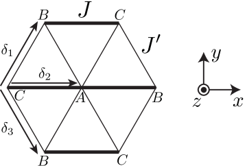
Figure 1: Spatially anisotropic triangular lattice with exchange $J$ along horizontal bonds and $J^{\prime}$ along diagonal bonds. We define axes such that the sites lie in the $(x,y)$ plane as shown. Vectors ${\bm{\delta}}_{1,2,3}$ connect nearest-neighbor sites of the lattice. In the isotropic limit where $J=J^{\prime}$ and Dzyaloshinskii-Moriya coupling is absent, the Hamiltonian in Eq. (1) exhibits a highly degenerate classical ground state manifold wherein spins order in an underconstrained three-sublattice pattern. We label the three sublattices by $A,B$, and $C$.

III Review of the Isotropic Model: $J=J^{\prime},D=0$

III.1 Classical ground states

In the absence of DM coupling, the classical isotropic Heisenberg model, where spins are described as 3D unit vectors, is well known to exhibit a large ‘accidental’ ground state degeneracy in applied magnetic fields Kawamura and Miyashita (1984). The classical ground state structure can be conveniently exposed by expressing the Hamiltonian (up to a constant) as

$$H_{0}=\frac{J}{2}\sum_{\bf r}\left[{\bf M}_{\Delta}({\bf r})-\frac{\bf h}{3J}\right]^{2},$$ (3)

where

$${\bf M}_{\Delta}({\bf r})={\bf S}_{\bf r}+{\bf S}_{{\bf r}+\bm{\delta}_{1}}+{\bf S}_{{\bf r}+\bm{\delta}_{2}}$$ (4)

represents the magnetization of an elementary triangle located at site ${\bf r}$. Below the saturation field $h_{\rm sat}^{0}=9J$, it is clear from Eq. (3) that classical ground states satisfy the condition ${\bf M}_{\Delta}({\bf r})={\bf h}/(3J)$ for all ${\bf r}$. States fulfilling this requirement exhibit a three-sublattice structure as shown in Fig. 1, whose spins ${\bf S}_{A,B,C}$ are determined from

$${\bf S}_{A}+{\bf S}_{B}+{\bf S}_{C}=\frac{{\bf h}}{3J}.$$ (5)

The ground state degeneracy follows immediately from Eq. (5), since the spins on the three sublattices are specified by a total of six angles which are constrained by only three equations. Parametrizing the spins on sublattice $\alpha$ as

$${\bf S}_{\alpha}=(\sin\theta_{\alpha}\cos\phi_{\alpha},\sin\theta_{\alpha}\sin\phi_{\alpha},\cos\theta_{\alpha}),$$ (6)

the angles must specifically satisfy

$$\frac{{\bf h}\cdot{\bf\hat{x}}}{3J} = \sin\theta_{A}\cos\phi_{A}+\sin\theta_{B}\cos\phi_{B}+\sin\theta_{C}\cos\phi_{C}$$

$$\frac{{\bf h}\cdot{\bf\hat{y}}}{3J} = \sin\theta_{A}\sin\phi_{A}+\sin\theta_{B}\sin\phi_{B}+\sin\theta_{C}\sin\phi_{C}$$

$$\frac{{\bf h}\cdot{\bf\hat{z}}}{3J} = \cos\theta_{A}+\cos\theta_{B}+\cos\theta_{C}$$ (7)

Equations (7) allow one to, say, express $\phi_{B},\phi_{C}$, and $\theta_{C}$ in terms of $\phi_{A},\theta_{A}$, and $\theta_{B}$. Note, however, that classical ground states do not exist for all possible values of the latter angles.

At ${\bf h}=0$ where the classical Hamiltonian exhibits O(3) symmetry, this degeneracy is symmetry-related: the three unconstrained angles reflect the arbitrariness of the plane in which the $120^{\circ}$ spiral orients and the freedom for rotating all spins by an arbitrary angle within that plane. Introducing a finite magnetic field reduces the spin symmetry down to U(1). The three free angles nevertheless persist, only one of which is now symmetry-related (corresponding to global rotations of the spins about the magnetic field axis). Consequently, in finite magnetic fields below saturation, $H_{0}$ exhibits an accidental classical ground state degeneracy specified by two continuously deformable angles. Figure 2 illustrates some important members of this ground state manifold which we will frequently refer to later on: (a) Y, (b) up-up-down (UUD), (c) V, (d) ‘distorted V’, (e) ‘inverted Y’, and (f) umbrella states.

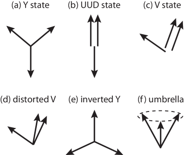
Figure 2: Important members of the classical ground state manifold exhibited by Eq. (1) when $J=J^{\prime}$ and Dzyaloshinskii-Moriya coupling is absent: (a) Y, (b) up-up-down (UUD), (c) V, (d) ‘distorted V’, (e) ‘inverted Y’, and (f) umbrella states. The arrows denote the spin orientations on the $A$, $B$, and $C$ sublattices of Fig. 1.

III.2 Symmetries of the classical ground states

It is important to emphasize the symmetry distinction between the above phases. Because $\langle{\bf S}_{\bf r}\cdot{\bf h}\rangle$ is uniform in umbrella configurations, this order is exceptional among the classical ground states in that it preserves the original lattice translation symmetry [when followed by an appropriate global U(1) spin rotation]. All other classical ground states exhibit a nontrivial three-sublattice pattern of $\langle{\bf S}_{\bf r}\cdot{\bf h}\rangle$ and therefore spontaneously break discrete translation symmetry. UUD order is also exceptional—it alone preserves global U(1) spin rotations about the field axis and therefore does not break any continuous symmetry. Ultimately, the U(1) spin symmetry enjoyed by the UUD state permits the formation of a one-third magnetization plateau in this system. In a boson representation of the spins, umbrella order corresponds to a superfluid phase, UUD order is a solid phase, and all other classical ground states constitute supersolids.Heidarian and Damle (2005); Jiang et al. (2009); Wang et al. (2009)

These ‘supersolids’ can be further distinguished by symmetry. Since in the V state spins on two sublattices, say A and B, are parallel, this order is symmetric under spatial $\pi/3$ rotations about a site on the C sublattice. This can also be phrased as invariance of the V state with respect to permutation of the A and B sublattices. The distorted V state, while smoothly connected to the V state, violates this symmetry (the A and B sublattices are not equivalent anymore) and therefore constitutes a distinguishable phase in the isotropic system. Finally, in both the Y and inverted-Y states spins on one sublattice, say C, point either along or against the field, and both orders are invariant under $\pi/3$ rotations about a site on sublattice C followed by a global $\pi$ spin rotation. While the latter phases exhibit identical symmetries, one can not deform the spins smoothly from one configuration to the other without breaking additional symmetries; thus it is still meaningful to classify them as different states.

All of the orders displayed in Fig. 2 thus constitute distinct phases when the full symmetries of the isotropic Heisenberg triangular antiferromagnet in field are present. Note, however, that when the symmetry is lowered by including DM coupling and/or spatial anisotropy, this ceases to be the case. The V and distorted V states, for example, are not distinguishable once $\pi/3$ rotation symmetry is removed by adding either of these ingredients. Similarly, the distinction between the UUD and Y states hinges on U(1) spin symmetry and rotation symmetry, both of which are lost in the presence of DM coupling when the magnetic field has a finite component in the $(x,y)$ plane. The UUD and distorted V states can, by contrast, remain distinct even in this physical situation, despite the very low symmetry remaining for the problem. For example, when ${\bf h}=h{\bf\hat{x}}$ and DM coupling is non-zero the Hamiltonian remains invariant under $S^{x}_{\bf r}\rightarrow S^{x}_{-\bf r}$ and $S^{y,z}_{\bf r}\rightarrow-S^{y,z}_{-\bf r}$; the UUD state respects this discrete symmetry while the distorted V state does not. We will return to these issues in subsequent sections of the paper.

III.3 Influence of thermal fluctuations

Thermal fluctuations provide one mechanism that lifts the large accidental ground state degeneracy of the classical model. At finite temperature the system minimizes its free energy, $F=U-TS$, and although the ground states exhibit identical energies $U$, their entropies generically differ. Thus only the most entropically favored states emerge. The finite temperature phase diagram was established long agoKawamura and Miyashita (1984), and is reproduced with our numerics in Fig. 3.

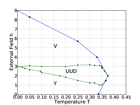
Figure 3: (Color online) Phase diagram of the classical isotropic model. Amongst the large set of accidentally degenerate classical ground states, thermal fluctuations select the Y, UUD, and V states illustrated in Figs. 2(a) through (c).

This set of Monte-Carlo simulations is based on ALPS code.Albuquerque et al. (2007) System sizes ranged from $24\times 24$ to $96\times 96$ with most simulations being carried out on $48\times 48$ lattices. (The triangular lattice can be viewed as a square lattice with bonds along one diagonal; the system sizes above refer to the dimensions of such a square lattice. All simulations were performed with periodic boundary conditions.) Every $(T,h)$ coordinate was simulated using the standard Metropolis algorithm, with 500,000 Monte Carlo steps for thermalization and another 500,000 for measurement in the $24\times 24$ system. For $48\times 48$ lattices these numbers were in the range $150,000-250,000$. All Monte Carlo data presented here and below correspond to $J=1$. Different phases and boundaries between them have been identified by the behavior of the specific heat, the magnetization $M$ and its field derivative $dM/dh$, and the vector chirality ${\bm{\kappa}}$ and coplanarity $K$ defined below.

The vector chirality is defined as

$${\bm{\kappa}} = \frac{2}{3\sqrt{3}}\frac{1}{N}\sum_{\bf{r}}\Big{(}{\bf S}_{\bf r}\times{\bf S}_{{\bf r}+\bm{\delta}_{1}}+$$ (8)

$$+{\bf S}_{{\bf r}+\bm{\delta}_{1}}\times{\bf S}_{{\bf r}+\bm{\delta}_{2}}+{\bf S}_{{\bf r}+\bm{\delta}_{2}}\times{\bf S}_{\bf r}\Big{)},$$

where $N$ is the total number of spins in the system and the normalization factor ensures that the maximal chirality magnitude is unity. Taking ${\bf h}=h{\bf\hat{z}}$ for concreteness in the remainder of this section, it is useful to consider the longitudinal $\kappa_{z}$ and transverse $\kappa_{\perp}=(\kappa_{x}^{2}+\kappa_{y}^{2})^{1/2}$ components of the vector chirality, in addition to its magnitude $\kappa=(\kappa_{z}^{2}+\kappa_{\perp}^{2})^{1/2}$. Finite longitudinal chirality $\kappa_{z}$ identifies non-coplanar spin structures of umbrella type while a non-zero transverse chirality signifies coplanar ordering in which no two spins in the unit cell are parallel (such as Y states). Notice that by construction the chirality vanishes in three-sublattice states containing two parallel spins, such as the UUD and V states.

The coplanarity $K$, introduced in Ref. Watarai et al., 2001, provides another useful indicator of planar spin structures. This quantity follows from the $A/B/C$ sublattice magnetizations

$${\bf M}_{A/B/C}=\frac{1}{N}\sum_{{\bf r}\in A/B/C}{\bf S}_{\bf r}$$ (9)

by constructing

$${\bf K}_{AB}=({\bf M}_{A}\times{\bf M}_{B})\times{\bf\hat{h}}$$ (10)

and similarly for ${\bf K}_{BC}$ and ${\bf K}_{CA}$. The coplanarity is then given by the combination

$$K^{2}=|{\bf K}_{AB}|^{2}+|{\bf K}_{BC}|^{2}+|{\bf K}_{CA}|^{2}.$$ (11)

As defined $K$ is finite for any coplanar spin configuration which includes the magnetic field in its plane. In particular, $K$ is finite in the V state but vanishes in the collinear UUD configuration.

Our Monte-Carlo simulations, summarized in Fig. 3, agree well with existing data Kawamura and Miyashita (1984); Gvozdikova et al. (2011) and clearly demonstrate entropic selection of the Y, UUD, and V states over non-coplanar order. This is consistent with the usual intuition that entropy disfavors non-coplanar structures and favors coplanar and, when available, collinear orderingShender (1982); Henley (1989). Coplanarity of the selected states is reflected in an exceedingly small value of the longitudinal chirality $\kappa_{z}$ over the entire magnetic field range $0\leq h\leq 9J$. Figures 4 and 4 exhibit the magnetization $M$ and its field derivative, $dM/dh$, at $T=0.2J$ over the same field range. Notice that the UUD state is very well identified by the abrupt variation of $dM/dh$, with two peaks in Fig. 4 representing the lower and upper critical fields. Away from the UUD state the slope of the magnetization approaches $1/(9J)$, which is just the uniform susceptibility of the classical antiferromagnet at zero temperature. The magnetization slope in the UUD state [Fig. 4] is visibly smaller, but clearly remains finite. This is a manifestation of the ‘dual’ role played by temperature: it simultaneously selects coplanar states and thermally disorders them, eventually resulting in a paramagnetic state above a field-dependent critical temperature.

Despite being such a well-studied problem, there remains a serious question about the phase diagram of the isotropic triangular lattice antiferromagnet at ${\bf h}=0$. As described above in Sec. III.1, the large degeneracy of the model in this limit is symmetry related and reflects arbitrariness of the ordering plane in which $120^{\circ}$ spiral forms. This makes the order parameter space isomorphic to SO(3), the group of rotations of a three-dimensional rigid body Kawamura and Miyashita (1984). According to the Mermin-Wagner theorem, this continuous symmetry cannot be broken at any finite temperature. Nonetheless Monte-Carlo simulations, including ours, do show a weak peak in specific heat at finite temperature, approximately $0.33J$. It has been suggested Kawamura and Miyashita (1984) that this finite-T feature in fact reflects a non-trivial phase transition associated with binding of Z₂ vortices permitted by the SO(3) structure. At present our study, which aims to understand the global features of the deformed Heisenberg model at finite $T$ and ${\bf h}$, has nothing to add to this interesting issue Wintel et al. (1995); Kawamura and Yamamoto (2007); Melchy and Zhitomirsky (2009); Kawamura et al. (2010); Okubo and Kawamura (2010); Gvozdikova et al. (2011), the resolution of which requires more extensive Monte-Carlo simulations.

We should emphasize, however, that at finite magnetic fields the entropically selected states break translational symmetry and introduce three inequivalent sublattices A, B and C. Consequently, at any finite ${\bf h}$ up to saturation there exists a finite critical temperature $T_{\rm d}$ arising from discrete symmetry breaking associated with the spontaneous selection of the sublattice ordering. In Fig. 3 this hull-shaped $T_{\rm d}(h)$ separates low-temperature ordered states from a high-temperature paramagnetic phase in which only the uniform magnetization $M$ is present.

The finite-field situation contains yet another unresolved issue, related to the U(1) symmetry corresponding to rotations about the magnetic field direction. The coplanar Y and V states break this symmetry by selecting an ordering direction in the plane perpendicular to the field direction. While due to dimensionality the U(1) symmetry can not be truly broken at finite temperature, there exists a Kosterlitz-Thouless (KT) temperature $T_{\rm KT}$ below which the transverse magnetic order exhibits power-law correlations. In principle one could have $T_{\rm KT}\neq T_{\rm d}$ (see Ref. Melchy and Zhitomirsky, 2009 for a recent example of such behavior). From the available data, however, it appears that within our numerical accuracy the two transitions coincide, $T_{\rm KT}=T_{\rm d}$. A related issue is that at finite temperature, the transitions from UUD to either Y or V are also of KT type, and as such are inherently broad and difficult to locate precisely in numerics Seabra et al. (2011). We would like to emphasize again that our main focus is on identifying possible phases rather than studying the nature of the transitions between them. Readers interested in properties of such phase transitions in a similar context are instead referred to the recent detailed study in Ref. Seabra et al., 2011.

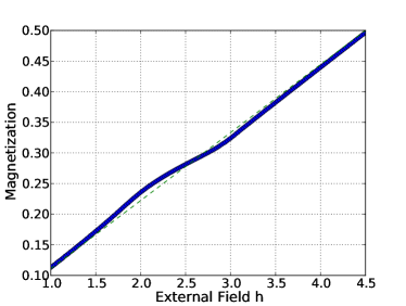
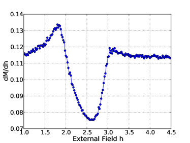
Figure 4: (Color online) (a) Magnetization $M$ and (b) its field derivative $dM/dh$ in the vicinity of one-third magnetization. The data were obtained with Monte Carlo simulations of the classical isotropic model at temperature $T=0.2J$. The collinear UUD state underlies the drop in magnetic susceptibility near $h=2.5J$, visible in both (a) and (b). The dashed line in (a) shows the $T=0$ magnetization of the classical triangular antiferromagnet, $M=h/(9J)$.

III.4 Quantum ground states

As first shown by Chubukov and GolosovChubukov and Golosov (1991), the accidental degeneracy inherent in the classical isotropic model can be lifted even at zero temperature by quantum fluctuations. Here zero-point energy of spin waves—rather than entropy—provides the degeneracy-lifting mechanism. Quantum ground state selection can be systematically explored using the machinery of the $1/S$ expansion. To this end, one starts with a particular classical ground state in the degenerate manifold and defines rotated spin coordinates $\tilde{\bf S}_{A/B/C}({\bf r})$ on the three sublattices such that the classical order corresponds to $\langle\tilde{\bf S}_{A/B/C}({\bf r})\rangle=S{\bf\hat{z}}$. One then introduces Holstein-Primakoff bosons $a({\bf r}),b({\bf r})$, and $c({\bf r})$ to express the rotated spin operators to leading order in $1/S$ as

$$\tilde{S}_{A}^{x}({\bf r}) = \sqrt{\frac{S}{2}}[a({\bf r})+a^{\dagger}({\bf r})]$$

$$\tilde{S}_{A}^{y}({\bf r}) = i\sqrt{\frac{S}{2}}[a({\bf r})-a^{\dagger}({\bf r})]$$

$$\tilde{S}_{A}^{z}({\bf r}) = S-a^{\dagger}({\bf r})a({\bf r})$$ (12)

and similarly for $\tilde{\bf S}_{B/C}({\bf r})$. Retaining only the leading-order terms in $1/S$ generates a Hamiltonian of the form $H=E_{0}+H_{2}$, where $E_{0}$ is the classical ground state energy and $H_{2}$ is quadratic in the three boson fields.

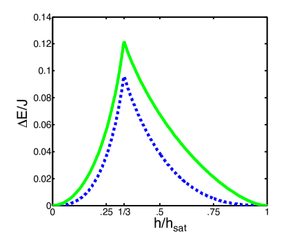
Figure 5: (Color online) Leading $1/S$ quantum energy splittings between the Y/UUD/V states and the inverted-Y (dashed line) and umbrella states (solid line). These curves illustrate an important trend — quantum fluctuations are most effective at splitting the accidental degeneracy near 1/3 magnetization where low-energy collinear states are available.

Although at a given magnetic field $h$, $E_{0}$ is identical for all allowed classical ground states satisfying Eqs. (7), the spin-wave Hamiltonian $H_{2}$ does depend on the particular ordered configuration around which one is expanding, via the dependence of the spin-wave dispersion $\omega_{k}$ on the angles $\theta_{A/B/C}$ and $\phi_{A/B/C}$. The zero-point energy for spin-waves, $\langle H_{2}\rangle=(1/2)\sum_{k}\omega_{k}$, therefore yields a $1/S$ correction to the energy that lifts the classical degeneracy. See, for example, Ref. Nikuni and Shiba, 1993 for an earlier application of this strategy to a related problem. We note that this analysis can be carried out rather efficiently by parametrizing the original spin operators via Eq. (6) and deriving the general form of $H_{2}$ as outlined above. The constraints in Eqs. (7) allow one to express $\phi_{B}$, $\phi_{C}$, and $\theta_{C}$ in terms of $\phi_{A}$, $\theta_{A}$, and $\theta_{B}$; due to the U(1) spin symmetry that is present when ${\bf h}\neq 0$, one can arbitrarily set $\phi_{A}=0$. Consequently, $H_{2}$ can be expressed in terms of only two angles, $\theta_{A/B}$. Diagonalizing $H_{2}$ for a mesh of $\theta_{A}$ and $\theta_{B}$ then allows one to compute the zero-point energies for the classical ground state manifold to deduce which states quantum fluctuations favor. Although the selection for the isotropic model is already well-known, we will use this scheme later on to explore the competition between quantum fluctuations and DM interactions.

It is important to emphasize a subtle point in the procedure outlined above. At order $1/S$ quantum fluctuations not only split the degeneracy through zero-point motion, but also renormalize the spin structure in the classical ground states. Thus to order $1/S$ the spin angles should read $\theta_{A}=\theta_{A}^{0}+\delta\theta_{A}$, and similarly for other angles, where $\theta_{A}^{0}$ corresponds to a classical ground state and $\delta\theta_{A}$ is a $1/S$ quantum correction (which we do not calculate here). When evaluating the zero-point energies $\langle H_{2}\rangle$ to order $S$, clearly one can safely neglect such quantum corrections to the spin states. One may worry, however, that since the classical ground state energy $E_{0}$ is proportional to $S^{2}$, evaluating $E_{0}$ with the renormalized spin angles may produce an order-$S$ contribution to the energy that is comparable to the leading zero-point energy. This is certainly not the case—because the classical ground states minimize $E_{0}$, the shifts $\delta\theta_{A}$ appear only at second order and therefore contribute to the energy only at order $S^{0}$; see, e.g., the discussion in Ref. Zhitomirsky and Nikuni, 1998. Thus while renormalization of the spin structure is crucial for capturing certain physical quantities such as quantum corrections to the magnetization curve as a function of field, this effect is indeed unimportant for our main purpose: evaluating the ground state energies to leading order in $1/S$.

As in the case of thermal fluctuations, quantum fluctuations disfavor non-coplanarity and prefer collinear order, leading to Y states below 1/3 magnetization ($0<h<h_{\rm sat}/3$), UUD ordering at 1/3 magnetization ($h=h_{\rm sat}/3$), and V states at larger magnetization ($h_{\rm sat}/3<h<h_{\rm sat}$) up to saturationChubukov and Golosov (1991). While it is well known that the UUD phase realizes a magnetization plateau also in the quantum problemChubukov and Golosov (1991), we emphasize that this fact arises from higher-order quantum corrections such as the $S^{0}$ effect discussed above. One can recover this feature by incorporating $1/S$ quantum renormalization of the equilibrium angles for the Y and V states, which broadens the UUD state into a plateau Chubukov and Golosov (1991). This result can be also be seen in the following complementary way. Since the UUD state is collinear it does not break any continuous symmetry, and therefore exhibits only gapped spin excitations when one renormalizes the spin-wave spectrum to leading order in $1/S$ (note that such a renormalization shifts the ground state energy only at order $S^{0}$). Thus a finite change in the magnetic field is required to destabilize this phase.

To establish intuition that will prove beneficial in subsequent sections, it is useful to now ask how robust the quantum selection of Y/UUD/V order is at different magnetic fields. One can quantify this by computing the first $1/S$ quantum correction to the energy, i.e., evaluating $\langle H_{2}\rangle$, for the Y/UUD/V states and comparing it with the corresponding correction for other classical ground states which quantum fluctuations disfavor. The size of these energy differences $\Delta E=(1/2)\sum_{k}[\omega_{k}^{\rm other}-\omega_{k}^{\rm Y/UUD/V}]$ provide one with a rough guide for how robust the quantum ground state selection is to the inclusion of other perturbations, such as DM interactions. Figure 5 presents the energy splittings $\Delta E$ obtained for the umbrella (solid line) and inverted-Y states (dashed line) as a function of $h$. To produce the data shown we have extrapolated large-$S$ corrections to $S=1/2$. It is seen that Y/UUD/V order is preferred over umbrella and inverted-Y states for all values of the field. It is also seen that being co-planar, the inverted-Y state has lower energy than the umbrella one. Although only two states, umbrella and inverted-Y, are considered, the figure clearly illustrates a general trend which recurs throughout the paper—quantum fluctuations are most effective at selecting ground states in the vicinity of 1/3 magnetization where low-energy collinear spin configurations are available.

III.5 Biquadratic approximation of quantum fluctuations (zero-point motion)

There is an alternative, albeit less rigorous, way to account for the influence of quantum fluctuations, within a purely classical spin Hamiltonian. This approach is based on the observation that coplanar and especially collinear spin states—which quantum fluctuations tend to favor most strongly—can be stabilized classically upon adding a suitable biquadratic spin coupling to the HamiltonianChubukov and Golosov (1991). This biquadratic interaction represents an effective Hamiltonian which is generated by quantum and/or thermal fluctuations Henley (2001). We have incorporated such a biquadratic spin interaction and optimized its (field dependent) coupling constant such that we reproduce the leading $1/S$ energy differences between several important states in the classical ground state manifold. In this way we find that quantum zero-point energy can be semi-quantitatively described by the following classical biquadratic Hamiltonian with negative coupling constant,

$$\delta H_{\rm bi} = -\Delta(h)\sum_{\langle{\bf rr^{\prime}}\rangle}\left({\bf S}_{\bf r}\cdot{\bf S}_{\bf r^{\prime}}\right)^{2},$$ (13)

$$\Delta(h) = {\frac{0.0268}{S}}\left(1-0.03h\sqrt{h_{\rm sat}-h}\right).$$

Note that spins ${\bf S}_{\bf r}$ appearing in $\delta H_{\rm bi}$ are classical unit vectors and that all dependence on the magnitude of the microscopic spin $S$ is contained in the field-dependent coupling constant $\Delta(h)$. Figure 6 compares the energy differences between various classical ground states specified in the caption using the leading $1/S$ results (solid lines) and the biquadratic classical approximation (dashed lines), showing the quite good quantitative agreement between the two approaches.

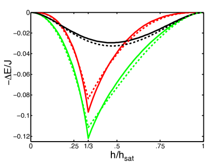
Figure 6: (Color online) Energy differences between various states using the leading $1/S$ result from spin-wave theory (solid lines) and the biquadratic classical approximation (dashed lines). Green lines represent the difference between Y/UUD/V and inverted Y energies; red between Y/UUD/V and umbrella; and black between inverted Y and umbrella.

The full benefit of approximating quantum zero-point energy by the classical biquadratic interaction will become clear when we address the effects of spatial anisotropy $J^{\prime}\neq J$ in Secs. VI.2 and VII.2. The classical energy gain due to spatial anisotropy is quadratic in the difference $J-J^{\prime}$. Such second-order corrections are not in general easy to account for analytically, making it difficult to consistently compare the anisotropy-induced energy splittings with those arising from quantum effects and DM interactions. Using the biquadratic interaction in Eq. (13), however, allows us to circumvent this problem and find the result of the competition between the different perturbations by numerically studying, via standard Monte Carlo techniques, the classical system described by $H_{0}+H_{\rm DM}+\delta H_{\rm bi}$. Later we will refer to ground states obtained within such a classical model with biquadratic spin couplings as ‘pseudo-quantum ground states’ to emphasize that despite corresponding to classical spins, such states are expected to semi-quantitatively reflect the influence of quantum fluctuations.

As a warm-up exercise of such a strategy, we first simulate a simpler “isotropic plus biquadratic” Hamiltonian $H_{\rm iso+bi}=H_{0}+\delta H_{\rm bi}$. Figure 7 shows $dM/dh$ and the coplanarity $K$ for this model at a low temperature of $T=0.027J$. This low temperature was reached via simulated annealing to avoid becoming trapped in local (but not global) free-energy minima. Specifically, Monte Carlo simulations were performed on a $24\times 24$ system starting at $T=0.4J$, then cooling down in small $\Delta T=0.009J$ steps. At each temperature the system was equilibrated with $35,000$ Monte Carlo steps. Measurements were taken during the last 30,000 steps.

The pronounced minimum of $dM/dh$ visible in Fig. 7 over the field interval $2.2J\lesssim h\lesssim 3.2J$ identifies this region with the collinear UUD state. The coplanar nature of the adjacent phases is evident from the plot of $K$ vs. $h$ in the same Figure. Note that despite the very low temperature considered, a substantial UUD plateau remains whose width greatly exceeds that of the purely classical model without interactions; see Fig. 3 for comparison. The width of the plateau is in fact proportional to $\Delta(h)$ as discussed in Ref. Chubukov and Golosov, 1991: quantum fluctuations, modeled here by $\delta H_{\rm bi}$, produce a stable UUD magnetization plateau over a finite field interval, even at $T=0$. We note that the usual spin-wave approach predicts a plateau over a field interval of width $\Delta h\approx 1.8J/(2S)$, which is somewhat larger than the plateau width obtained in our isotropic-plus-biquadratic simulations.

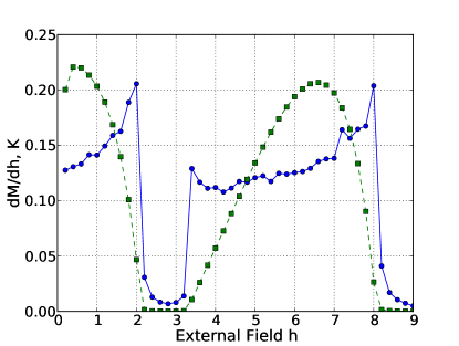
Figure 7: (Color online) $dM/dh$ (blue circles) and coplanarity $K$ (green squares), defined in Eq. (11), for the classical “isotropic plus biquadratic” model at $T=0.027J$, obtained by annealing from high temperature.

IV Spatially Isotropic Model with Dzyaloshinskii-Moriya Interactions: $J=J^{\prime},D\neq 0$

In this section we will explore how DM coupling affects the classical and quantum phase diagrams discussed above. One complication that arises here is that once we invoke DM interactions, the magnetic field direction is no longer arbitrary as it was in the previous section. Recall that the DM vector points along the $z$-axis. We will begin in Sec. IV.1 with the case where the field is applied along the $z$-direction, perpendicular to the triangular lattice plane. This field orientation is simplest to analyze since the Hamiltonian including $H_{DM}$ then preserves global U(1) spin symmetry about the $z$-axis. In-plane field orientations are studied in Sec. IV.2.

We should also emphasize that in any field orientation, DM coupling breaks $\pi/3$ rotation symmetry since $H_{\rm DM}$ in Eq. (2) only couples spins on neighboring ‘chains’ of the lattice. Thus the model with only DM coupling (and no spatial anisotropy) is clearly fine-tuned. Nevertheless, by examining the effects of DM alone we will gain valuable intuition that will be useful when we include the additional complication of spatial anisotropy in Sec. VII.

IV.1 Parallel orientation: ${\bf D}\parallel{\bf h}=h{\bf\hat{z}}$

IV.1.1 Classical Ground States

We will first explore how DM interactions lift the accidental degeneracy of the classical isotropic model using first-order perturbation theory. At this order, one simply needs to evaluate the DM energy using the unperturbed form of the classical ground states found in the previous section. Using the parametrization for the ground states in Eq. (6) and the constraints in Eqs. (7), we obtain

$$\langle H_{\rm DM}\rangle = 2\sigma ND\bigg{\{}-\sin^{2}\theta_{A}\sin^{2}\theta_{B}$$ (14)

$$+ \frac{1}{324J^{4}}[h^{2}+9J^{2}-6Jh(\cos\theta_{A}+\cos\theta_{B})$$

$$+ 18J^{2}\cos\theta_{A}\cos\theta_{B}]^{2}\bigg{\}}^{1/2},$$

where $\sigma={\rm sign}[\sin(\phi_{A}-\phi_{B})]$ determines the chirality of the spins in the $(x,y)$ plane. The DM energy above is minimized when $\cos\theta_{A}=\cos\theta_{B}=\frac{h}{9J}$ and $\sigma=-1$. One can readily see using Eqs. (7) that this corresponds to umbrella states of Fig. 2(f) for all fields (with a specific chirality because $D\neq 0$ breaks inversion symmetry). This outcome is quite natural given that DM coupling at ${\bf h}=0$ favors coplanar spiral order with spins pointing in the triangular lattice plane; the field simply cants the spiral out of the plane, producing an umbrella pattern. Note that this is markedly different from the coplanar and collinear configurations favored by thermal and quantum fluctuations. This leads to an interesting competition once one incorporates these additional ingredients, as we now address.

IV.1.2 Influence of thermal fluctuations

One can deduce the qualitative outcome of the competition between DM interactions and thermal fluctuations at finite temperature using the following general argument. In the previous section we discussed that while at $T=0$ the isotropic model exhibits many classically degenerate ground states, at finite temperature entropy lifts this degeneracy in favor of Y/UUD/V states. Moreover, this selection is strongest at intermediate temperatures where thermal fluctuations provide a large free-energy splitting but are not so severe as to destroy ordering altogether. (This can be seen most clearly through the width of the UUD plateau in Fig. 3, which reaches at maximum at around $T=0.35J$ before entering the paramagnetic phase at slightly higher $T$.)

Now suppose one slowly turns on DM interactions. At zero temperature any finite DM coupling will immediately select umbrella ordering since the entropic splittings vanish as $T\rightarrow 0$. By continuity umbrella states must persist over a finite temperature window that depends on both field and the DM coupling strength. Similarly, at intermediate temperatures the entropically favored Y/UUD/V states must also by continuity survive some amount of DM coupling. This leads to multi-stage ordering as a function of temperature. Consider for illustration the interesting example of one-third magnetization with weak DM coupling. As temperature increases from zero the system will begin in an umbrella state, transition into an UUD plateau at intermediate temperatures, and eventually give way to a paramagnet at high temperatures.

The qualitative picture that emerges is that as one increases DM coupling from zero, DM interactions eat away at the entropically-stabilized regions from the low-temperature side, eventually removing the Y/UUD/V phases entirely in favor of umbrella order at sufficiently large coupling. Obtaining a more quantitative understanding of this competition requires extensive Monte Carlo simulations, which we will not explore here. We will instead perform such a study in the more physically relevant case with spatial anisotropy in Sec. VI.1, where very similar physics arises. It should also be kept in mind that in this subsection we neglected quantum effects entirely. Below we incorporate quantum fluctuations and show that they lead to a substantially richer zero-temperature phase diagram than that of the purely classical model.

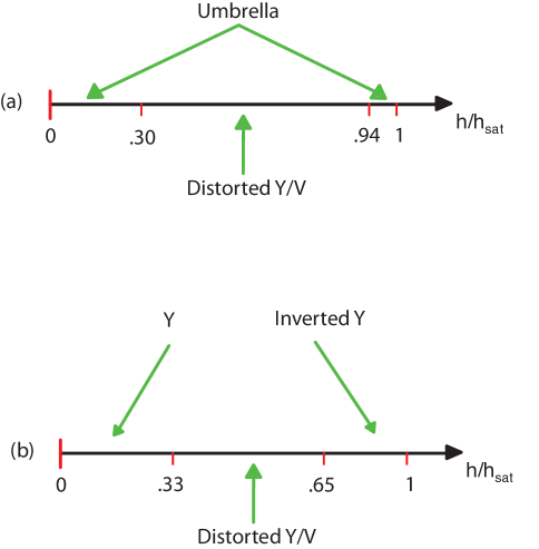
Figure 8: (Color online) Phase diagram of the quantum Heisenberg model with DM interactions, as a function of magnetic field $h$. The magnetic field orients along the DM axis, ${\bf D}\parallel{\bf h}$, in (a) and orthogonal to the DM axis, ${\bf D}\perp{\bf h}$, in (b).

IV.1.3 Quantum ground states

To incorporate DM interactions and quantum fluctuations at $T=0$, we treat $1/S$ and $D/J$ as expansion parameters of the same order of magnitude. The first-order corrections to the classical ground state energies can then be obtained simply by adding the $1/S$ spin-wave contribution discussed in Sec. III.4 to the classical DM energy in Eq. (14). [For example, the effect of quantum fluctuations on the DM energy produces a higher-order correction $\sim(D/J)(1/S)$.] By evaluating the perturbed energies for a dense subset of classical ground states as described in Sec. III.4, one can determine the spin order selected when both competing effects are present.

Carrying out this procedure with $D/J=0.05$ and $S=1/2$, we have found that the umbrella phase is the quantum ground state for sufficiently small magnetization ($h/h_{\rm sat}\lesssim 0.3$) and, also, sufficiently near saturation ($h/h_{\rm sat}\gtrsim 0.94$); see Fig. 8(a) which summarizes our numerics for this case. In between, however, a different ground state emerges which reflects a compromise between DM interactions and quantum fluctuations—the distorted V phase of Fig. 2(d). This state resembles the Y and V orders favored by quantum fluctuations, but is distorted in a non-coplanar fashion to gain DM energy. Note that the distortion of the spins away from perfect Y or V order is not unexpected: these states, as well as UUD, exhibit rotation symmetry which is explicitly broken by the DM interaction in Eq. (2) (recall the discussion at the end of Sec. III.2). The analytical structure of the distorted V state is easy to obtain in the high magnetic field limit as described in Sec. V.2.

IV.2 Orthogonal orientation: ${\bf D}\perp{\bf h}=h{\bf\hat{x}}$

IV.2.1 Classical Ground States

We will now extend the analysis of the previous section to the case where the magnetic field is applied in the plane of the triangular layers, along the $x$-direction for concreteness. This field orientation is complicated by the fact that the quantum Hamiltonian including DM coupling now lacks U(1) spin symmetry; instead the Hamiltonian is symmetric only under discrete spin rotations $S^{x}_{\bf r}\rightarrow S^{x}_{-{\bf r}}$ and $S^{y,z}_{\bf r}\rightarrow-S^{y,z}_{-{\bf r}}$. As above, we start by deducing the order favored by DM coupling in this field orientation using first-order perturbation theory. Using Eq. (6) to parametrize the classical ground states along with the constraints in Eqs. (7), the first-order correction to the energy arising from DM coupling can be written

$$\langle H_{\rm DM}\rangle = -\frac{2DN}{9J}[h(\sin\theta_{B}\sin\phi_{B}-\sin\theta_{A}\sin\phi_{A})$$ (15)

$$+ 9J\sin\theta_{A}\sin\theta_{B}\sin(\phi_{A}-\phi_{B})],$$

where the angles are subject to the additional constraint

$$\frac{1}{2}\left[1+\left(\frac{h}{3J}\right)^{2}\right] = \frac{h}{3J}(\sin\theta_{A}\cos\phi_{A}+\sin\theta_{B}\cos\phi_{B})$$ (16)

$$- \sin\theta_{A}\sin\theta_{B}\cos(\phi_{A}-\phi_{B})$$

$$- \cos\theta_{A}\cos\theta_{B}.$$

One can use Eq. (16) to eliminate $\theta_{B}$ from Eq. (15) and then minimize the DM energy over the remaining angles $\theta_{A},\phi_{A}$, and $\phi_{B}$. In this way we find that DM coupling selects coplanar inverted-Y states of Fig. 2(e), with

$$\theta_{A/B/C} = \pi/2$$

$$\phi_{A} = -\phi_{B}=\cos^{-1}\left[\frac{1}{2}\left(\frac{h}{3J}-1\right)\right]$$ (17)

$$\phi_{C} = 0.$$

The emergence of planar ground states for this field orientation is quite natural, again because DM interactions favor spins orienting within the triangular lattice plane. Among the various planar arrangements, inverted-Y states most effectively gain DM energy by keeping neighboring spins as far from parallel as possible (within the constraints set by the ground state manifold). In contrast, the UUD and V states favored by quantum fluctuations yield a vanishing first-order DM energy because in both configurations spins on two sublattices are parallel. We note that the favorability of inverted-Y over Y states at low fields is less obvious; the latter also gains DM energy, though to a lesser extent than the former.

Just as in the ${\bf h}=h{\bf\hat{z}}$ field orientation, incorporating thermal or quantum fluctuations therefore leads to a delicate competition with DM interactions. The discussion from Sec. IV.1.2 regarding entropic effects applies in this field orientation as well. Perhaps the most important qualitative distinction with the ${\bf h}=h{\bf\hat{z}}$ field orientation is the additional loss of U(1) symmetry here due to the orthogonality between ${\bf h}$ and ${\bf D}$ vectors. This implies the demise of the 1/3 magnetization plateau since the UUD and Y states then no longer constitute distinct phases separated by a spontaneous U(1) symmetry breaking. Sec. VII.2 discusses this effect in greater detail; see Fig. 15 for an illustration of the rounding-off of the magnetization plateau by DM interactions.

In the following subsection we will resolve the outcome of the competition between quantum fluctuations and DM interactions at zero temperature, which is qualitatively different from the previously considered ${\bf h}=h{\bf\hat{z}}$ case.

IV.2.2 Quantum Ground States

The quantum zero-temperature phase diagram in this field orientation is obtained as described in Sec. IV.1.3, again treating quantum corrections and DM coupling to first order with $D/J=0.05$ and $S$ extrapolated to $1/2$. Figure 8(b) depicts our results. Quantum effects and DM coupling compete in a subtle manner for this field orientation. The former dominates at low fields, where Y states prevail, while the latter dominates at high fields where inverted-Y states appear. Distorted V order, which reflects a nontrivial compromise between the two competing effects, appears at intermediate magnetization, $1/3\lesssim h/h_{\rm sat}\lesssim 0.65$. Note that all states are either perfectly planar or very nearly so here, which again is rather natural. Also notable is the absence of the collinear UUD state in the quantum phase diagram. As argued above, this is caused by the loss of U(1) spin symmetry in the ${\bf D}\perp{\bf h}$ geometry.

Observe that the quantum phase diagrams predicted for the two field orientations, ${\bf h}\propto{\bf\hat{z}}$ and ${\bf h}\propto{\bf\hat{x}}$, are very different. At either low or high fields, this implies that at least one phase transition separating the umbrella and Y/inverted-Y states ought to appear as one rotates the field from the $z$-direction to the $x$-direction. Recent experimentsTakano (2011) do indeed find a very complicated evolution of the phase diagram as the field rotates in this plane, featuring several intervening phase transitions. Generalizing the results of this paper to explore this crossover would be an interesting future research direction.

V BEC analysis near saturation

We will now shift our focus to phases realized at high magnetic fields near saturation, which can be elegantly described via Bose-Einstein condensation of magnon excitations above the fully polarized (saturated) state Batyev and Braginskii (1984); Nikuni and Shiba (1995); Veillette et al. (2005); Giamarchi et al. (2008); Ueda and Totsuka (2009). In this way magnetically ordered phases just below saturation $(h=h_{\rm sat}-\delta h)$ can be understood as a BEC instability of the ground state just above saturation $(h=h_{\rm sat}+\delta h)$. This limit has the advantage of allowing one to incorporate all of the competing effects of interest—quantum fluctuations, DM coupling, and spatial anisotropy—in a single controlled and coherent framework.

V.1 Preliminaries: $J=J^{\prime},D=0$

At $h>h_{\rm sat}$ the ground state of the Heisenberg Hamiltonian is known exactly: it is given by the fully polarized eigenstate of the Hamiltonian in which all spins point ‘up’. The excitations are magnons, i.e., plane-wave states of overturned spins. These are conveniently described by Holstein-Primakoff bosons, similar to Eqs. (12). Since all spins point in the same direction, it suffices to consider only a single boson species here; thus we write

$$S^{z}({\bf r})=S-a^{\dagger}({\bf r})a({\bf r}),~{}S^{+}({\bf r})=\sqrt{2S}~{}a({\bf r}),$$ (18)

for all ${\bf r}$. The isotropic Heisenberg Hamiltonian without DM coupling then reads, neglecting $1/S$ and smaller contributions,

$$H = H_{0}+V$$

$$H_{0} = \sum_{\bf k}S[J({\bf k})-J({\bf Q})-\mu]a^{\dagger}_{\bf k}a_{\bf k}$$

$$V = \frac{1}{4N}\sum_{\bf k,k^{\prime},q}[2J({\bf q})-J({\bf k})-J({\bf k^{\prime}}-{\bf q})]$$ (19)

$$\times a^{\dagger}_{\bf k+q}a^{\dagger}_{\bf k^{\prime}-q}a_{\bf k^{\prime}}a_{\bf k}.$$

Here

$$J({\bf k}) = \sum_{j=1}^{3}J_{{\bf r},{\bf r}+{\bm{\delta}}_{j}}\cos({\bf k}\cdot{\bm{\delta}}_{j})$$ (20)

$$= J\left[\cos(k_{x})+2\cos(k_{x}/2)\cos(\sqrt{3}k_{y}/2)\right]$$

is the Fourier transform of the exchange interaction, and

$$\mu=(h_{\rm sat}-h)/S$$ (21)

is the chemical potential which controls the state of the bosonic system. For $h>h_{\rm sat}$ the chemical potential is negative and the ground state is the boson vacuum $|0\rangle$ satisfying $a_{\bf k}|0\rangle=0$ for all ${\bf k}$. The wavevector ${\bf Q}$ in Eqs. (19) corresponds to the minimum of the magnon energy and follows from $J({\bf Q})=\text{min}_{\bf k}[J({\bf k})]$. A peculiarity of the triangular antiferromagnet Nikuni and Shiba (1995), and indeed many other frustrated spin systems Ueda and Totsuka (2009), is the fact that there are two distinct wavevectors minimizing $J({\bf k})$. For the isotropic two-dimensional triangular antiferromagnet these are $\pm{\bf Q}=(\pm 4\pi/3,0)$. Hence, at $h=h_{\rm sat}$ (or equivalently $\mu=0$), the magnon dispersion touches zero simultaneously at $\pm{\bf Q}$. One then needs to understand whether it is energetically favorable to condense magnons at one or both of these wavevectors, i.e., form a single-$Q$ or double-$Q$ condensate.

The analysis proceeds by parametrizing the magnon modes as follows,

$$a_{\bf k}=\sqrt{N}\psi_{+Q}\delta_{{\bf k},{\bf Q}}+\sqrt{N}\psi_{-Q}\delta_{{\bf k},-{\bf Q}}+\tilde{a}_{\bf k}.$$ (22)

Here $\tilde{a}_{\bf k}$ describes non-condensed magnons with ${\bf k}\neq\pm{\bf Q}$. The leading contribution to the energy (per site) is obtained by neglecting the non-condensed particles altogether. Written in terms of condensate densities $\rho_{1,2}=|\psi_{\pm Q}|^{2}$, the energy reads

$$\frac{E}{N}=-S\mu(\rho_{1}+\rho_{2})+\frac{1}{2}\Gamma_{1}(\rho_{1}^{2}+\rho_{2}^{2})+\Gamma_{2}\rho_{1}\rho_{2}.$$ (23)

The coefficients $\Gamma_{1,2}$ will be defined momentarily below, but first it is useful to discuss the important physics described by this simple equation in some generality. When $\mu<0$, the energy is minimized by a vacuum state with no condensate, $\rho_{1,2}=0$. Increasing $\mu$ (by lowering $h$) to positive values leads to a condensed state. A double-$Q$ condensate emerges for $\Gamma_{1}>\Gamma_{2}$, when $\rho_{1}=\rho_{2}=S\mu/(\Gamma_{1}+\Gamma_{2})$. The physical meaning of this is found by expressing the spin operators in terms of boson condensates. Using $\psi_{\pm Q}=\sqrt{\rho_{1}}e^{i\theta_{1,2}}$ and writing $\theta_{1,2}=\theta_{+}\pm\theta_{-}$, we find

$$S^{+}_{\bf r} = 2S\sqrt{\frac{2\mu}{\Gamma_{1}+\Gamma_{2}}}e^{i\theta_{+}}\cos[{\bf Q}\cdot{\bf r}+\theta_{-}],$$

$$S^{z}_{\bf r} = S-\frac{8\mu S}{\Gamma_{1}+\Gamma_{2}}\cos^{2}[{\bf Q}\cdot{\bf r}+\theta_{-}].$$ (24)

Hence, the double-$Q$ condensate describes a coplanar magnetically ordered state. Observe that the $S^{z}$ spin component is modulated with wavevector $2{\bf Q}$. The coplanar state described by Eq. (24) thus represents a ‘supersolid’ phase of the magnet. A single-$Q$ condensate arises when $\Gamma_{1}<\Gamma_{2}$; in this case $\rho_{1}=S\mu/\Gamma_{1}$ and $\rho_{2}=0$ or vice versa. This state corresponds to a conventional umbrella (or cone) magnetic structure:

$$S^{+}_{\bf r} = S\sqrt{\frac{2\mu}{\Gamma_{1}}}\exp[i{\bf Q}\cdot{\bf r}+i\theta_{1}],$$

$$S^{z}_{\bf r} = S-\frac{\mu S}{\Gamma_{1}}.$$ (25)

The classical (order $1/S^{0}$) expression for $\Gamma_{1,2}$ is given by

$$\Gamma_{1}=J(0)-J({\bf Q}),~{}\Gamma_{2}=J(0)-2J({\bf Q})+J(2{\bf Q}).$$ (26)

The accidental degeneracy of the classical isotropic triangular antiferromagnet discussed in Sec. III.1 manifests itself via the relation $\Gamma_{1}-\Gamma_{2}=J({\bf Q})-J(2{\bf Q})=0$ for ${\bf Q}=(4\pi/3,0)$. Thus the coplanar and cone states are degenerate classically. At first order in $1/S$ one finds

$$\Gamma_{1}>\Gamma_{2}$$ (27)

so that quantum fluctuations select coplanar state, consistent with our earlier spin-wave analysis. The corresponding calculation is sketched in Refs. Nikuni and Shiba, 1995; Ueda and Totsuka, 2009 and will not be discussed here for brevity. Instead, here we take Eq. (26) as given and ask how the addition of weak DM interaction in Eq. (2) as well as spatial anisotropy influences the delicate balance between coplanar and umbrella states at high magnetic fields.

V.2 Spatially Isotropic Model with Dzyaloshinskii-Moriya Interactions: $J=J^{\prime},D\neq 0,{\bf h}=h{\bf\hat{z}}$

In the geometry with ${\bf h}=h{\bf\hat{z}}$ the DM Hamiltonian in Eq. (2) reduces to a simple quadratic form of magnon operators,

$$H_{\rm{DM}} = \frac{iD}{2}\sum_{{\bf r},j=1,3}\Big{(}S^{-}_{\bf r}S^{+}_{{\bf r}+{\bm{\delta}}_{j}}-\text{h.c.}\Big{)}$$

$$= iDS\sum_{{\bf r},j=1,3}\Big{(}a^{\dagger}_{\bf r}a_{{\bf r}+{\bm{\delta}}_{j}}-\text{h.c.}\Big{)}$$

$$= -2NDS[\sin({\bf Q}\cdot{\bm{\delta}}_{1})+\sin({\bf Q}\cdot{\bm{\delta}}_{3})](\rho_{1}-\rho_{2}).$$

As expected physically, DM coupling breaks the symmetry between $\pm{\bf Q}$ points, and lowers the energy of the $\psi_{+Q}$ condensate (for positive $D>0$). The ground state follows from minimizing

$$\frac{E}{N} = -S\mu(\rho_{1}+\rho_{2})-Sg(\rho_{1}-\rho_{2})+$$ (29)

$$+\frac{1}{2}\Gamma_{1}(\rho_{1}^{2}+\rho_{2}^{2})+\Gamma_{2}\rho_{1}\rho_{2},$$

where we introduced $g=2\sqrt{3}D>0$. Following Ref. Bruce and Aharony, 1975, we parameterize the densities as

$$\rho_{1} = \rho\cos^{2}\phi$$

$$\rho_{2} = \rho\sin^{2}\phi$$ (30)

and minimize the energy with respect to $\phi$ and $\rho$.

Three possible solutions exist:

$$(\text{i})~{}\phi=0,\rho=\frac{S(\mu+g)}{\Gamma_{1}},\frac{E}{N}=-\frac{S^{2}(\mu+g)^{2}}{2\Gamma_{1}}$$ (31)

$$(\text{ii})~{}\phi=\frac{\pi}{2},\rho=\frac{S(\mu-g)}{\Gamma_{1}},\frac{E}{N}=-\frac{S^{2}(\mu-g)^{2}}{2\Gamma_{1}}$$ (32)

$$(\text{iii})\cos^{2}\phi=\frac{1}{2}\left[1+\frac{g(\Gamma_{1}+\Gamma_{2})}{\mu(\Gamma_{1}-\Gamma_{2})}\right],\rho=\frac{2\mu S}{\Gamma_{1}+\Gamma_{2}},$$

$$~{}~{}~{}~{}~{}~{}~{}~{}~{}\frac{E}{N}=-\frac{\mu^{2}S^{2}}{\Gamma_{1}+\Gamma_{2}}-\frac{g^{2}S^{2}}{\Gamma_{1}-\Gamma_{2}}.$$ (33)

Solutions (i) and (ii) describe umbrella states formed from a single-$Q$ condensate. For positive $g$ the umbrella corresponding to (i) with $\rho_{1}\neq 0,\rho_{2}=0$ has lower energy. The ‘mixed’ solution (iii), which only exists when $-1\leq g(\Gamma_{1}+\Gamma_{2})/\mu(\Gamma_{1}-\Gamma_{2})\leq 1$, yields the lowest energy provided that Eq. (27) is satisfied. This solution represents the distorted V state of Fig. 2(d), discussed in Sec. IV.1.3 above. The condensates here satisfy

$$|\psi_{+Q}|^{2} = \frac{\mu S}{\Gamma_{1}+\Gamma_{2}}+\frac{gS}{\Gamma_{1}-\Gamma_{2}},$$

$$|\psi_{-Q}|^{2} = \frac{\mu S}{\Gamma_{1}+\Gamma_{2}}-\frac{gS}{\Gamma_{1}-\Gamma_{2}},$$ (34)

and, as a result, the spin structure is non-coplanar,

$$S^{+}_{\bf r} = \sqrt{2S}e^{i\theta_{+}}\Big{[}(|\psi_{+Q}|+|\psi_{-Q}|)\cos({\bf Q}\cdot{\bf r}+\theta_{-})$$ (35)

$$+i(|\psi_{+Q}|-|\psi_{-Q}|)\sin({\bf Q}\cdot{\bf r}+\theta_{-})\Big{]}.$$

The degree of non-coplanarity is controlled by the DM coupling $g$. The distorted V state has finite longitudinal chirality [recall Eq. (8)] which is proportional to the density imbalance between the $\pm{\bf Q}$ condensates,

$$\kappa_{z}\sim 2S(|\psi_{+Q}|^{2}-|\psi_{-Q}|^{2}).$$ (36)

Thus, when the magnetic field orients along the DM vector, the transition from the fully polarized state proceeds in two steps as summarized in the schematic phase diagram of Fig. 9. Initially, at $\mu=-g$, one enters the umbrella state with ordering wavevector ${\bf Q}$. This state persists at lower fields until $\mu=g(\Gamma_{1}+\Gamma_{2})/(\Gamma_{1}-\Gamma_{2})$, where it is replaced by a distorted V state with condensates at both $\pm{\bf Q}$ wavevectors. These findings agree fully with a very different analysis in Sec. IV.1, which was carried out for specific values of $D/J$ and $1/S$. Our results here show that the two phases obtained at high fields near saturation in fact emerge very generally provided DM coupling is weak and quantum fluctuations can be adequately captured perturbatively.

Figure 9: (Color online) Phase diagram of the model in Eq. (29). The fully polarized state corresponds to $\rho=0$, while all other states exhibit a finite boson density, $\rho>0$. Umbrella states correspond to $\phi=0$ and $\pi/2$, while the mixed state with $0<\phi<\pi/2$ represents a distorted V phase. Observe that the origin of the phase diagram represents a tetracritical point.

V.3 Spatially Isotropic Model with Dzyaloshinskii-Moriya Interactions: $J=J^{\prime},D\neq 0,{\bf h}=h{\bf\hat{x}}$

To apply the formalism developed in this section to the case where the field orients perpendicular to the DM vector, it is simplest to rotate ${\bf D}$ and ${\bf h}$ such that ${\bf h}=h{\bf\hat{z}}$ and ${\bf D}=D{\bf\hat{x}}$. The DM Hamiltonian then reduces to the following combination of three magnon operators,

$$H_{\rm{DM}} = D\frac{\sqrt{2S}}{2i}\sum_{{\bf r},j=1,3}\Big{[}(a_{\bf r}-a^{\dagger}_{\bf r})a^{\dagger}_{{\bf r}+{\bm{\delta}}_{j}}a_{{\bf r}+{\bm{\delta}}_{j}}$$ (37)

$$- a^{\dagger}_{\bf r}a_{\bf r}(a_{{\bf r}+{\bm{\delta}}_{j}}-a^{\dagger}_{{\bf r}+{\bm{\delta}}_{j}})\Big{]}.$$

Focusing on the condensates this expression reduces to

$$H_{\rm{DM}} = D\frac{\sqrt{2S}}{2i}\sum_{{\bf r},j=1,3}\Big{[}\psi^{*}_{+Q}\psi_{-Q}(\psi_{-Q}-\psi^{*}_{+Q})e^{-i3{\bf Q}\cdot{\bf r}}$$ (38)

$$\times [e^{-i2{\bf Q}\cdot{\bm{\delta}}_{j}}-e^{-i{\bf Q}\cdot{\bm{\delta}}_{j}}]+\{{\bf Q}\to-{\bf Q}\}\Big{]}.$$

At this point, commensurability of the three-sublattice spin structure acquires crucial importance, since this implies $e^{\pm i3{\bf Q}\cdot{\bf r}}=e^{\pm i4\pi x}=1$ for all sites ${\bf r}$ of the triangular lattice. The end result, obtained by separating the magnitudes and phases of the condensates using Eqs. (30), is rather compact:

$$H_{\rm{DM}}=N4\sqrt{6S}D\rho^{3/2}\sin\theta_{+}\sin(3\theta_{-}).$$ (39)

Notice that Eq. (39) is independent of $\phi$. This angle is then determined solely by quantum effects which select coplanar order, the detailed structure of which is set by the angles $\theta_{\pm}$. In principle, quantum fluctuations do distinguish the latter angles and favor V ordering near saturation; this selection is, however, very weak and appears only when one includes higher-order terms in Eq. (23) (involving six boson fields)Nikuni and Shiba (1995). In contrast DM coupling distinguishes these angles more readily. One can immediately observe that, for $D>0$, minimization of Eq. (39) requires that $\theta_{+}=\pm\pi/2$. Let us choose for concreteness $\theta_{+}=+\pi/2$. By consulting Eq. (24), one finds that the plane in which spins order is orthogonal to the (rotated) DM vector. That is,

$$S^{x}_{\bf r} = 0$$

$$S^{y}_{\bf r} = \sqrt{8S\rho}\cos({\bf Q}\cdot{\bf r}+\theta_{-}).$$ (40)

At the same time, we need to impose $\sin(3\theta_{-})=-1$ given our choice for $\theta_{+}$. The different solutions for $\theta_{-}$ simply describe equivalent magnetic structures connected by lattice translations, so we focus for concreteness on $\theta_{-}=\pi/2$. This choice results in $S^{y}_{\bf r}=-\sqrt{8S\rho}\sin({\bf Q}\cdot{\bf r})$. For the triangular lattice the product

$${\bf Q}\cdot{\bf r}=\frac{2\pi}{3}\nu~{}\text{mod}~{}2\pi$$ (41)

takes on three inequivalent values: $0$ ($\nu=0$), $2\pi/3$ ($\nu=1$), and $-2\pi/3$ ($\nu=-1$). Correspondingly, the ordered $S^{y}$ spin components take on values which are zero ($\nu=0$), positive ($\nu=1$) and negative ($\nu=-1$). This represents the three-sublattice inverted-Y state found previously in Section IV.2 for a specific value of $D/J$ and $1/S$. The rather different approach adopted here reveals that the onset of inverted Y order induced by DM coupling near saturation is in fact a very generic conclusion.

V.4 Interplay Between Spatial Anisotropy and Dzyaloshinskii-Moriya Interactions: $J\neq J^{\prime},D\neq 0$

We will now begin addressing for the first time the influence of spatial anisotropy, which can be incorporated in a particularly simple manner near the saturation field. Let us first address the classical model without DM coupling. When $J\neq J^{\prime}$ the Fourier transform of the exchange interaction in Eq. (20) is now minimized at generally incommensurate wavevectors $\pm{\bf Q}$ given by

$${\bf Q}=2\cos^{-1}{\left(\frac{-J^{\prime}}{2J}\right)}{\bf\hat{x}}.$$ (42)

Consequently the difference between $\Gamma_{1,2}$ defined in Eqs. (26) is non-zero already at the classical level; to order $(J-J^{\prime})^{2}/J^{2}$, one finds $\Gamma_{1}-\Gamma_{2}=-9(J-J^{\prime})^{2}/(2J)$. It follows from our analysis in Sec. V.1 that since $\Gamma_{2}>\Gamma_{1}$ here, incommensurate umbrella states are stabilized classically below the saturation field, even with arbitrarily weak exchange anisotropy.

The inclusion of quantum fluctuations changes the situation in an interesting way. Recalling that $\Gamma_{1}>\Gamma_{2}$ due quantum effects in the isotropic limit, to leading order in $1/S$ and second order in exchange anisotropy we have

$$\Gamma_{1}-\Gamma_{2}\approx\frac{\alpha J}{S}-\frac{9(J-J^{\prime})^{2}}{2J}$$ (43)

for some constant $\alpha$. It is now apparent that the planar ordering favored by quantum fluctuations is in fact stable over a finite range of anisotropy, though due to the shift in ${\bf Q}$ such planar configurations will now be incommensurate. Only when the anisotropy reaches a critical strength are these states supplanted by umbrella order.

This analysis can be readily extended to incorporate DM coupling as well. Consider first the field orientation ${\bf h}=h{\bf\hat{z}}$, where the magnetic field and ${\bf D}$ vector are parallel. As long as spatial anisotropy is sufficiently weak that $\Gamma_{1}$ exceeds $\Gamma_{2}$, the phase diagram shown in Fig. 9 remains qualitatively intact (though the umbrella and distorted V states become incommensurate). As $|J-J^{\prime}|$ increases, the incommensurate distorted V state arises over a progressively smaller region of the phase diagram until, when $\Gamma_{1}=\Gamma_{2}$, it is removed entirely. At larger anisotropy only incommensurate umbrella phases appear just below saturation.

The case where the magnetic field orients perpendicular to the DM vector is even more straightforward. In the preceding subsection the effectiveness of DM coupling relied critically on the wavevector ${\bf Q}$ being commensurate; see Eq. (38). With incommensurate ${\bf Q}$ the corresponding term sums to zero and thus drops out. Thus the DM interaction is effectively gone and we then recover the physics discussed above for the anisotropic quantum model without DM interactions.

VI Spatially Anisotropic Model: $J\neq J^{\prime},D=0$

VI.1 Classical limit

In the remaining sections we will endeavor to address the phase diagram in the presence of spatial anisotropy at arbitrary fields. We start by treating the case without DM interactions for simplicity. Arbitrarily weak anisotropy $J-J^{\prime}$ destroys the accidental classical ground state degeneracy of the isotropic model in favor of an incommensurate spiral ground state at all fields, similarly to the situation described above near saturation. The ordering wavevector is in fact given by Eq. (42) for all values of the magnetic field below saturation; the corresponding spin state is described by

$${\bf S}({\bf r})=\sin{\theta}\left[\cos{\left({\bf Q}\cdot{\bf r}\right)}{\bf\hat{x}}+\sin{\left({\bf Q}\cdot{\bf r}\right)}{\bf\hat{y}}\right]+\cos\theta{\bf\hat{z}}.$$ (44)

While a unique classical ground state therefore emerges for all fields at zero temperature, the finite-temperature phase diagram is much more complicated and interesting. This can be anticipated on physical grounds. Indeed, as a general rule thermal fluctuations prefer coplanar over non-coplanar states (see the discussion in Sec. III); thus for sufficiently weak anisotropy one can expect that the entropic gain from planar order should be able to overcome its classical energy cost over a range of temperatures. This means that planar states should appear above some critical temperature $T_{\rm pl}$. It is reasonable to expect that $T_{\rm pl}\sim(J-J^{\prime})^{2}/J$ since the classical energy gain by umbrella states occurs at second order in $J-J^{\prime}$. It is also clear that as $J-J^{\prime}$ increases, the planar states will be gradually pushed towards higher temperatures and disappear altogether above some critical value (which is magnetic-field dependent) of the spatial anisotropy.

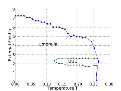
Figure 10: (Color online) Phase diagram of the classical anisotropic model with $J^{\prime}/J=0.765$. Interestingly, at this anisotropy strength the entropically favored planar phases are absent (within the resolution of our numerics), save for the collinear UUD state which now requires intermediate temperatures to appear.

Of all the planar phases considered the UUD state, which in fact is collinear, yields the highest entropy at finite temperature. The relative stability of the UUD state over the Y and V states is clear already at the spatially isotropic point: Figure 3 shows that at finite $T$ the collinear state expands at the ‘expense’ of the planar ones. We thus expect the UUD state to persist the most upon deformation of the model’s parameters. Our numerical findings fully support this conclusion and reveal the rather non-trivial phase structure of the classical model. Figure 10 displays the rough phase diagram obtained using classical Monte Carlo with $J^{\prime}/J=0.765$. This value was chosen due to its closeness to the estimate for Cs₂CuBr₄, and the fact that for this anisotropy strength the wavevector ${\bf Q}$ ‘fits’ into the $48\times 48$ system so that incommensurate orders are not frustrated in the geometries we simulated. In these simulations we have taken $20,000$ Monte Carlo steps for thermalization and $20,000$ more for measurements.

Remarkably, the UUD state indeed remains and ‘floats’ above the energetically preferred umbrella phase. The UUD order can be clearly identified by the behavior of $dM/dh$ versus field. As shown in Fig. 11, at an intermediate temperature of $T=0.168J$ we observe a pronounced dip in $dM/dh$, indicating a diminished slope of the magnetization in the field interval between $h_{c1}$ and $h_{c2}$. Of course slower growth of the magnetization is expected for the magnetization plateau. At a lower temperature of $T=0.12J$, $dM/dh$ shows no such variation indicating the absence of UUD order. This picture is further corroborated by the temperature dependence of the chirality as Fig. 12 illustrates for $h=2.3J$. One clearly sees a discontinuous jump at $T\approx 0.13J$ in both the transverse and longitudinal chiralities, indicating a first-order finite-temperature transition from the entropy-stabilized UUD state to an umbrella phase. Note that, with the possible exception of the small regions near the UUD boundary where our numerics do not have enough accuracy to reach any definite conclusions, the Y and V planar states are absent in the phase diagram. At the anisotropy we analyzed here they are replaced by the energetically favorable umbrella structure.

The already non-trivial phase diagram we obtained here certainly deserves more extensive numerical investigation. In particular it would be interesting to perform a systematic study increasing $J-J^{\prime}$ from zero to explore the collapse of the Y/UUD/V states and accompanying onset of umbrella order. We note that a similar finite-temperature competition between energetically-favorable and entropically-favorable states has been previously reported in more complex spin systems: frustrated pyrochlore Pinettes et al. (2002); Chern et al. (2008) and Shastry-Sutherland antiferromagnets Moliner et al. (2009). It is worth noting that the roots of this behavior can be traced to the famous “Pomeranchuk effect” in ³He where the crystal phase of ³He, which is characterized by exponentially weak in distance exchange interaction between localized spins, has higher entropy than the normal Fermi-liquid phase. As a result, upon heating the liquid phase freezes into a solidPomeranchuk (1950); Richardson (1997).

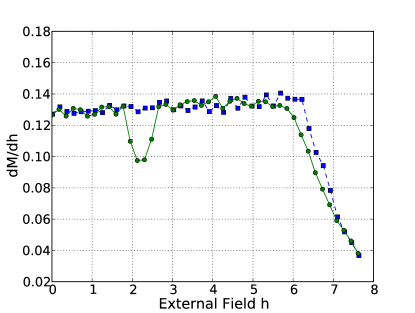
Figure 11: (Color online) $dM/dh$ versus $h$ at $T=0.168J$ (green circles) and $T=0.12J$ (blue squares) for the classical anisotropic model with $J^{\prime}/J=0.765$.

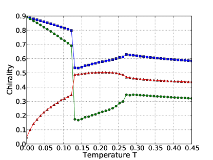
Figure 12: (Color online) Chiralities $\kappa$ (blue squares), $\kappa_{\perp}$ (red triangles) and $\kappa_{z}$ (green circles) versus $T$ at $h=2.3J$ for the classical anisotropic model with $J^{\prime}/J=0.765$. The discontinuous jumps near $T=0.13J$ signify a first-order transition between umbrella and UUD phases.

VI.2 Pseudo-quantum Ground States

Our goal now will be to use Monte Carlo numerics to understand the zero-temperature phase diagram when both exchange anisotropy and quantum effects (modeled via the biquadratic approximation discussed in Sec. III.5) are present. Again to avoid becoming trapped in a local energy minimum, the phase diagram was obtained using simulated annealing as described in Sec. III.5.

To explore the competition between anisotropy and quantum effects, simulations were performed with fixed $S=1/2$ but numerous anisotropies $J^{\prime}/J=1,0.95,0.9,0.85,0.8,0.765,0.7$. We used $M,dM/dh,K$ and $\bf{\kappa}$ to construct the phase diagram at each $J^{\prime}/J$; Fig. 13 summarizes our findings. An interesting feature of the phase diagram is the complete absence of non-coplanar umbrella states, despite the fact that this type of order uniquely minimizes the classical energy at all fields. Even for rather substantial anisotropy $J-J^{\prime}\sim 0.3J$, quantum effects (modeled here via the biquadratic interaction) qualitatively alter the magnetization process.

A second interesting feature is the persistence of commensurate Y/UUD/V states despite the exchange anisotropy. The UUD state is particularly stable, and at least within the approximations used is hardly affected by the finite $J-J^{\prime}$ values studied. In its vicinity commensurate Y and V states appear over a finite field interval, with the latter being more robust than the former against anisotropy. All of this is in agreement with the previous large-$S$ analytical investigation of Ref. Alicea et al., 2009. Incommensurate planar phases, which reflect a nontrivial compromise between quantum fluctuations and anisotropy, appear at low fields and near saturation; in the thermodynamic limit, these are expected to occupy a progressively larger portion of the phase diagram as anisotropy increases.

It is worth briefly remarking on finite-size effects in our simulations. First, in Fig. 13 the high-field incommensurate phase appears over a broader field range at $J^{\prime}/J=0.765$ than $J^{\prime}/J=0.7$. This artifact arises because the incommensurate spin structure that would appear in an infinite system is less frustrated by the periodic boundary conditions at the former anisotropy strength. Second, we note that incommensurate order sets in at low and high fields only when $J^{\prime}\lesssim 0.85J$ in our simulations. Closer to the isotropic limit, they are simply absent. This reflects finite-size effects arising from the relatively small systems modeled here. We expect that the phase boundary between the Y and incommensurate planar states emanates from the $h=0,J^{\prime}=J$ point. Similarly, the phase boundary between the V and the incommensurate planar states extends all the way to $h=h_{\rm sat},J^{\prime}=J$; indeed, in Sec. V.4 we found that arbitrarily weak anisotropy is sufficient to produce incommensurate planar order near saturation. These phase lines represent commensurate-incommensurate transitions. We have indicated the expected transitions with dashed lines in Fig. 13.

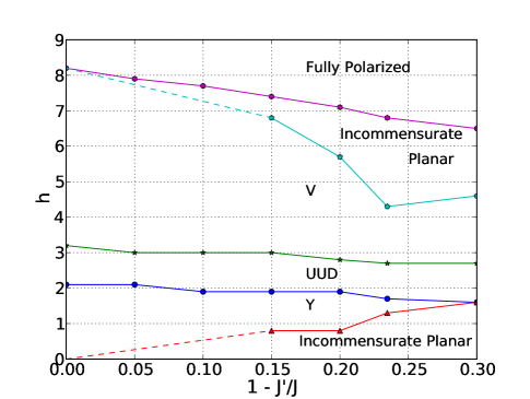
Figure 13: (Color online) Ground state phase diagram for the spatially anisotropic triangular antiferromagnet with quantum fluctuations modeled via the biquadratic approximation discussed in Sec. III.5. All data points were obtained with Monte Carlo simulated annealing numerics. Dashed lines represent phase boundaries which are absent due to finite-size effects in our simulations but are expected on general grounds for an infinite system.

VII Spatially Anisotropic Model with Dzyaloshinskii-Moriya Interactions: $J\neq J^{\prime},D\neq 0$

VII.1 Classical Ground States

Finally, we are in position to consider the full model featuring all of the ingredients we set out to study: spatial anisotropy, DM coupling, and quantum fluctuations. As a first step we will establish the phase diagram in the classical case. For fields ${\bf h}=h{\bf\hat{z}}$ directed along the DM vector the classical ground states simply correspond to incommensurate umbrella order for all fields up to saturation. This outcome is extremely natural given our earlier findings that for this field orientation both DM coupling and anisotropy separately favor umbrella states.

The phase diagram is more subtle for fields ${\bf h}=h{\bf\hat{x}}$ oriented perpendicular to the DM vector. We found earlier that spatial anisotropy favors incommensurate umbrella states, while DM interactions prefer inverted Y order; thus, the resolution of their competition is far from obvious. Focusing on $J^{\prime}/J=0.765$ (again, this value minimizes finite-size effects) and $D/J=0.05$, we find using simulated annealing that incommensurate coplanar order arises at low fields, $h\lesssim 0.34h_{\rm sat}$, reflecting a nontrivial compromise between these competing interactions. DM coupling dominates at intermediate fields $0.34h_{\rm sat}\lesssim h\lesssim 0.8h_{\rm sat}$, where inverted-Y states appear. The appearance of such a broad commensurate state in the anisotropic system even with only quadratic spin couplings is rather remarkable. Finally, at larger fields up to saturation spatial anisotropy dominates, leading to non-coplanar umbrella order. One can in fact analytically estimate the phase boundaries between these three spin states found in our numerics. The calculation is described in Appendix B, and the resulting classical phase diagram appears in Fig. 14.

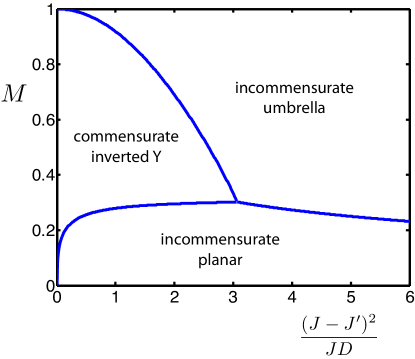
Figure 14: (Color online) Classical phase diagram for spins with spatially anisotropic exchange interactions, DM coupling, and a magnetic field applied perpendicular to the DM vector. Phase boundaries were computed analytically to leading order in DM strength $D/J$ and anisotropy strength $(J-J^{\prime})^{2}/J^{2}$ as described in Appendix B.

VII.2 Pseudo-quantum Ground States

Let us now explore how quantum effects—again modeled within the biquadratic approxiation—modify the classical phase diagrams discussed above. Consider first the ${\bf h}=h{\bf\hat{z}}$ field orientation. The situation at high fields was already analyzed in Sec. V.4, where we found the presence of umbrella order just below saturation, followed by an incommensurate planar state provided anisotropy was not too strong. At intermediate fields we found in the quantum problem with either DM coupling or spatial anisotropy that commensurate planar phases emerged. It is thus reasonable to anticipate the same outcome when both elements are present, at least for sufficiently weak DM coupling and anisotropy. At low fields DM coupling led to umbrella order in the quantum problem analyzed in Sec. IV.1.3, while the interplay between spatial anisotropy and quantum effects led to an incommensurate planar state in Sec. VI.2.

Putting together these findings suggests that the phase diagram for the spatially anisotropic pseudo-quantum model depicted in Fig. 13 evolves in the following manner as one increases the DM coupling strength from zero. First, umbrella order immediately begins to ‘eat away’ at the planar phases just below saturation, occupying a progressively larger fraction of the high-field phase diagram as the DM coupling increases. The low-field incommensurate planar state stabilized by the interplay between spatial anisotropy and quantum fluctuations is more robust against DM coupling. Only beyond a critical value of the DM coupling does umbrella order begin to take over in the low-field portion of the phase diagram. Of course more complicated scenarios are all possible, particularly if DM coupling and/or anisotropy are not especially weak; a detailed study of the problem for this field orientation would be interesting to carry out in future work.

Our main focus, however, is on the low-symmetry field orientation ${\bf h}=h{\bf\hat{x}}$ where the magnetic field and DM vectors are orthogonal. This is the physical situation relevant for the interesting experiments of Ref. Fortune et al., 2009 which motivated this study. We explored the zero-temperature phase diagram here using extensive simulating annealing numerics, modeling quantum fluctuations as before using the biquadratic approximation. We note that particular care must be taken when performing these simulations to avoid spurious finite-size effects. In particular, at low fields in $48\times 48$ systems we found an unusual incommensurate planar state exhibiting structure-factor peaks at two incommensurate wavevectors with non-zero momentum $Q_{y}$ along the $y$-direction. This phase, however, proved to arise due to finite-size effects—upon increasing the system size to $192\times 192$, order characterized by a single wavevector and vanishing $Q_{y}$ emerged.

Figure 16 summarizes our results. As noted in Sec. III.2, the Hamiltonian no longer possesses any continuous symmetries; hence some of the phase boundaries discussed earlier disappear from the phase diagram and become crossovers. One of these is the transition between the Y and the UUD states. The difference between these phases in the problem without DM coupling originates from the finite superfluid component of the Y state, present due to spontaneous breaking of U(1) spin rotations about the field axis, along with rotation symmetry which the Y state breaks but the UUD state does not. In the ${\bf D}\perp{\bf h}$ problem these two states are symmetry equivalent as they only break the same discrete lattice symmetries, and are thus not distinct phases. This shows up in our numerical simulations as a quick rounding of the lower end of the magnetization plateau upon increasing the DM coupling at fixed $J^{\prime}/J$, as illustrated in Fig. 15. Simultaneously, for $D$ as small as $D=0.01J$ the coplanarity $K$ becomes finite, although small, inside the former UUD interval between the Y and V states.

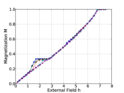
Figure 15: (Color online) Magnetization versus field at temperature $T=0.001J$ for the spatially anisotropic antiferromagnet with $J^{\prime}=0.765J$, DM interactions satisfying ${\bf D}\perp{\bf h}$, and quantum effects modeled via a biquadratic interaction. The curves shown correspond to different values of the DM strength: $D=0$ (blue circles), $D=0.01J$ (green triangles), $D=0.02J$ (red stars), $D=0.04J$ (cyan squares), and $D=0.05J$ (pink hexagons). The quick rounding of the lower edge of the plateau reflects the symmetry equivalence of the Y and UUD states when DM interactions are present in this field orientation.

We also observe persistence of the distorted V state at intermediate fields above the (former) UUD state. [Note that as discussed in Sec. III.2 the symmetry distinction between the distorted V and UUD orders persists in this field orientation, so that a bona fide phase transition separates these states.] In fact it appears that the distorted V state is the most stable of all the commensurate states considered previously. Because the spins in this phase can smoothly adjust to gain DM energy, this state survives even at the strongest DM coupling strength $D/J=0.05$ considered by us. By contrast, the previously robust UUD state, having lost its symmetry distinction from the less stable Y state as discussed above, is seen in Fig. 15 to essentially disappear for such a strong DM coupling.

Our simulations also reveal that for sufficiently strong DM coupling $D\gtrsim 0.04J$ a narrow region of the commensurate inverted Y state appears above the distorted V phase. This is quite consistent with the phase diagram of Fig. 14 for the classical model described in the previous subsection: being a prominent phase there, the inverted Y state is also natural in the quantum problem once quantum effects are sufficiently “weakened” by spatial anisotropy and DM interactions. The transition between the inverted Y and distorted V states appears continuous in our numerics and hard to pin down precisely, in part because the overall extent of this phase is rather narrow. For this reason its phase boundary in Figure 16 is less accurate than for the other phases.

The remaining high- and low-field regions are found to be occupied by the incommensurate coplanar states which owe their stability to quantum fluctuations. This is particularly clear for the high-field region near saturation where an incommensurate analog of the V state wins over the classical umbrella state only due to $1/S$ interactions between spin waves, as discussed in Sec. V.4.

Figure 16: Sketch of the phase diagram for the quantum spatially anisotropic model with varying DM coupling strength, $J^{\prime}/J=0.765$, and a magnetic field ${\bf h}$ oriented perpendicular to the DM vector. Data points indicate phase boundaries determined using simulating annealing numerics, with quantum fluctuations modeled via a biquadratic interaction. Dashed lines interpolate between these data points and are drawn for convenience. The location of the inverted Y phase is approximate as discussed in the main text.

VIII Conclusions

We have explored the phase diagram of a spatially anisotropic triangular lattice quantum antiferromagnet subject to asymmetric DM interactions and an external magnetic field. By treating spatial anisotropy $(J-J^{\prime})/J$, quantum fluctuations due to the finite spin value $S$, and DM coupling $D$ as perturbations of the well-understood isotropic classical antiferromagnet, we have found a rich variety of behaviors sensitive to the relative strengths of the perturbations considered. The root of this richness lies in the large accidental degeneracy of the unperturbed model with $J^{\prime}=J$, $S=\infty$ and $D=0$, along with the fact that each of these perturbations favors different ordered states in the manifold of accidentally degenerate configurations.

Our main findings are as follows:

1) In agreement with numerous previous studies, for the isotropic model without DM coupling we observe that quantum fluctuations select coplanar Y and V states and a collinear UUD phase out of infinitely many degenerate states available in the classical limit $S\rightarrow\infty$. Quantum effects most effectively split this degeneracy in the vicinity of one-third magnetization where nearly collinear low-energy states are accessible. This implies a greater robustness of the quantum-selected states to additional perturbations in these regions of the phase diagram, a trend that is indeed seen throughout our study. We also established that quantum effects can be semi-quantitatively modeled within a purely classical Hamiltonian by incorporating a biquadratic spin interaction with a field-dependent coupling chosen to mimic $1/S$ corrections to the classical ground state energies. Such a purely classical model has the virtue of allowing conventional Monte Carlo simulations to be employed to ascertain the (approximate) phase diagram when all the competing interactions of interest are present.

2) Adding DM interactions introduces two new commensurate states into consideration—distorted V and inverted Y orders. With fields applied perpendicular to the triangular lattice plane, DM coupling stabilizes umbrella order classically at all fields up to saturation. Quantum effects, however, stabilize a distorted V state at intermediate fields, bordered on both sides by the classically driven umbrella phase. For all in-plane fields up to saturation, DM interactions select inverted Y states classically. Quantum fluctuations are still more effective at modifying the phase diagram in this field orientation, producing Y order at low fields and a distorted V phase at intermediate fields. Only at high fields does the classically favored inverted Y state appear in the quantum problem. It is worth pointing out here that the new distorted V and inverted Y states also appear naturally in the theoretically simple limit of high magnetic fields near saturation, as discussed in Sec. V.

3) Spatial anisotropy, on the other hand, prefers non-coplanar umbrella (cone) configurations classically. Even this simple classical model, which has a unique ground state, harbors some surprises. We find that for sufficiently small spatial anisotropy an entropic order-by-disorder selection prevails over energetic considerations over a range of temperatures and magnetic fields. This results in an abrupt first-order phase transition from an umbrella state into a fluctuation-stabilized UUD state at finite temperature; see Sec. VI.1. This physically reasonable but so far unexplored feature of the classical Heisenberg model with anisotropic exchange interactions deserves more extensive numerical investigation on its own.

4) The competition between spatial anisotropy and quantum effects (simulated within an effective classical model with biquadratic spin couplings) results in a rich phase diagram shown in Fig. 13. These competing ingredients compromise to form incommensurate versions of the Y and V states at low and high fields, respectively. Remarkably, the intermediate-field region of the phase diagram in Fig. 13 is only weakly affected by the anisotropy strengths we analyzed, with the commensurate Y, UUD, and V states favored by quantum effects all appearing prominently. In particular, the UUD state which underlies the one-third-magnetization plateau, shows no obvious reduction in its width. All these features of the phase diagram agree well with previous analytical Alicea et al. (2009) and numerical Tay and Motrunich (2010) studies.

5) When spatial anisotropy, DM interactions, and quantum effects (again incorporated in an effective classical Hamiltonian) are all present, we obtain the phase diagram of Fig. 16, which contains most of the phases reviewed above. It is interesting to compare this with the experimental phase diagram of Ref. Fortune et al., 2009 which features up to nine different phases. Clearly our phase diagram is less diverse but still contains, for $D\approx 0.04J$, five different phases, most of which are coplanar. In particular it is tempting to speculate that one of the puzzling high-field phases (B, III, IV or 2/3, in the notation of Ref. Fortune et al., 2009) can be identified with the inverted Y state appearing near the phase boundary between the distorted V and the incommensurate planar phases. Further experiments that directly probe the spin structure in the various phases seen are, however, required to make a more definitive comparison with our results.

We emphasize here that nowhere in our study did we find hints of a possible two-thirds-magnetization plateau suggested by several experimental papers Ono et al. (2004, 2005); Fortune et al. (2009). In this regard the possibility of this novel magnetization plateau, at present identified theoretically only once Miyahara et al. (2006), requires more careful investigations. It must also be kept in mind that our treatment of quantum fluctuations is only perturbative, and certainly in the $S=1/2$ model at least the phase boundaries will be quantitatively different from what we have found. Whether or not strong quantum fluctuations can induce entirely new states, unseen in our semiclassical analysis, remains an interesting open question.

More broadly, our analysis relies on the observation that near the spatially isotropic point, where the relevant low-energy states form a three-sublattice pattern, the only relevant DM interaction is that given in Eq. (2). This implies that the phase diagram should be insensitive to the orientation of the magnetic field in the ${\bf b}-{\bf c}$ plane of the material. Recent experimental findings support this statement Takano (2011), and, in our view, should be interpreted as lending strong support to our perturbative approach to Cs₂CuBr₄. It is worth pointing out that this is certainly not the case for the isostructural material Cs₂CuCl₄; there it has been established experimentally that phase diagrams for the cases ${\bf h}\parallel{\bf b}$ and ${\bf h}\parallel{\bf c}$ are indeed different Tokiwa et al. (2006). That difference has been attributed to additional symmetry-allowed DM interactions Starykh et al. (2010) and, fundamentally, is tied to the fact that Cs₂CuCl₄ is very much a quasi-one-dimensional material, in contrast to Cs₂CuBr₄.

Another, and so far little explored, way to gain insight into the rich physics of frustrated antiferromagnets is provided by a magnetic system’s response to various impurities. Cs₂CuBr₄ has been probed in this way Ono et al. (2005), and initial theoretical investigations have appeared recently.Wollny et al. (2011)

We hope that our study will stimulate further theoretical and experimental studies of Cs₂CuBr₄, as well as related materials and models, in the near future.

Appendix A Symmetry-allowed Dzyaloshinskii-Moriya interactions in Cs₂CuBr₄

The general form of the DM interaction, consistent with crystal symmetry of Cs₂CuBr₄, was derived in Ref. Starykh et al., 2010 for the isostructural material Cs₂CuCl₄. For the three-dimensional crystal with layers indexed by $z$, it reads

$$H_{\rm{DM}} = \sum_{\bf r}({\bf D^{\prime}}\cdot{\bf S}_{\bf r}\times{\bf S}_{{\bf r}+{\bm{\delta}}_{2}}+{\bf D}^{+}\cdot{\bf S}_{\bf r}\times{\bf S}_{{\bf r}+{\bm{\delta}}_{1}}$$ (45)

$$- {\bf D}^{-}\cdot{\bf S}_{\bf r}\times{\bf S}_{{\bf r}-{\bm{\delta}}_{3}})$$

where

$${\bf D^{\prime}} = 2D_{z}(-1)^{z}{\bf\hat{z}}+D_{y}(-1)^{y}{\bf\hat{y}},$$ (46)

$${\bf D}^{\pm} = D_{z}^{\prime}(-1)^{z}{\bf\hat{z}}\pm D_{x}^{\prime}(-1)^{y+z}{\bf\hat{x}}+D_{y}^{\prime}(-1)^{y+z}{\bf\hat{y}}.$$ (47)

We are, however, interested in a 2D triangular antiferromagnet so will henceforth consider only one layer with $z=0$ for concreteness. We now show that for a weakly deformed triangular antiferromagnet, which is an appropriate characterization of Cs₂CuBr₄, only two DM couplings $D_{z}$ and $D_{z}^{\prime}$ need to be retained to leading order in perturbation theory. Furthermore, $D_{z}$ and $D_{z}^{\prime}$ yield first-order contributions which are in fact identical in nature and can thus be combined into a single DM coupling oriented along the crystal $z$-axis.

These results follow from the observation that all classical ground states of the isotropic model form a three-sublattice structure which repeats in the $y$-direction; see Fig. 1. Let us first consider the term $D_{y}$. Because of the repeating structure in the $y$-direction, we see that the cross products of spins from the A, B and C sublattices cancel out due to the oscillating $(-1)^{y}$ factor in the $D_{y}$ term. Thus $D_{y}$ can only appear at second-order or higher in perturbation theory, and for this reason can be neglected. Similar reasoning dictates that $D_{x}^{\prime}$ and $D_{y}^{\prime}$, which also include oscillating $(-1)^{y}$ factors, do not contribute to first order and can thus be omitted as well.

Consider now the remaining terms, $D_{z}$ and $D_{z}^{\prime}$. From Fig. 1 we see that ${\bf S}_{{\bf r}+{\bm{\delta}}_{1}}$ and ${\bf S}_{{\bf r}-{\bm{\delta}}_{2}}$ correspond to the same sublattice. Likewise, spins ${\bf S}_{{\bf r}+{\bm{\delta}}_{2}}$ and ${\bf S}_{{\bf r}-{\bm{\delta}}_{3}}$ can also be identified. Consequently, the most general DM Hamiltonian above, when evaluated in an arbitrary three-sublattice classical ground state, reduces to the following expression,

$$H_{\rm{DM}} \rightarrow \sum_{\bf r}{\bf\hat{z}}\cdot(2D_{z}{\bf S}_{\bf r}\times{\bf S}_{{\bf r}+{\bm{\delta}}_{2}}+D_{z}^{\prime}{\bf S}_{\bf r}\times{\bf S}_{{\bf r}+{\bm{\delta}}_{1}}$$ (48)

$$- D_{z}^{\prime}{\bf S}_{\bf r}\times{\bf S}_{{\bf r}-{\bm{\delta}}_{3}})$$

$$= \sum_{\bf r}{\bf\hat{z}}\cdot[(D_{z}{\bf S}_{\bf r}\times{\bf S}_{{\bf r}+{\bm{\delta}}_{2}}-D_{z}^{\prime}{\bf S}_{\bf r}\times{\bf S}_{{\bf r}-{\bm{\delta}}_{3}})$$

$$- (D_{z}{\bf S}_{{\bf r}}\times{\bf S}_{{\bf r}-{\bm{\delta}}_{2}}-D_{z}^{\prime}{\bf S}_{\bf r}\times{\bf S}_{{\bf r}+{\bm{\delta}}_{1}})]$$

$$\rightarrow (D_{z}-D_{z}^{\prime})\sum_{\bf r}{\bf\hat{z}}\cdot({\bf S}_{\bf r}\times{\bf S}_{{\bf r}-{\bm{\delta}}_{3}}-{\bf S}_{\bf r}\times{\bf S}_{{\bf r}+{\bm{\delta}}_{1}})$$

$$= (D_{z}^{\prime}-D_{z})\sum_{\bf r}{\bf\hat{z}}\cdot[{\bf S}_{\bf r}\times({\bf S}_{{\bf r}+{\bm{\delta}}_{1}}+{\bf S}_{{\bf r}+{\bm{\delta}}_{3}})].$$

Hence, defining ${\bf D}=(D_{z}-D_{z}^{\prime}){\bf\hat{z}}\equiv D{\bf\hat{z}}$, we arrive at the DM Hamiltonian in Eq. (2).

Appendix B Analytical determination of phase boundaries in Figure 14

In this Appendix we will sketch the derivation of the phase boundaries depicted in Fig. 14. We adopt a variational approach and calculate the energies for the three phases found in simulations—incommensurate planar, commensurate inverted-Y, and incommensurate umbrella states—to determine which minimizes the energy as a function of field. Of course there is no guarantee that only these three phases are relevant, but our numerical findings suggest that this is the case for weak anisotropy and DM coupling.

For concreteness, let us take the field in the $y$-direction. For the incommensurate planar state, we work at low fields and parametrize the spins as

$${\bf S}_{\bf r}=\cos[{\bf Q}\cdot{\bf r}+\phi({\bf r})]{\bf\hat{x}}+\sin[{\bf Q}\cdot{\bf r}+\phi({\bf r})]{\bf\hat{y}},$$ (49)

where ${\bf Q}$ is the incommensurate wavevector from Eq. (42). With $\phi({\bf r})=0$, this expression yields the exact classical ground state at zero field and in the absence of DM coupling. [We will neglect the dependence of ${\bf Q}$ on the DM coupling here, which results in energy corrections of order $(D/J)^{2}$.] In finite fields the function $\phi({\bf r})$ becomes non-zero and gives rise to a net magnetization along the $y$-direction; it suffices to take

$$\phi({\bf r})=2M\cos{\bf Q}\cdot{\bf r}.$$ (50)

Up to order $h^{2}$, $M$ represents the magnetization which is given by

$$M=\frac{hJ^{3}}{(2J+J^{\prime})[4J^{3}+J^{\prime 3}-2J^{2}(J^{\prime}-D\sqrt{4-(J^{\prime}/J)^{2}})]}.$$

(This expression can be obtained by evaluating the energy to second order in $h$, and then minimizing the expression to find $M$.) The incommensurate planar energy per site, to order $h^{2}$, is then

$$\frac{E_{\rm planar}}{N} = -\bigg{\{}hM+\frac{D}{J}\sqrt{4-(J^{\prime}/J)^{2}}[J-(2J+J^{\prime})M^{2}]$$

$$+ \frac{2J^{2}+J^{\prime 2}}{2J}-\frac{(2J+J^{\prime})^{2}(2J^{2}-2JJ^{\prime}+J^{\prime 2})M^{2}}{2J^{3}}\bigg{\}}.$$

Both the inverted-Y and umbrella states can be easily found at arbitrary fields. For the inverted-Y state, we have

$${\bf S}_{A} = {\bf\hat{y}}$$ (53)

$${\bf S}_{B} = \sqrt{1-\frac{1}{4}(3M-1)^{2}}{\bf\hat{x}}+\frac{1}{2}(3M-1){\bf\hat{y}}$$ (54)

$${\bf S}_{C} = -\sqrt{1-\frac{1}{4}(3M-1)^{2}}{\bf\hat{x}}+\frac{1}{2}(3M-1){\bf\hat{y}},$$ (55)

which yields an energy per site

$$\frac{E_{\rm inverted-Y}}{N} = -\bigg{[}\frac{1}{2}(J+2J^{\prime})+hM-\frac{3}{2}(J+2J^{\prime})M^{2}$$ (56)

$$+ D\sqrt{3(1+3M)}(1-M)^{3/2}\bigg{]}.$$

The spin configuration for the incommensurate umbrella state is (again ignoring renormalization of ${\bf Q}$ by $D$) given by Eq. (44); the corresponding energy per site is

$$\frac{E_{\rm umb}}{N} = -\bigg{[}\frac{2J^{2}+J^{\prime 2}}{2J}+hM-\frac{(2J+J^{\prime})^{2}}{2J}M^{2}\bigg{]}.$$ (57)

To leading order in $D/J$ and $(J-J^{\prime})^{2}/J^{2}$, the incommensurate planar and inverted-Y state energies cross at a magnetization $M_{1}$ satisfying

$$\frac{(J-J^{\prime})^{2}}{2J}(1-10M_{1}^{2}) = \sqrt{3}D[(1-M_{1})^{3/2}\sqrt{1+3M_{1}}$$ (58)

$$- 1+3M_{1}^{2}].$$

For $M<M_{1}$ the planar state has lower variational energy, while for $M>M_{1}$ the inverted-Y state wins. Taking $D/J=0.05$ and $J^{\prime}/J=0.7$, we find $M_{1}\approx 0.3$. Although our calculation of the planar energy was perturbative in the field and is thus most reliable near $M=0$, this approximate result for $M_{1}$ agrees remarkably well with the lower phase boundary determined numerically for these parameter values. The umbrella state and inverted-Y energies balance at a magnetization $M_{2}$ which satisfies

$$\frac{(J-J^{\prime})^{2}}{2J}(1+M_{2})=D\sqrt{3(1+3M_{2})(1-M_{2})}.$$ (59)

In this case the inverted-Y state yields a lower energy for $M<M_{2}$. With $J^{\prime}/J=0.7$ and $D/J=0.05$ we obtain $M_{2}\approx 0.7$, also in excellent agreement with numerics. At a critical anisotropy strength $(J-J^{\prime})^{2}/J\approx 3D$, the magnetization values $M_{1}$ and $M_{2}$ coincide, and for larger anisotropy the inverted Y state no longer appears in the phase diagram. We then have only two phases which compete—the incommensurate planar and umbrella states. To leading order in $D/J$ and $(J-J^{\prime})^{2}/J^{2}$, their energies cross at a magnetization

$$M_{3}=\left[\frac{9(J-J^{\prime})^{2}}{2\sqrt{3}JD}+3\right]^{-1/2}.$$ (60)

For $M>M_{3}$ the incommensurate umbrella phase emerges, whereas for $M<M_{3}$ incommensurate planar order appears. Plotting the phase boundaries $M_{1,2,3}$ derived above leads to the classical phase diagram of Fig. 14.

References

- Wannier (1950) G. H. Wannier, Phys. Rev. 79, 357 (1950).
- Anderson (1973) P. Anderson, Materials Research Bulletin 8, 153 (1973).
- Fazekas and Anderson (1974) P. Fazekas and P. W. Anderson, Philosophical Magazine 30, 423 (1974).
- Huse and Elser (1988) D. A. Huse and V. Elser, Phys. Rev. Lett. 60, 2531 (1988).
- Bernu et al. (1992) B. Bernu, C. Lhuillier, and L. Pierre, Phys. Rev. Lett. 69, 2590 (1992).
- Capriotti et al. (1999) L. Capriotti, A. E. Trumper, and S. Sorella, Phys. Rev. Lett. 82, 3899 (1999).
- Moessner and Sondhi (2001) R. Moessner and S. L. Sondhi, Phys. Rev. Lett. 86, 1881 (2001).
- Kawamura and Miyashita (1984) H. Kawamura and S. Miyashita, Journal of the Physical Society of Japan 53, 4138 (1984).
- Chubukov and Golosov (1991) A. V. Chubukov and D. I. Golosov, J. of Phys.: Condens. Matter 3, 69 (1991).
- Shender (1982) E. F. Shender, Sov. Phys. JETP 56, 178 (1982).
- Henley (1989) C. L. Henley, Phys. Rev. Lett. 62, 2056 (1989).
- Okunishi and Tonegawa (2003) K. Okunishi and T. Tonegawa, Journal of the Physical Society of Japan 72, 479 (2003).
- Hikihara et al. (2010) T. Hikihara, T. Momoi, A. Furusaki, and H. Kawamura, Phys. Rev. B 81, 224433 (2010).
- Svistov et al. (2006) L. E. Svistov, A. I. Smirnov, L. A. Prozorova, O. A. Petrenko, A. Micheler, N. Büttgen, A. Y. Shapiro, and L. N. Demianets, Phys. Rev. B 74, 024412 (2006).
- Coldea et al. (2002) R. Coldea, D. A. Tennant, K. Habicht, P. Smeibidl, C. Wolters, and Z. Tylczynski, Phys. Rev. Lett. 88, 137203 (2002).
- Coldea et al. (2003) R. Coldea, D. A. Tennant, and Z. Tylczynski, Phys. Rev. B 68, 134424 (2003).
- Tokiwa et al. (2006) Y. Tokiwa, T. Radu, R. Coldea, H. Wilhelm, Z. Tylczynski, and F. Steglich, Phys. Rev. B 73, 134414 (2006).
- Starykh et al. (2010) O. A. Starykh, H. Katsura, and L. Balents, Phys. Rev. B 82, 014421 (2010).
- Fortune et al. (2009) N. A. Fortune, S. T. Hannahs, Y. Yoshida, T. E. Sherline, T. Ono, H. Tanaka, and Y. Takano, Phys. Rev. Lett. 102, 257201 (2009).
- Ono et al. (2003) T. Ono, H. Tanaka, H. Aruga Katori, F. Ishikawa, H. Mitamura, and T. Goto, Phys. Rev. B 67, 104431 (2003).
- Tsujii et al. (2007) H. Tsujii, C. R. Rotundu, T. Ono, H. Tanaka, B. Andraka, K. Ingersent, and Y. Takano, Phys. Rev. B 76, 060406 (2007).
- Fujii et al. (2007) Y. Fujii, H. Hashimoto, Y. Yasuda, H. Kikuchi, M. Chiba, S. Matsubara, and M. Takigawa, Journal of Physics: Condensed Matter 19, 145237 (2007).
- Alicea et al. (2009) J. Alicea, A. V. Chubukov, and O. A. Starykh, Phys. Rev. Lett. 102, 137201 (2009).
- Ono et al. (2005) T. Ono, H. Tanaka, T. Nakagomi, O. Kolomiyets, H. Mitamura, F. Ishikawa, T. Goto, K. Nakajima, A. Oosawa, Y. Koike, et al., Journal of the Physical Society of Japan 74S, 135 (2005).
- Foyevtsova et al. (2011) K. Foyevtsova, I. Opahle, Y.-Z. Zhang, H. O. Jeschke, and R. Valentí, Phys. Rev. B 83, 125126 (2011).
- Gekht and Bondarenko (1997) R. S. Gekht and I. N. Bondarenko, Journal of Experimental and Theoretical Physics 84, 345 (1997).
- Tay and Motrunich (2010) T. Tay and O. I. Motrunich, Phys. Rev. B 81, 165116 (2010).
- Takano (2011) Y. Takano (2011), private communication.
- Heidarian and Damle (2005) D. Heidarian and K. Damle, Phys. Rev. Lett. 95, 127206 (2005).
- Jiang et al. (2009) H. C. Jiang, M. Q. Weng, Z. Y. Weng, D. N. Sheng, and L. Balents, Phys. Rev. B 79, 020409 (2009).
- Wang et al. (2009) F. Wang, F. Pollmann, and A. Vishwanath, Phys. Rev. Lett. 102, 017203 (2009).
- Albuquerque et al. (2007) A. Albuquerque, F. Alet, P. Corboz, P. Dayal, A. Feiguin, S. Fuchs, L. Gamper, E. Gull, S. Gürtler, A. Honecker, et al., Journal of Magnetism and Magnetic Materials 310, 1187 (2007).
- Watarai et al. (2001) S. Watarai, S. Miyashita, and H. Shiba, J. Phys. Soc. Jpn. 70, 532 (2001).
- Gvozdikova et al. (2011) M. Gvozdikova, P. Melchy, and M. Zhitomirsky, J. Phys.: Condens. Matter 23, 164209 (2011).
- Wintel et al. (1995) M. Wintel, H. U. Everts, and W. Apel, Phys. Rev. B 52, 13480 (1995).
- Kawamura and Yamamoto (2007) H. Kawamura and A. Yamamoto, Journal of the Physical Society of Japan 76, 073704 (2007).
- Melchy and Zhitomirsky (2009) P.-E. Melchy and M. E. Zhitomirsky, Phys. Rev. B 80, 064411 (2009).
- Kawamura et al. (2010) H. Kawamura, A. Yamamoto, and T. Okubo, Journal of the Physical Society of Japan 79, 023701 (2010).
- Okubo and Kawamura (2010) T. Okubo and H. Kawamura, Journal of the Physical Society of Japan 79, 084706 (2010).
- Seabra et al. (2011) L. Seabra, T. Momoi, P. Sindzingre, and N. Shannon, ArXiv e-prints (2011), eprint 1109.2211.
- Nikuni and Shiba (1993) T. Nikuni and H. Shiba, Journal of the Physical Society of Japan 62, 3268 (1993).
- Zhitomirsky and Nikuni (1998) M. E. Zhitomirsky and T. Nikuni, Phys. Rev. B 57, 5013 (1998).
- Henley (2001) C. L. Henley, Canadian Journal of Physics 79, 1307 (2001).
- Batyev and Braginskii (1984) E. S. Batyev and L. S. Braginskii, Sov. Phys. JETP 60, 781 (1984).
- Nikuni and Shiba (1995) T. Nikuni and H. Shiba, Journal of the Physical Society of Japan 64, 3471 (1995).
- Veillette et al. (2005) M. Y. Veillette, J. T. Chalker, and R. Coldea, Phys. Rev. B 71, 214426 (2005).
- Giamarchi et al. (2008) T. Giamarchi, C. Ruegg, and O. Tchernyshyov, Nat. Phys. 4, 198 (2008).
- Ueda and Totsuka (2009) H. T. Ueda and K. Totsuka, Phys. Rev. B 80, 014417 (2009).
- Bruce and Aharony (1975) A. D. Bruce and A. Aharony, Phys. Rev. B 11, 478 (1975).
- Pinettes et al. (2002) C. Pinettes, B. Canals, and C. Lacroix, Phys. Rev. B 66, 024422 (2002).
- Chern et al. (2008) G.-W. Chern, R. Moessner, and O. Tchernyshyov, Phys. Rev. B 78, 144418 (2008).
- Moliner et al. (2009) M. Moliner, D. C. Cabra, A. Honecker, P. Pujol, and F. Stauffer, Phys. Rev. B 79, 144401 (2009).
- Pomeranchuk (1950) I. Pomeranchuk, Zh. Eksp. Teor. Fiz. 20, 919 (1950).
- Richardson (1997) R. C. Richardson, Rev. Mod. Phys. 69, 683 (1997).
- Ono et al. (2004) T. Ono, H. Tanaka, O. Kolomiyets, H. Mitamura, T. Goto, K. Nakajima, A. Oosawa, Y. Koike, K. Kakurai, J. Klenke, et al., Journal of Physics: Condensed Matter 16, S773 (2004).
- Miyahara et al. (2006) S. Miyahara, K. Ogino, and N. Furukawa, Physica B: Condensed Matter 378-380, 587 (2006).
- Wollny et al. (2011) A. Wollny, L. Fritz, and M. Vojta, ArXiv e-prints (2011), eprint 1104.5018.