Metal-insulator transition in a two-band model for the perovskite nickelates

Abstract

Motivated by recent Fermi surface and transport measurements on LaNiO₃, we study the Mott Metal-Insulator transitions of perovskite nickelates, with the chemical formula RNiO₃, where R is a rare-earth ion. We introduce and study a minimal two-band model, which takes into account only the e_g bands. In the weak to intermediate correlation limit, a Hartree-Fock analysis predicts charge and spin order consistent with experiments on R=Pr, Nd, driven by Fermi surface nesting. It also produces an interesting semi-metallic electronic state in the model when an ideal cubic structure is assumed. We also study the model in the strong interaction limit, and find that the charge and magnetic order observed in experiment exist only in the presence of very large Hund’s coupling, suggesting that additional physics is required to explain the properties of the more insulating nickelates, R=Eu,Lu,Y. Next, we extend our analysis to slabs of finite thickness. In ultra-thin slabs, quantum confinement effects substantially change the nesting properties and the magnetic ordering of the bulk, driving the material to exhibit highly anisotropic transport properties. However, pure confinement alone does not significantly enhance insulating behavior. Based on these results, we discuss the importance of various physical effects, and propose some experiments.

I Introduction

The Mott Metal-Insulator Transition (MIT) is a central subject in the physics of correlated electron phenomena and transition metal oxides.Imada et al. (1998) The perovskite nickelates, RNiO₃, where R is a rare earth atom, constitute one of the canonical families of materials exhibiting such an MIT. One of the most interesting features of the nickelates is the charge and spin ordering in the insulating state, which is relatively complex yet in the ground state is robust across the entire family.García-Muñoz et al. (1992); García-Muñoz et al. (1994); Rodríguez-Carvajal et al. (1998); Fernández-Díaz et al. (2001); Rodriguez-Carvajal et al. (1998); Fernandez-Diaz et al. (2001) The explanation of this ordering is still in many ways controversial. While the MIT in bulk nickelates is an old subject, the topic has been reinvigorated recently by attempts to grow thin film heterostructures and observe unique quantum confinement effects.Chaloupka and Khaliullin (2008); Hansmann et al. (2009); Son et al. (2010); Ouellette et al. (2010); Gray et al. ; Kaiser et al. ; Liu et al. (2011, 2010); Stewart et al. (2011); Chakhalian et al. (2010) In this paper, we revisit the problem of the MIT and ordering in the nickelates, both in bulk and in heterostructures, from a very simple theoretical viewpoint.

We begin by summarizing some salient features of the nickelates. First, as the rare-earth ionic radius decreases, the MIT temperature increases. Starting from R=La which is metallic at all temperature, R=Pr, Nd have finite MIT temperatures T${}_{\rm MIT}=120$K, $180$K respectively (R=Eu has the highest MIT temperature T${}_{\text{\tiny MIT}}=480$K) and finally R=Lu is insulating at all temperatures. This trend is understood due to the increasing distortions introduced in the smaller rare earth materials, which increase the Ni-O-Ni bond angle and hence reduce the bandwidth. In the materials R=La, Pr, Nd, the electrons can therefore be understood as more itinerant and bandlike, while they are increasingly “Mottlike” for the smaller rare earths.

Second, at low temperature, all the nickelates display a magnetic ordering pattern with an “up-up-down-down” spin configuration which quadruples the unit cell relative to the ideal cubic structure.García-Muñoz et al. (1992); García-Muñoz et al. (1994); Rodríguez-Carvajal et al. (1998); Fernández-Díaz et al. (2001); Rodriguez-Carvajal et al. (1998); Fernandez-Diaz et al. (2001) This pattern coexists with a “rock salt” type charge order – what is actually observed is expansion or contraction of the oxygen octahedra – which alternates between cubic sites. Such charge order must indeed always be present for this magnetic state, on symmetry grounds, and can therefore be considered to this extent as a secondary order parameter.Lee et al. (2011) Interestingly, for the more metallic nickelates both charge and spin order appear simultaneously, consistent with this view, while for the more insulating nickelates, R=Eu, Ho, the charge ordering occurs independently in an intermediate temperature insulating phase without magnetism.Rodriguez-Carvajal et al. (1998); Fernandez-Diaz et al. (2001); Girardot et al. (2008)

A variety of microscopic physical mechanisms have been proposed for the nickelates. A naïve view of the material would be to consider the nickel d electrons only, occupying the nominal Ni³⁺ valence state which would place one electron in the e_g doublet, which is degenerate with cubic symmetry. Early studies attributed the complex spin pattern to orbital ordering, perhaps induced by Jahn-Teller or orthorhombic distortions that split the e_g degeneracy. However, no Jahn-Teller distortion was observed, and it was later suggested that orbital degeneracy is removed by a separation of charge into Ni²⁺ and Ni⁴⁺ states (an extreme view of the charge order), which have no orbital degeneracy.Scagnoli et al. (2006) This was attributed to strong Hund’s rule exchange on the nickel ion,Mazin et al. (2007) but phonons may also be involved. However, the observed and robust magnetic ordering is not so natural in this picture. Another question mark is raised by spectroscopic measurements, which seem to observe a significant of Ni²⁺ occupation, suggesting that a model with holes on the oxygens may be more appropriate.Mizokawa et al. (2000) In this paper, we reconsider the mechanisms for spin and charge ordering in the nickelates, and specifically highlight the distinctions between an itinerant and localized picture of the electrons. Our main conclusion is that, at least for the R=La, Pr, Nd materials where the MIT transition temperature is low or zero, and in which a broad metallic regime is observed, the itinerant picture is more appropriate. We summarize the main content of the paper below.

The contrasts between the aforementioned models are really sharp only deep in the Mott limit, in which orbital degeneracy, ionic charge, and Hund’s rule versus superexchange are clearly defined and distinct. In an itinerant picture, the precise atomic content of the bands is not in itself important, but rather the physics should be constituted from a model of the dispersion of the states near the Fermi energy and the interactions amongst these same states. In this view, the observed ordering may be considered as spin and charge density waves (SDWs and CDWs), and are tied to the Fermi surface structure. Recent soft X-ray photoemissionEguchi et al. (2009) indeed observed large flat regions of Fermi surface in LaNiO₃, which appear favorable for a nesting-based spin density wave instability.

Specifically, in Sec. II we introduce a minimal two-band model for the electronic states near the Fermi energy in the nickelates. While it is easiest to motivate such a model from the naïve view of Ni³⁺ valence states – which is questionable, as noted above – it can be considered just as the simplest phenomenological tight binding Hamiltonian which can produce electronic bands with the appropriate symmetry, in agreement with LDA calculationsHamada (1993). Within this model, the crucial parameter controlling the shape of the bands is the ratio of the second neighbor to first-neighbor d-d hopping. With a small and reasonable ratio, the large closed Fermi surface observed in experiments and LDA calculations is reproduced.Eguchi et al. (2009); Hamada (1993) In addition, the same fermiology reasonably explains the resistivity, Hall effect and thermopower measurements on LaNiO₃Son et al. (2010), as well as the main features of the optical conductivity below 2eV.Ouellette et al. (2010) We study the effect of interactions in this model by a simple random phase approximation (RPA) criterion for the spin density wave instability, and by more detailed Hartree-Fock calculations, in Sec. III. These mean-field type approaches are, we believe, reasonably appropriate for the itinerant limit. Interestingly, we find that the same hopping ratio which reproduces the experimental Fermi surface also turns achieves nearly optimal nesting, which further supports the itinerant view. The Hartree-Fock calculations then predict the phase diagram as a function of spin-independent and spin-dependent interactions, which we include microscopically by Hubbard $U$ and Hund’s rule $J_{H}$ couplings in the tight-binding model.

We find that the Hartree-Fock calculations produce two possible explanations for the observed spin and charge ordering in the more itinerant nickelates. Theoretically, these two scenarios can be best understood by considering a hypothetical ideal cubic sample (the real materials undergoing MITs are orthorhombic even in the metallic state). In such a sample, we obtain two distinct insulating ground states, characterized by “site centered” and “bond centered” SDWs. If it occured within an otherwise cubic sample, the bond centered SDW would have equal magnitude of moments on all sites, and would not induce charge ordering. In the site centered SDW, charge ordering is present, and there would be a vanishing moment on one rock salt sublattice. In real orthorhombic samples, the bond centered SDW will be driven off-center, and charge order is induced. The latter off-center SDW appears most consistent with experiment. It is also the most favorable SDW state in the Hartree-Fock calculations, and dominates in the regime of relatively small $J_{H}$ coupling.

For completeness, in Sec. IV we study the two-band model in the strong coupling limit, in which $U$ and/or $J_{H}$ are much larger than the bandwidth. In this limit, we find that an insulating state with charge order consistent with experiment can be obtained, but only for very large Hund’s exchange, $J_{H}/U>4$. The magnetic order is found to be either ferromagnetic or of the site centered SDW type. While the latter is quite close to what is observed in experiment, it does not appear fully consistent, and moreover the requirement of such large $J_{H}$ to stabilize a charge ordered state seems to reaffirm the unphysical nature of this limit.

After this detour to strong coupling, we return to the reasonably successful model and Hartree-Fock approach, and apply it to finite thickness slabs in Sec. V. This provides a minimal and highly idealized model for a nickelate film. We find that quantum confinement leads to substantial changes of the nesting properties of ultra-thin slabs. The predicted consequences are modified magnetic ordering compared to bulk and and highly anisotropic transport properties. One result we do not find from this calculation is a substantial enhancement of the Mott insulating state in films of just a few monolayers, a phenomena for which there is gathering experimental evidence.Son et al. (2010); Boris et al. (2011); Gray et al. ; Kaiser et al. ; Liu et al. (2011) We take this as evidence that the putative Mott insulating state in ultrathin LNO films is driven not only by confinement but by additional interface-sensitive effects.

Finally, we conclude in Sec. VI with a discussion of experiments, models, and some open issues. In particular we discuss the role of oxygen 2p orbitals, and a possible physical mechanism behind the insulating state. We also describe some experimental probes of the Mott transition which may help to distinguish different mechanisms.

II Two-Band Model and Nesting Properties

The simplest tight-binding model for the nickelates is constructed based on the naïve Ni³⁺ valence. In this ionic configuration, the only partially occupied orbitals are the two members of the e_g doublet, containing one electron. We consider the hopping through the neighboring oxygen $p$ states ($\sigma$-bonding) as dominant, and treat it as virtual. This leads to strongly directional hopping, described as

$$H_{\rm tb}=-\sum_{ij}t_{ij}^{ab}c_{ia\sigma}^{\dagger}c_{jb\sigma}$$ (1)

where $i,j$ are site indices, $a,b=1,2$ are orbital indices for $2z^{2}-x^{2}-y^{2}$ and $x^{2}-y^{2}$ respectively and $\sigma=\uparrow,\downarrow$ is the spin index. Comparison with LDA band calculation and with the experimentally measured Fermi surface indicates that the nearest-neighbor hopping $t$ and the next-nearest-neighbor hopping $t^{\prime}$ with $\sigma$-type bonding is the most dominant. In detail, $t_{i,i\pm\hat{\mu}}^{ab}=t\phi_{\mu}^{a}\phi_{\mu}^{b}$ and $t_{i,i\pm\hat{\mu}\pm\hat{\nu}}=t^{\prime}(\phi_{\mu}^{a}\phi_{\nu}^{b}+\phi_{\mu}^{b}\phi_{\nu}^{a})$ where $\phi_{x}=(-\frac{1}{2},\frac{\sqrt{3}}{2}),\phi_{y}=(-\frac{1}{2},-\frac{\sqrt{3}}{2}),\phi_{z}=(1,0)$ are the orbital wavefunctions for the $2x^{2}-y^{2}-z^{2},2y^{2}-x^{2}-z^{2}$ and $2z^{2}-x^{2}-y^{2}$ $\sigma$-bonding orbitals along the three axes. We estimated $t^{\prime}/t\approx 0.05$ by fitting our tight-binding model with LDA band calculation, while the best fits to experimentally measured Fermi surface gives $t^{\prime}/t\approx 0.15$.Hamada (1993); Eguchi et al. (2009)

The range $0.05\leq t^{\prime}/t\leq 0.2$ reasonably explains the observation of an hole-like Hall coefficient but an electron-like thermopower in LaNiO₃.Son et al. (2010); Xu et al. (1993) This apparently contradictory behavior of the Hall conductivity and thermopower arises from the mixed electron and hole character on the e_g Fermi surface. The model also predicts inter-band optical spectral weight in reasonable correspondence with experiment at low energy (less than 2eV).Ouellette et al. (2010)

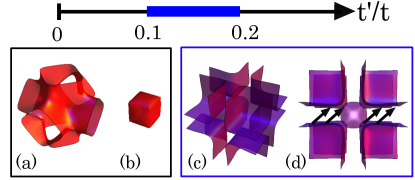
Figure 1: Fermi surfaces for the tight-binding model. In (a) and (b), we show the conduction and valence band Fermi surfaces, respectively, for $t^{\prime}/t=0$. For larger $t^{\prime}/t$, the conduction band Fermi surfaces become large and hole-like, as shown in (c) and (d) for $t^{\prime}/t=0.15$. The approximate nesting in the latter case is indicated schematically in (d).

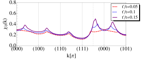
Figure 2: Zero frequency spin susceptibility for the tight-binding Hamiltonian for $t^{\prime}/t=0.05,0.1,0.15$, as a function of momentum ${\bf k}$ in the cubic Brillouin zone. Note that for the best nested situation, $t^{\prime}/t=0.15$, the susceptibility is sharply peaked close to the wavevector $2\pi(\frac{1}{4},\frac{1}{4},\frac{1}{4})$.

We now examine the Fermi surface in more detail in search of nesting tendencies. Fig.1 shows representative Fermi surfaces obtained from the tight-binding model as a function of the ratio $t^{\prime}/t$. With increasing $t^{\prime}/t$ from $0$ to $0.15$, the topology of the large Fermi surface is changing as seen in Fig.1(a), (c) and (d). In the absence of next-nearest-neighbor hopping $t^{\prime}/t=0$, the conduction band Fermi surface has an open topology as seen in Fig.1 (a). With increasing $t^{\prime}/t$, this Fermi surface becomes closed, comprising a large “pocket” centered at the zone corner. In the intermediate range (especially $0.1\leq t^{\prime}/t\leq 0.2$), the pocket resembles a cube, as seen in Fig.1(c) and (d) ((d) shows both valence band and conduction band Fermi surfaces). Contrary to the conduction band Fermi surface, the valence band Fermi surface retains its spherical topology for all $t^{\prime}/t$ ( see Fig.1(b)). The experimental Fermi surface of LaNiO₃ observed by Eguchi at al strongly resembles Fig.1(d).Eguchi et al. (2009)

The presence of large flat regions leads to nesting, and a tendency for CDW and/or SDW instabilities.Harrison (1980) A simple understanding of the effect of nesting is obtained from the Random Phase Approximation (RPA), in which the effect of interactions on the spin susceptibility is approximated by

$$\chi(\omega,{\bf k})=\frac{\chi_{0}(\omega,{\bf k})}{1-U\chi_{0}(\omega,{\bf k})},$$ (2)

where $\chi_{0}(\omega,{\bf k})$ is the non-interacting spin susceptibility, and we took for simplicity a spin and momentum-independent interaction $U$. An instability is signalled by a divergence of $\chi(0,{\bf k})$, which occurs on increasing $U$ when the denominator in Eq. (2) vanishes. This occurs for the ${\bf k}$ which maximizes $\chi_{0}({\bf k})\equiv\chi_{0}(0,{\bf k})$, which determines the wavevector of the spin ordering. In the case of perfect nesting, $E_{\bf q}=E_{\bf q+k}$ for every ${\bf q}$ on Fermi surface with the nesting vector ${\bf k}$, and the non-interacting susceptibility is itself divergent at this nesting wavevector, indicating an instability for arbitrarily small $U$. Although this is not true in general due to imperfect nesting, the flatness of the Fermi surface greatly strengths the tendency to instability.

To check this directly, we calculate the zero frequency spin susceptibility, which in general in the Matsubara formulation is given by

$$\chi_{0}(i\omega_{n},{\bf k}) = \langle S^{z}_{\bf k}S^{z}_{\bf-k}\rangle$$ (3)

$$= \frac{1}{2}\int\frac{d^{3}q}{(2\pi)^{3}}\frac{1}{\beta}\sum_{\Omega_{n}}\text{Tr}[G_{0}(i\Omega_{n},{\bf q})G_{0}(i(\Omega_{n}+\omega_{n}),{\bf q}+{\bf k})],$$ (4)

where the free electron Green’s function is defined as $G_{0}(i\omega_{n},q)=\langle c^{\dagger}_{\bf q}c_{\bf q}\rangle=(i\omega_{n}-E_{q})^{-1}$. More details are explained in Appendix.A. Fig.2 shows the calculated zero frequency spin susceptibility $\chi_{0}({\bf k})$ as a function of ${\bf k}$ for different ratios of $t^{\prime}/t$. As expected, the spin susceptibility is sharply peaked at a particular certain wave vector in the physical range of $t^{\prime}/t$. Specifically, $\chi_{0}({\bf k})$ for $t^{\prime}/t=0.15$ shows the highest peak at ${\bf k}={\bf Q}_{n}=2\pi(\frac{1}{4},\frac{1}{4},\frac{1}{4})$ which defines the nesting vector. Note that this is precisely the magnetic ordering wavevector (in the cubic convention) observed in the insulating low temperature phase of the nickelates. Estimating the instabilty from Eq. (2), we obtain $U_{c}\approx 1/\chi_{0}({\bf Q}_{n})\approx 2$ (see Fig.2).

III Hartree-Fock theory

III.1 Restricted Hartree-Fock Method

Having established the nesting wavevector, we proceed to a (restricted) Hartree-Fock treatment of the ordering and MIT. We include interactions in the two-band model via an on-site Coulomb term $U$ and Hund’s coupling $J_{H}$, defined from $H=H_{\rm tb}+H_{\rm int}$,

$$H_{\rm int} = U\sum_{i}n_{i}^{2}-J_{H}\sum_{i}{\bf S}_{i}^{2},$$ (5)

where $n_{i}=\sum_{a\alpha}n_{ia\alpha}$ and ${\bf S}_{i}=\sum_{a\alpha\beta}c_{ia\alpha}^{\dagger}\frac{{\bm{\sigma}}_{\alpha\beta}}{2}c_{ia\beta}$. As discussed earlier, what is important here, because of the nesting physics, is the interaction between states near the Fermi surface. As such, the $U$ and $J_{H}$ terms may be thought of as simply a convenient parametrization of the spin-independent and spin-dependent parts of these interactions, rather than literally in terms of atomic Coulomb and Hund’s rule terms.

To treat the problem in Hartree-Fock, we define a variational wavefunction as the ground state of a fiducial mean-field Hamiltonian, which has the form of a non-interacting two-band hopping model plus linear “potentials” arising from coupling to SDW and CDW order parameters. Experimental results predominantly favor collinear magnetic ordering, of the form

$$\langle{\bf S}_{i}\rangle\propto{\bf h}_{i}=\hat{z}{\rm Re}[{\bm{\psi}}e^{i{\bf Q}_{n}\cdot{\bf r}_{i}}]$$ (6)

with complex variable ${\psi}\equiv|\psi|e^{i\theta}$. Fig.3 shows different spin configurations which depend on the phase of $\theta$. For instance, $\theta=0$ corresponds to “site-centered” spin ordering in which the spin pattern is “up-zero-down-zero” moving along a cubic axis, while $\theta=\pi/4$ gives “bond-centered” ordering, and an “up-up-down-down” pattern. In the intermediate regime $0<\theta<\pi/4$, the order is “off-center” as shown in Fig.3(b).

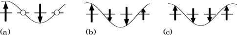
Figure 3: Spin configurations depending on the phase of $\psi$, $\theta$, along $\hat{x}$ axis. (a) shows “site-centered” spin ordering for $\theta=0$, (b) for intermediate $\theta=\pi/8$ and (c) is “bond-centered” ordering for $\theta=\pi/4$

As already discussed above and in Ref.Lee et al., 2011, a CDW order parameter will be induced with ${\bf Q}_{\rm cdw}=2{\bf Q}_{n}=\pi(1,1,1)$ as observed in experiment. This charge ordering is commonly known as “rock-salt” ordering and implies the electron density at site $i$ is represented as

$$\langle n_{i}\rangle\propto\rho_{i}=(-1)^{x_{i}+y_{i}+z_{i}}\Phi,$$ (7)

where $\Phi$ is an Ising-type order parameter for the charge ordering.

The full mean-field Hamiltonian from which the Hartree-Fock variational ground state is constructed then takes the form

$$H_{\rm var} = \tilde{H}_{\rm tb}+H_{\rm dw},$$ (8)

$$H_{\rm dw} = -\sum_{i}{\bf h}_{i}\cdot{\bf S}_{i}-\sum_{i}\rho_{i}n_{i}.$$ (9)

The local exchange field ${\bf h}_{i}$ and the charge ordering $\rho_{i}$ couple to the spin operator ${\bf S}_{i}$ and the electron number operator ${\bf n}_{i}$ respectively. Note that we allow additional freedom in the variational state by letting the hopping parameters renormalize. That is

$$\tilde{H}_{\rm tb}=H_{\rm tb}[t\rightarrow\tilde{t},t^{\prime}\rightarrow\tilde{t}^{\prime}].$$ (10)

The restricted Hartree Fock calculation proceeds by finding the ground state of $H_{\rm var}$:

$$H_{\rm var}|\Psi_{0}\rangle=E_{0}|\Psi_{0}\rangle,$$ (11)

with the constraint of quarter-filling, i.e. one electron per site, $\sum_{i}n_{i}=N$, where $N$ is the number of sites. The Hartree-Fock ground state $|\Psi_{0}\rangle$ is then a function of four dimensionless parameters: $\tilde{t}^{\prime}/\tilde{t},|\psi|/\tilde{t},\Phi/\tilde{t}$ and $\theta$. For each set of parameters, we calculate the variational energy

$$E_{\rm HF}=\langle\Psi_{0}|H|\Psi_{0}\rangle,$$ (12)

which is then minimized over the dimensionless parameters, for fixed physical parameters $t,t^{\prime},U$ and $J_{H}$.

To find $|\Psi_{0}\rangle$ in practice, we work in the reduce Brillouin zone (BZ) determined by the four site magnetic unit cell. We thereby end up with instead of two bands 8 magnetic ones, constructed from the different pieces of the original BZ folded into the magnetic one,

$$c_{na\alpha}({\bf k})=c_{a\alpha}({\bf k}+n{\bf Q}_{\rm sdw}),$$ (13)

with $n=0,1,2,3$ (for four magnetic sublattices), where $a$ is for two e_g orbitals and $\alpha$ is for spin $\uparrow\downarrow$. In this basis,

$${\tilde{H}}_{\rm tb}=\sum_{\bf k}^{{}^{\prime}}\sum_{n}{\tilde{H}}_{ab}({\bf k}+n{\bf Q}_{\rm sdw})c_{na\alpha}^{\dagger}({\bf k})c_{nb\alpha}({\bf k})$$ (14)

The prime on ${\bf k}$ sum means the sum over the reduced BZ. In the same way, the density wave Hamiltonian in ${\bf k}$ space is represented as,

$$H_{\rm dw} = \sum_{\bf k}^{{}^{\prime}}\sum_{n}\frac{\alpha\psi}{4}c_{n+1a\alpha}^{\dagger}({\bf k})c_{na\alpha}({\bf k})+{\rm h.c.}$$ (15)

$$\hskip 28.45274pt+\Phi c_{n+2a\alpha}^{\dagger}({\bf k})c_{na\alpha}({\bf k})$$

We then find the single-particle eigenstates by diagonalizing the $8\times 8$ matrix of the variational Hamiltonian Eq. (9), and construct $|\Psi_{0}\rangle$ by filling the states up to the Fermi energy, determined by the requirement of $1/4$ filling. It is then straightforward to express $E_{\rm HF}$ in terms of the single-particle states and occupation numbers, and perform the minimization procedure (see Appendix.B for more details).

III.2 Hartree-Fock Phase Diagram

III.2.1 Two SDW states

The resulting Hartree-Fock phase diagram for a typical situation with $t^{\prime}/t$=0.15 is shown in Fig. 4. We observe a metallic regime at small $U$ and $J_{H}$, and two main ordered phases with stronger interactions. For large $J_{H}$, site-centered SDW ordering with $\theta=0$ occurs, concurrent with strong charge order, generating an insulating state. This is natural because the large $J_{H}$ favors pairing of electrons into spin $S=1$ moments, requiring neighboring empty sites. More mathematically, such Hartree-Fock states minimize the Hund’s term. For large $U$, the bond-centered SDW with $\theta=\pi/4$ occurs instead. This is again natural because the $U$ term prefers uniform charge density, and with $\theta=\pi/4$ in the cubic system (which we discuss here) no CDW order occurs.

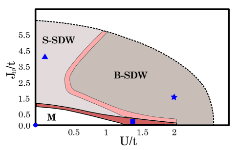
Figure 4: MIT bulk phase diagram for the model with cubic symmetry as a function of $U/t$ and $J_{H}/t$, with $t^{\prime}/t=0.15$. Here $U$ is the on-site Coulomb interaction, $J_{H}$ is the Hund’s coupling and $t$ is the nearest-neighbor hopping magnitude. The main phases which appear are a paramagnetic metallic state (M), metallic SDW (dark pink region close to M), insulating site-centered SDW (S-SDW), and semi-metallic bond-centered SDW (B-SDW). In between the S-SDW and B-SDW state, one observes an off-center SDW phase with $0<\theta<\pi/4$ (pink region). The blue colored shapes show the points for which the optical conductivity is plotted in Sec.VI

III.2.2 semi-metallic B-SDW

Somewhat surprisingly, the bond-centered SDW state remains semi-metallic even at relatively large $U$ within the Hartree-Fock approximation. Indeed, examination shows that the density of states is almost linearly vanishing approaching the Fermi energy in this region, with a small non-zero value at $E_{F}$, which decreases with increasing $U$. This unusual behavior arises from the specific “up-up-down-down” magnetic ordering in this phase. To understand it, recall that the cubic lattice, viewed from the $[111]$ direction, forms stacks of triangular lattice layers. In the limit of strong bond-centered ordering, the spins on each triangular plane are fully polarized. Moreover, electrons of one spin polarization are confined to a pair of parallel $[111]$ planes, which together forms a honeycomb lattice when connected by the dominant nearest-neighbor hopping $t$. Thus in the limit of large $U/t$ in the bond-centered SDW state, the appropriate tight-binding model is that of doubly degenerate e_g orbitals on honeycomb lattice.

$$H_{\hexagon}=-\sum_{ij}t^{ab}_{ij}c^{\dagger}_{ia}c_{jb}$$ (16)

This model has four orbitals per unit cell due to the doubly degenerate e_g orbitals and the bipartite honeycomb lattice. Fig.5(a),(b),(d) and (e) shows the dispersion and the DOS of this tight-binding model for the cases $t^{\prime}/t=0$ and $0.15$. Without second-nearest-neighbor hopping $t^{\prime}/t=0$, the result contains two bands which are identical to those of the canonical nearest-neighbor tight-binding model for graphene, possessing two Dirac cones with linear dispersion at Fermi level. The similarity with graphene has led to the suggestion that such systems might be used to engineer a topological insulator.Xiao et al. (2011) With increasing $t^{\prime}/t$, the DOS saturates at a small non-zero value approaching the Fermi level. This is because finite $t^{\prime}/t$ introduces both second-nearest-neighbor hopping and, more importantly, coupling between the honeycomb bilayers. The latter expands the Dirac points into small electron and hole pockets, in a similar manner as inter-layer coupling does in graphite.

III.2.3 effects of orthorhombicity

As discussed in Ref.Lee et al., 2011, the bond-centered ordering in the large $U$ region is actually unstable to orthorhombicity (GdFeO₃ distortion) , which is present in all the nickelates save LaNiO₃. This is expected on symmetry grounds to drive the SDW off-center. The off-centering in turn induces charge order. Thus at the symmetry level, when orthorhombicity is taken into account, the large $U$ region is completely consistent with experiment.

What of the metallicity in this region? In the graphene-like honeycomb bilayer, the Dirac point degeneracy is protected, as it is in graphene, by inversion symmetry. Inversion is indeed preserved by the bond-centered SDW in the ideal cubic system. It is, however, violated when both the SDW and orthorhombic distortion are present. Hence, we expect that orthorhombicity not only affects the centering of the SDW, it also tends to open a gap in the electronic density of states, converting the semi-metal to a true insulator.

We now study this microscopically. A leading effect of the orthorhombic distortion is expected to be a crystal field splitting of the e_g orbitals at each Ni site. Therefore, we add the on-site orbital splitting term

$$H_{\text{ortho}}=\sum_{i}{\bf D}_{i}\cdot c^{\dagger}_{ia}\tau_{ab}c_{ib}$$ (17)

Here we have suppressed the (diagonal) spin indices, and introduced Pauli matrices ${\tau}$ in the orbital space. Using the symmetries of the Pbnm space group of the orthorhombic structure, we find (see Appendix.C) that the “orbital fields” ${\bf D}_{i}$ are all expressible in terms of a single vector ${\bf D}$ :

$${\bf D}_{i}=((-1)^{x_{i}+y_{i}}D^{x},(-1)^{x_{i}+y_{i}}D^{y},D^{z})$$ (18)

For simplicity, we consider this term in the effective honeycomb lattice model, Eq.16, relevant for the large $U$ case. Fig.5 shows how the the DOS changes in the presence of an orthorhombic distortion. A gap indeed opens for sufficiently large ${\bf D}$, as plotted in Fig. 6.

III.2.4 Limitations of the restricted HF theory

Because we consider a restricted Hartree-Fock ansatz, some lower energy states that do not fit this ansatz may be missed in Fig.4. For example, near the onset of SDW order, at relatively weak interactions, there is the possibility of an incommensurate SDW. This may be expected since the best nesting vector determined by the maximum of the susceptibility is not exactly at the commensurate value, but rather at ${\bf Q}\approx 0.4\pi(111)$ (see Fig.2). Generally, commensurate states are preferred at strong coupling, and if incommensurate phases exist, they would be expected to change to the commensurate ones with increasing interaction strength, via a commensurate-incommensurate transition.Chaikin and Lubensky (2000)

We have also neglected the possibility of spontaneous orbital ordering, which could occur in the cubic model at large $U$. Indeed, orbital degeneracy is crucial to the semi-metallicity found in the B-CDW phase, as we have seen above via the introduction of orthorhombicity. Spontaneous orbital splittings (ordering) provide a mechanism for the cubic model to achieve a truly insulating state, which it must at sufficiently large $U$. However, we argue that the absence of any observed orbital ordering or Jahn-Teller distortion is evidence that this physics is not relevant for the nickelates.

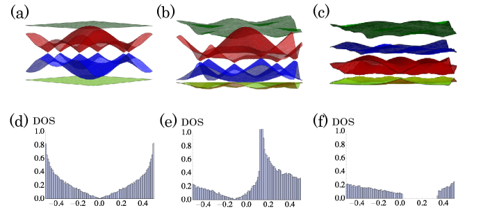
Figure 5: Dispersion (panels (a),(b) and (c)) and density of states (DOS, panels (d),(e),(f)) for the e_g tight-binding model on honeycomb lattice. In (a) and (d), $t=1$ and $t^{\prime}=0$, we observe Dirac points with clear linear dispersion and corresponding linear DOS. The Dirac cone is stable to small $t^{\prime}=0.15$ as shown in (b) and (e). In (c) and (f), an orbital splitting induced by the orthorhombic distortion of the lattice is included, with $t^{\prime}=0.15$ and ${\bf D}=1.5/\sqrt{3}(1,1,1)$. An induced gap is clearly seen.

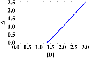
Figure 6: Plot of the single-particle gap $\Delta$ versus the orbital field $|D|$, for the honeycomb model with nearest-neighbor $t=1$ and $t^{\prime}=0.15$. Here we have arbitrarily taken the orbital field of the form ${\bf D}=(D,D,D)/\sqrt{3}$.

IV Strong coupling limit

The Hartree-Fock approach of the previous section is reasonable for weak to intermediate strength interactions, which we believe is most relevant for the more itinerant nickelates with R=Pr,Nd. For completeness, in this section we study the complementary limit of strong interactions, $U/t,J_{H}/t\gg 1$. Here the two-band model is suspect, so the connection to experiment is less clear. However, we can at least qualitatively attempt to address the question of the interplay of charge and spin order in the strong coupling regime. Specifically, note that in the more insulating nickelates, with R=Eu,Ho,Medarde et al. (1992) charge ordering appears first upon lowering temperature from the paramagnetic metallic state, with magnetism occuring only at lower temperature. Thus it seems that in these materials there is a separation of scales, with the primary mechanism for the MIT being charge ordering, and magnetism being secondary. In this section, we will see that this is indeed the case in one regime of the strong coupling limit of the two band model. The specific parameters of this region do not, however, seem very physical, supporting the idea that in the more insulating nickelates a description beyond the two band model is needed.

The strong coupling limit may be considered an expansion in the hopping $t,t^{\prime}$ about the limit $t=t^{\prime}=0$. In the extreme limit, the behavior is determined entirely by the “atomic” Hamiltonian $H_{\rm int}$ in Eq. (5), which can be solved independently at each site, subject to the constraint of proper total electron occupation (quarter filling). There are two regimes, determined by the parameter $\alpha=U/J_{H}$. For $\alpha>1/4$, the atomic ground state is one with one electron per site. In this regime every site is equivalent, and has four states available to it, due to the spin and orbital degeneracy. Further perturbation in $t,t^{\prime}$ will therefore result in a spin-orbital Hamiltonian of the Kugel-Khomskii type.

The other regime occurs when $\alpha<1/4$, and in this case the electrons prefer to segregate into two sets of sites with equal numbers in each: doubly occupied sites with total spin $S=1$, and empty sites. The ground state energy in this regime is $E_{0}=-(1-2\alpha)NJ_{H}$, where $N$ is the number of sites. Here there are two sorts of degeneracies. First, for $t=t^{\prime}=0$ the location of the paired sites is undetermined, so there is a degeneracy of $N!/[(N/2)!]^{2}$ associated with the different possible location of the pairs. In addition, for each of the paired sites, there are 3 spin states available.

In the remainder of this section, we will focus on this latter regime. Physically, we may consider the paired sites as bosons with spin $S=1$. By introducing hopping perturbatively, we may introduce hopping and interactions between the bosons. In the perturbative treatment, we will, in addition to $t/U,t/J_{H}\ll 1$, further assume $t^{\prime}/t\ll 1$, which simplifies the algebra considerably. Below, we argue that the leading effects of hopping, at $O(t^{2})$, induce charge ordering of the bosons, reducing the problem to an effective spin $S=1$ model. The spin degeneracy of the bosons is split only at the next non-trivial order, $O(t^{4})$. This qualitatively agrees with the separation of scales observed between charge and spin order in the nickelates.

IV.1 $O(t^{2}/J_{H})$: charge ordering

We first consider the effective Hamiltonian for the system at the leading non-vanishing order in perturbation theory, which is second order in hopping, for the case of $\alpha<1/4$. To formulate the perturbation theory , we treat the Hund’s and Coulomb part as the unperturbed Hamiltonian, $\mathcal{H}_{0}=H_{\rm int}$, and the hopping as the perturbation, $\mathcal{H}_{1}=H_{0}$. We denote the projection operator onto the ground state manifold of $\mathcal{H}_{0}$ at quarter filling by ${\mathcal{P}}$. If $|\Psi\rangle$ is an exact eigenfunction of the system with energy $E$, then its projection into the ground state subspace, $|\Psi_{0}\rangle=\mathcal{P}|\Psi\rangle$ satisfies

$$\left[E_{0}+\mathcal{P}\mathcal{H}_{1}\frac{1}{1-\mathcal{R}\mathcal{Q}\mathcal{H}_{1}}\mathcal{R}\mathcal{H}_{1}\right]|\Psi_{0}\rangle=E|\Psi_{0}\rangle,$$ (19)

where $\mathcal{R}=(\mathcal{H}_{0}-E)^{-1}$ is the resolvent and $\mathcal{Q}=1-\mathcal{P}$ . Eq. (19) is an implicit non-linear eigenvalue problem and we will only evaluate it perturbatively in $\mathcal{H}_{1}$, then it becomes

$$\mathcal{H}_{\rm eff}|\Psi_{0}\rangle \equiv (E-E_{0})|\Psi_{0}\rangle$$ (20)

$$\approx \mathcal{P}\mathcal{H}_{1}\sum_{n=0}^{3}(-1)^{n}\left(\mathcal{R}\mathcal{Q}\mathcal{H}_{1}\right)^{n}|\Psi_{0}\rangle,$$

where to this order of accuracy, we can safely approximate $\mathcal{R}\approx(\mathcal{H}_{0}-E_{0})^{-1}$.

The second order term in degenerate perturbation theory corresponds to $n=1$ in Eq. (20), in which electrons make two consecutive virtual hopping transitions. The terms for three different types of hops can be combined (see Appendix.D for more details), up to an additive constant, into

$$\mathcal{H}_{\rm eff}^{(1-3)} = \sum_{\langle ij\rangle}\big{[}\frac{4t^{2}}{J_{H}}\frac{1}{1-4\alpha}+$$ (21)

$$\frac{2t^{2}}{J_{H}}\frac{1}{5+4\alpha}\left(\vec{S}_{i}\cdot\vec{S}_{j}-1\right)\big{]}N_{i}N_{j}.$$

Eq. (21) gives the effective Hamiltonian at leading order for $\alpha<1/4$. To solve it, we note that $N_{i}$ commutes with $\mathcal{H}_{\rm eff}^{(1-3)}$ and is thus a good quantum number at every site. We then can easily see that the charge ordered states with $N_{i}=0,2$ on the two rock salt fcc sublattices saturate a lower bound on the energy, of $\mathcal{H}_{\rm eff}^{(1-3)}=0$. This follows because, since the eigenvalues of $\vec{S}_{i}\cdot\vec{S}_{j}$ are bounded by -2, hence the effective boson-boson repulsion (the term in the square brackets in Eq. (21)) obeys

$$V_{\rm eff}=\left\langle\frac{4t^{2}}{J_{H}}\frac{1}{1-4\alpha}+\frac{2t^{2}}{J_{H}}\frac{1}{5+4\alpha}\left(\vec{S}_{i}\cdot\vec{S}_{j}-1\right)\right\rangle>0.$$ (22)

Thus, regardless of the specific spin states of the boson pairs, their nearest-neighbor interaction is always repulsive for $0\leq\alpha<\frac{1}{4}$. The lower bound and hence charge order in the ground state follows.

IV.2 Magnetic interactions

Notably, although the effective interaction $V_{\rm eff}\sim t^{2}/J_{H}$ determines the charge order in the ground state (and defines the energy scale separating it from uniform states), the spin degrees of freedom on the doubly occupied sites remain undetermined at leading order. The spin physics is dictated by subdominant terms. Thus the appearance of charge order at a higher temperature than magnetism is a feature of this limit of the two-band model. Let us now consider the magnetic interactions in more detail.

First we focus on the spin exchange between nearest-neighbor sites on the fcc sublattice, i.e. second nearest-neighbor sites on the original cubic lattice. There are three lowest orders that we will consider: $O(t^{4}/J_{H}^{3})$, $O(t^{2}t^{\prime}/J_{H}^{2})$, $O(t^{\prime 2}/J_{H})$. Although the effects of the $t^{\prime}$ hopping is a relatively small correction to the dominant $t$ hopping, in the strong $J$ limit, it is not negligible because it can contribute at second and third order to the exchange between spins. Formally all these terms are on an equal footing if we take $t^{\prime}\sim t^{2}/J_{H}$. We combine the contributions from different orders together (see Appendix.D for more details). The total spin exchange between nearest-neighbor sites on the fcc sublattice is

$$J_{1}=-\frac{t^{4}}{J_{H}^{3}}\frac{1}{(1-4\alpha)^{2}}\big{[}\frac{8(5+4\alpha)}{(1-4\alpha)(5-4\alpha)}-\frac{5}{5+4\alpha}-\frac{1}{1-4\alpha}\big{]}+\frac{t^{2}t^{\prime}}{J_{H}^{2}}\frac{1}{1-4\alpha}\left[\frac{10}{5+4\alpha}+\frac{5}{1-4\alpha}\right]+\frac{t^{\prime 2}}{J_{H}}\frac{5}{5+4\alpha}.$$ (23)

Next we focus on the spin exchange between next nearest-neighbor sites. Calculation then shows

$$J_{2}=\frac{t^{4}}{J_{H}^{3}}\frac{1}{(1-4\alpha)^{2}}\left[\frac{16}{5-4\alpha}+\frac{8}{5+4\alpha}\right]$$ (24)

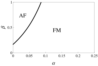
Figure 7: Phase diagram of the classical ground state as a function of two dimensionless parameters $\alpha\equiv U/J_{H}$ and $\beta\equiv t^{\prime}J_{H}/t^{2}$.

From the expression of $J_{1}$ and $J_{2}$, we obtain that if both $t^{\prime}$ and $\alpha$ are resonably small, there’s ferromagnetic interactions between nearest-neighbors and antiferromagnetic interactions between second nearest-neighbors on the fcc lattice. Case (1) for $O(t^{4}/J_{H}^{3})$ term is the dominant term for the ferromagnetic interaction. The negative sign for that case can be understood as arising due to the Hund’s rule coupling on the intermediate $k$ site, which prefers the two transferred virtual electrons to be in a triplet state. For the $J_{2}$ exchange, however, because $i,j,k$ are all along a single cubic axis, only one orbital can hop. For this reason, in the first hopping procedure (which is dominant) that contribute to $J_{2}$ it is impossible to obtain a triplet intermediate state, since two electrons in a single orbital must form an antisymmetric singlet. This explains the antiferromagnetic sign of this exchange.

Let us see what magnetic structure is expected from this exchange Hamiltonian. Since the fcc lattice is a Bravais lattice, we can use the Luttinger-Tisza method to find the classical ground states. We simply Fourier transform the exchange couplings to obtain the energy of spiral states with wavevector ${\bm{k}}$. One finds

$$E_{k} = -6J_{2}+4J_{2}\sum_{\mu=1}^{3}x_{\mu}^{2}+4J_{1}\sum_{\mu>\nu}x_{\mu}x_{\nu},$$ (25)

where $x_{\mu}=\cos k_{\mu}$. Since this energy is quadratic in the $x_{\mu}$, we can consider it as a quadratic form. The eigenvalues of the form are $8(J_{1}+J_{2})$ and $8J_{2}-4J_{1}$ (the latter is twofold degenerate). It is therefore positive definite if $J_{2}>{\rm Max}(-J_{1},J_{1}/2)$. When this is satisfied, the minimum energy states are those with $x_{\mu}=0$, i.e. $k_{\mu}=\pm\pi/2$. These are exactly the magnetic states observed experimentally. The phase diagram in Fig.7 shows the classical magnetic ground state for different values of $\alpha$ and $\beta\equiv t^{\prime}J_{H}/t^{2}$. We note that if $t^{\prime}=0$ ($\beta=0$) and $\alpha=0$, the ground state appears to be ferromagnetic. When $t^{\prime}$($\beta$) is included, the ferromagnetic $J_{1}$ interaction is decreased, and the antiferromagnetic state will be stabilized. For the region $\alpha<0.1$, the magnetic ground state is antiferromagnetic when $t^{\prime}\sim t^{2}/J_{H}$. It is remarkable that one can obtain in this way the same magnetically ordered state as found from the itinerant nesting picture.

IV.3 Comparison with weak coupling limit

According to the perturbation theory of the large Hund’s coupling, charge order first appears at $O(t^{2}/J_{H})$ and then magnetic ordering occurs due to perturbation at $O(t^{4}/J_{H}^{3})$,$O(t^{\prime 2}/J_{H})$ and $O(t^{2}t^{\prime}/J_{H}^{3})$ . Since the magentic ordering arises from a temperature scale smaller than the charge ordering phase, this agrees with the experimentally observed intermediate charge ordering phase without magnetism. On the other hand, in the weak coupling limit, the charge ordering is always slaved to the primary magnetic ordering.Lee et al. (2011)

V Confinement effects in thin films

The success of the Hartree-Fock theory in reasonably predicting the charge and spin ordering in the more itinerant nickelates undergoing a MIT suggests that the approach may also be profitably applied to films. Recently, various growth issues have been overcome leading to epitaxial films of good quality on several substrates with layer by layer control. One may expect that the MIT and related charge and spin ordering can be strongly modified in thin films, due to both distortions (dependent on details of the substrate and growth conditions), effects of changes in chemistry at interfaces, and to quantum confinement effects. Because of the difficulty of controlling the former two effects (which in any case are better studied by first principles methods), we focus here entirely on the latter, and consider in this section the simplest possible model of a finite thickness film. That is, we simply take the bulk tight-binding Hamiltonian and apply it to a finite thickness slab consisting of $L$ unit cells in the confined direction, with effectively “vacuum” outside the slab, i.e. open boundary conditions. Given the importance of Fermi surface shape in determining the nesting properties, we expect that quantum confinement alone can significantly modify the MIT properties and the ordering in the insulating state.

V.1 Single Layer, $L=1$

First of all, we consider the extreme case of a single NiO₂ layer, following the methods used for the bulk. Here and throughout this section, we will neglect the symmetry-lowering effects that must be present in such a two dimensional structure, and in particular any tetragonal orbital splitting which is likely to be the dominant effect of this type. With this proviso, the Fermi surface and nesting properties are shown in Fig.9(a). The two dimensional Fermi surfaces show large flat regions similar to the bulk case. The zero frequency spin susceptibility, $\chi_{0}^{\rm 2d}(k)$, is shown in Fig.9(e) (see Appendix.A). It is sharply peaked at ${\bf Q}_{\rm sdw}^{\rm 2d}=2\pi(\frac{1}{4},\frac{1}{4})$. Repeating the Hartree-Fock calculations for this case, using this SDW vector, we obtain the phase diagram in Fig.8(a). The results are quite similar to the bulk case, except that the bond-centered SDW is insulating in this case, as the honeycomb lattice structure does not arise for a single square lattice layer. Somewhat surprisingly, the location of the MIT $(U/t)_{c}\approx 2$ at $J_{H}/t=0$ remains almost unchanged from the bulk case. Naïvely, one would expect a decrease in $(U/t)_{c}$ in 2d, because the bandwidth is reduce by confinement. We attribute the lack of such a decrease to decreased nesting in the two dimensional case, as can be seen by comparing Fig.2 and Fig.9: the susceptibility has a higher peak in bulk than in the single layer.

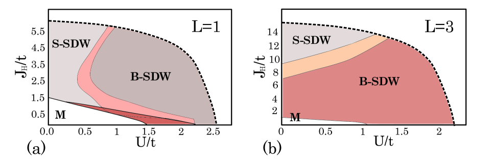
Figure 8: Panel (a) shows the zero temperature phase diagram for a single layer $L=1$ with the nesting vector ${\bf Q}^{\rm 2d}_{\text{sdw}}=2\pi(\frac{1}{4},\frac{1}{4})$. As in the bulk case, the paramagnetic metallic phase (M) is stable for weak interactions. The dark pink region indicates a metallic SDW state, and the light pink region indicates an insulating off-center SDW. Panel (b) shows the phase diagram for three layers, $L=3$, with the nesting vector ${\bf Q}^{L=3}_{\text{sdw}}=2\pi(\frac{1}{4},0,0)$. This nesting vector leads to a metallic B-SDW phase, which persists even for large $U/t$. The yellow region between the S-SDW and B-SDW phases is a metallic off-center SDW.

V.2 Intermediate thickness films

We now consider the intermediate cases with $L\geq 2$ NiO₂ layers along the $\hat{z}$ direction. In this case, the single-particle states can be taken as standing waves in the vertical ($\hat{z}$) direction, with $k_{z}=\pi l/(L+1)$ where $l=1,2,\cdots,L$. One obtains correspondingly $2L$ subbands ($2$ arising from the orbital degeneracy), each of which may have a Fermi surface. The calculated non-interacting Fermi surface and spin susceptibility for several values of $L$ are shown in Fig.9 (see Appendix.A for more details of the calculation of the spin susceptibility).

From Fig.9(g), we see that the peak of the susceptibility varies considerably and in a non-monotonic fashion with $L$. While the case $L=2$ (orange points in Fig.9(f)) is quite similar to the result for the single layer, $L=3,4$ are considerably distinct. For larger $L$, there is a slower variation of behavior, and by increasing the thickness to $L=30$ (purple points in Fig.9(f)), the bulk behavior (black line in Fig.9(f)) is almost perfectly recovered. Thus we expect particularly distinct phase diagrams for the cases $L=3,4$, and focus on these below.

V.2.1 $L=3$

For $L=3$, one observes comparable peaks in the susceptibility at two wavevectors: ${\bf Q}=\pi/2(100)$ and ${\bf Q}=\pi/2(110)$. The former is quite distinct from the ordering in the single layer and bulk cases. To decide amongst the two possibilities, we compared the variational energy in the Hartree-Fock approximation for the two choices, and found that, over the full range of $U$ and $J$, the total energy is lower for ${\bf Q}=\pi/2(100)$. Thus the model predicts quite distinct ordering in the trilayer case.

The full Hartree-Fock phase diagram, assuming this wavevector, is shown in Fig.8(b). Details of the calculations for finite $L$, which are somewhat complicated by the many subbands, are given in App.B. Once again both site-centered and bond-centered SDW states appear, but the site-centered SDW occurs here only at very large values of the Hund’s coupling, $J_{H}/t\gtrsim 10$, making it probably entirely unphysical. Another distinction from the cases discussed previous is that the bond-centered SDW for $L=3$ appears to be fully metallic. This is because the SDW with wavevector ${\bf Q}=\pi/2(100)$ describes stripes of electrons with all spins parallel in vertical stripes along the $y$ direction. Thus the electrons are free to hop in this direction – actually they form “ladders” of two parallel spin-aligned chains – and one has a sort of quasi-one-dimensional metallic state. Instabilities of the one-dimensional ladders would probably be expected beyond the Hartree-Fock approximation, and could lead to further charge/spin/orbital ordering and insulating behavior, but this is not within the scope of our study.

V.2.2 $L=4$

One more noticeable feature in the spin susceptibility plotted Fig.9(f), is the large ${\bf Q}\approx 0$ peak for $L=4$ (see blue points). The ${\bf Q}=0$ (uniform) susceptibility is simply proportional to the density of states, which is apparently enhanced for this film thickness. The origin of this enhancement is seen by inspecting separately the Fermi surfaces associated with individual sub-bands with discretized $k_{z}=\pi l_{z}/(L+1)$, shown in Fig.10. One sees that the $L=4$ case is unique in having three distinct Fermi surfaces (two hole and one electron) for the $l_{z}=1$ sub-band. Since the density of states is proportional to the Fermi surface area, this explains the observed enhancement. Some understanding of this is obtained by inspecting the bulk Fermi surface, Fig.1(d). It contains a large hole-like surface which has rather flat faces, parallel to [001] planes. For the specific case $L=4$ and $l_{z}=1$, the discretized $k_{z}=0.2\pi$ cuts across this rather flat when $l_{z}=1$. As a result, the flat face, leading to the multiple two-dimensional sub-band Fermi surfaces. This enhanced density of states could potentially lead to ferromagnetism for this case, but since ferromagnetism is notoriously over-estimated by the Hartree-Fock approximation, we do not pursue this further here.

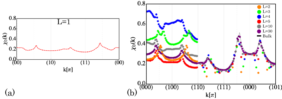
Figure 9: The zero frequency spin susceptibility, $\chi_{0}({\bf k})$, for finite thickness slabs of $L$ layers, for the free electron tight-binding Hamiltonian with $t^{\prime}/t=0.15$. Plot (a) shows the purely two-dimensional single layer case. Here $\chi_{0}({\bf k})$ is sharply peaked at ${\bf k}={\bf Q}_{\text{sdw}}^{2d}=\pi/2(11)$. Plot (b) shows several cases with varying thickness with $2\leq L\leq 30$, compared with the bulk case $L=\infty$. One sees that large $L=30$ (purple dots) agrees well with the bulk susceptibility (black solid line). For smaller $L$, we see that the nesting properties change considerably. This is especially pronounced for $L=3$ (green points), for which $\chi_{0}({\bf k})$ is sharply peaked at ${\bf k}={\bf Q}\approx\pi/2(100)$, and for $L=4$ (blue points), for which it is peaked at ${\bf k}\approx 0$.

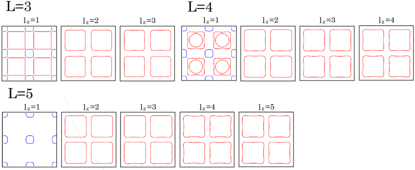
Figure 10: The Fermi surfaces for different subbands in the $k_{x}$-$k_{y}$ plane with discretized $k_{z}=\pi l_{z}/(L+1)$ for the cases $L=3,4$ and $5$. The blue (red) lines correspond to conduction (valence) subbands. In the case $L=4$, we see two valence subband Fermi surfaces at $k_{z}=0.2\pi$ ($l_{z}=1$), which is responsible for an enhancement of the DOS at Fermi energy.

VI Discussion

In the prior sections, we have studied a minimal two band model for the perovskite nickelates, with a focus on the MIT and the spin and charge ordering in the insulating state.

VI.1 Do we need the oxygen orbitals?

In the minimal model used in this paper, we have eliminated the oxygen orbitals to obtain an effective two orbital Hubbard model. Several papers in the literature, however, claim that the oxygen states are crucial for the physics of the nickelates. Here we will discuss this issue, and argue that the importance of explicit inclusion of the oxygen states depends upon the questions being asked.

In general, in the Fermi liquid paradigm, which applies to weakly to moderately correlated itinerant systems, the behavior of the electrons is dictated by the vicinity of the Fermi surface(s) only, and by the effective interactions amongst these states near the Fermi surface. The great insight of Landau in developing Fermi liquid theory was that the actual wavefunctions of these “quasiparticle” states are largely unimportant. Thus when it applies, any model which properly mimics the band dispersion near the Fermi surface (and its symmetry), and which captures sufficiently the interactions amongst the near-Fermi surface states, serves to correctly model the electronic behavior. It is well established now that LaNiO₃, the metallic end-member of the RNiO₃ series, has a Fermi surface which is obtained from the intersection of just two bands with the Fermi energy. These bands have $e_{g}$ character, which can be mimicked by the minimal tight-binding model used in this paper. Provided a band picture of the important electronic states near $E_{F}$ is adequate, this basis is sufficient to describe the nickelates. The extent of the microscopic oxygen versus nickel character of the states is subsumed into the Bloch wavefunctions, which do not appear in the band Hamiltonian, and to a lesser extent in the effective interactions. We conclude that for low to intermediate energy properties for which the two-band description is adequate, explicit treatment of the oxygen states is not important.

However, one may ask questions – and conduct experiments – for which the oxygen states are obviously essential. For instance, inelastic x-ray scattering can measure the relative fraction of Ni²⁺ and Ni³⁺ occupation of the Ni 3d states. Estimates for NdNiO₃ is that there is as much as 40% Ni²⁺. By neutrality, the Ni²⁺ can only arise through the presence of holes on the oxygen states. This implies the Bloch wavefunction associated with the the “oxygen bands” and “nickel bands” have in fact considerably mixed character. However, this does not affect the reliability of the two band model for the states near the Fermi energy. Indeed, the measurement of the Ni valence state is actually a measure of the occupied states, and hence is really related to the character of the filled valence band Bloch wavefunctions, not that of the near-Fermi surface states. Of course, by orthogonality, if the nominally oxygen states have mixed character, so too must the nickel states.

Other high energy questions may be sensitive to the oxygen character. For instance, let us consider the properties of an interface. In standard semiconductor systems, an interface can be understood through band diagrams, which include only the energies of the bands, and not their wavefunctions. Thus when this approach applies, the oxygen character is not important. In fact, band diagrams rely upon a semiclassical treatment which assumes that the electrostatic potential, carrier density, etc. vary slowly with respect to the lattice spacing. This in turn is correct in semiconductors due to their small effective mass and large dielectric constant. There is no need for this to apply to nickelate interfaces.

In fact, it would be natural to expect a change in the oxygen character at an interface.Han et al. (2010) Consider an interface with a band insulator such as LaAlO₃ (LAO), in which there are no 3d orbitals near the Fermi energy. By neutrality, in LAO the oxygen valence should be “exactly” (or at least much more so than in the nickelates) O^2-. This implies that the Ni 3d orbitals in the plane adjacent to the LAO are less able to hybridize with the intervening oxygens, since these states are “blocked”. One can consider a simple model in which this physics is accounted for by ascribing an oxygen orbital energy $\epsilon_{p^{\prime}}$ for the intervening oxygens which is lower (so that here the electrons are more strongly bound to their oxygen) than the energy $\epsilon_{p}$ for the same orbitals inside the nickelate, i.e. $\epsilon_{p^{\prime}}<\epsilon_{p}$. The larger energy separation $\epsilon_{d}-\epsilon_{p^{\prime}}>\epsilon_{d}-\epsilon_{p}$ for the interfacial states implies reduces mixing of the nickel and oxygen states. Thus we expect that the Ni²⁺ character of the interfacial nickel ions should be reduced. As already remarked, this is a high energy property, related to the occupied states. However, the reduced mixing has implications at low energy as well. It implies reduced level repulsion between the 3d (specifically the d${}_{z^{2}}$) and 2p states, so that the partially filled orbitals corresponding to the near Fermi energy states should be lowered relative to bulk nickelates near the interface. That is, the conduction electrons feel an attraction to the d${}_{z^{2}}$orbitals in the interfacial NiO₂ plane. Note that, although oxygen physics induces corrections to its Hamiltonian parameters, the two-orbital model remains valid even for the interface.

This physics may be relevant to recent experiments on LNO heterostructures. Several experiments have indicated the formation of an insulating state for very thin LNO films with only a few unit thickness. This appears at odds with the calculations in Sec. V, which find that the metal-insulator transition point is largely unchanged by confinement, even for very thin films. This model, however, neglects the induced orbital potential at the interface. One would expect this orbital potential to partially polarize the orbitals at the interface in favor of the d${}_{z^{2}}$ states which conduct poorly in the xy plane. Moreover, the shift of these orbitals renders inter-layer tunneling non-resonant, which will further reduce the kinetic energy. Thus it is natural to expect the insulating state to be enhanced by this effect. In the future, we plan to investigate this in more detail by including the interfacial orbital attraction explicitly in the Hartree-Fock calculation.

VI.2 Strong versus intermediate correlation

In this paper, we have contrasted the limits of weak to intermediate correlation (and Hartree-Fock theory) and strong correlation (the perturbative approach in Sec. IV). It was argued that the strong coupling limit seems not very realistic. However, there are indications that something beyond the weak coupling view is needed, at least for the more insulating nickelates, with R=Lu,Ho,Y. In these materials, the charge ordering and insulating transition occurs above 500K but magnetism only sets in around 100K. A factor of 5 or more discrepancy between these two scales is hard to reconcile with a weak-coupling picture. One type of strong-coupling picture is discussed by Anisimov et alAnisimov et al. (1999), in which the nickel charge state is regarded as Ni²⁺, which forms an $S=1$ spin, while the mobile charge is actually in the form of holes on the O sites. The corresponding model would be a type of underscreened Kondo lattice. Charge ordering of the type seen in experiment is certainly possible, and would be viewed as the formation of collective Kondo singlets between two holes and a Ni²⁺ spin on half the lattice sites.Sawatzky et al. To our knowledge, whether this actually occurs for a Kondo model of this type has not been established theoretically. This is an interesting problem for future study. A likely issue with such a Kondo description is that the band structure appears very different from the bands with $e_{g}$ character predicted and observed in LaNiO₃. Instead, the itinerant carriers must arise from oxygen bands, and it is not clear why this should in any way mimic the $e_{g}$ structure. But perhaps the bands in LuNiO₃ etc. are radically different from those in LaNiO₃. If so, this should be testable experimentally.

Some sort of intermediate coupling picture is also possible. Indeed, even if the most insulating materials are at strong coupling, and, as we have suggested, PrNiO₃ and NdNiO₃ are better thought of in the SDW (weak to intermediate coupling) limit, then there are compounds in between. Here presumably a full description with all the orbital involved and charge fluctuations allowed in all orbitals is needed, and there is little simplicity to be found. Probably an approach which combines elements of ab initio theory and reasonable but ad-hoc treatment of interaction physics such as DMFT is the best in this regime.Han et al. (2011) In this situation, it will unfortunately probably be difficult to identify any single mechanism for charge ordering.

In our opinion, it is likely that one physical effect we have not so far discussed, the coupling to lattice phonons, is important. The Kondo singlet formation mentioned above would obviously benefit from a contraction of the neighboring oxygens around the Ni²⁺ spin in question. Indeed, it is this contraction which is actually observed experimentally, rather than any real electric charge density. The same local phonon mode which would couple to the Kondo singlet would also favor charge ordering in the intermediate coupling view. It may be that this electron-phonon interaction gives a reasonable mechanism for the more insulating nickelates.

VI.3 Experimental signatures

It is desirable to understand how the different scenarios might be distinguished experimentally. We will focus here primarily on the expected consequences in the itinerant regime, as the primary focus of this work. However, we briefly discuss expectations for the strong coupling limits. In the strong coupling pictures, we would presumably expect the insulating states to have a full gap to electron and hole quasiparticles. Moreover, local $S=1$ moments would be well-formed on half the Ni sites (forming an fcc sublattice), prior to ordering into an antiferromagnetic ground state. With these site-center local spins, it seems difficult to imagine an antiferromagnetic state with the symmetry of the bond-centered or off-center SDW, and we would expect a site-centered SDW (antiferromagnetic) order. This particular symmetry could be distinguished by a careful determination of local moments at all the nickel sites from neutron or NMR/$\mu$SR measurements.

Turning now to the itinerant regime, we consider the experimental consequences of the nesting scenario. First we discuss the thermal phase transition. In this limit, since the SDW drives the charge order, the two types of order should set in simultaneously at a single critical temperature. In Ref.Lee et al., 2011, it was shown that this transition is theoretically expected to be first order for several reasons. These two observations are consistent with experiment.

More detailed comparison can be made with electronic structure. We discuss in particular the implications of the nesting scenario for dc transport and optical measurements in the following.

VI.3.1 Transport anisotropy

Transport is an important probe of the electronic structure. In the nesting picture, the SDW order is directly and strongly coupled to the quasiparticles, and hence should strongly influence the transport. The most qualitative feature of this coupling is that the SDW order imposes its lower lattice symmetry, and in particular, spatial anisotropy, upon the quasiparticles. In contrast, within the strong coupling view, the charge ordering is dominant, and this charge ordering itself is not anisotropic (it doubles the unit cell but is compatible with cubic symmetry). We therefore expect that, when the nesting picture is valid, prominent transport anisotropy should be observed to set in for $T<T_{\rm MIT}$.

We focus first on the bulk case, for which the SDW wavevector ${\bf Q}_{\rm sdw}=2\pi(1/4,1/4,1/4)$ obviously breaks cubic symmetry. As discussed in Sec. III.2.2, the electronic structure in the B-SDW phase is describable as a set of weakly coupled honeycomb [111] bilayers, leading (neglecting orthorhombicity) to a semi-metallic state. Hence we expect the B-SDW ordering to be accompanied by strong electrical anisotropy, with much larger conductivity within the [111] plane than normal to it.

We have calculated this conductivity at zero temperature using the Hartree-Fock quasiparticle Hamiltonian. From the Boltzmann equation within relaxation time approximation, one has

$$\sigma_{\mu\nu}=\sum_{n}e^{2}\tau\int\frac{d^{3}k}{8\pi^{3}}[-f^{\prime}(\epsilon_{n})]v_{n,\mu}(k)v_{n,\nu}(k),$$ (26)

where $\tau$ is a constant relaxation time, $f$ is the Fermi distribution $f(\epsilon)=1/(e^{\beta(\epsilon-\mu)}+1)$ and $v_{n,\mu}=\partial\epsilon_{n}(k)/\partial k_{\mu}$, where $n$ is a band index. We have a total of 8 bands (2 e_g orbitals $\times$ 4 magnetic sublattices = 8), and the band energies and velocities must be found numerically. Using $k\cdot p$ perturbation theory,Kittel and McEuen (1986) one has:

$$v_{n,\mu}(k)=\langle\psi_{nk}|\frac{\partial{\sf H}(k)}{\partial k_{\mu}}|\psi_{nk}\rangle,$$ (27)

where ${\sf H}(k)$ is the 8$\times$8 matrix Bloch Hamiltonian. From the above formulae, we calculated the conductivity $\sigma_{\parallel}$ parallel to the [111] axis and $\sigma_{\perp}$ normal to it. The ratio is plotted in Fig. 11 for the B-SDW state. As expected, a large anisotropy is observed once a significant magnetic order develops.

Figure 11: Bulk conductivity anisotropy in the B-SDW state, as a function of the amplitude $|\psi|$ of the SDW order parameter.

Note that the same result would be expected to obtain for a thick film, where the behavior is predominantly bulk-like. In this case, the measureable quantity is the effective two-dimensional conductivity tensor for the plane of the layer, which is usually an [001] plane. By symmetry, we expect the principle axes of the 2d conductivity to be the [11] and [1-1] directions, with different conductivities along each in the SDW state. Note that in practice this is complicated by the effects of orthorhombicity, which already should induce transport anisotropy even in the metallic state. However, we expect that this intrinsic anisotropy is probably mild, and that a pronounced effect due to SDW ordering should be observable below $T_{\rm MIT}$.

For thin films, confinement effects may contribute to or modify the anisotropy. For instance, in the three layer case, we observed a change in the nesting wavevector to ${\bf Q}_{L=3}=2\pi(1/2,0,0)$. In this state, the anisotropy axes imposed by the SDW are different. In particular, an“up-up-down-down” magnetic configuration along the $\hat{x}$ axis is stabilized, so that the spin polarized electrons are free to hop along ${\hat{y}}$ direction. Hence, in this case the low and high conductivity axes are the $[10]$ and $[01]$ axes, respectively. This is shown in Fig.12, in which the magnitude of SDW, $|\psi|$, is varied while fixing $\tilde{t}=1,\tilde{t}^{\prime}=0.15,\theta=\pi/4$ and $\Phi=0$. Indeed, in this case the anistropic behavior is even more pronounced, for in the model the “hard” axis conductivity $\sigma_{xx}$ actually vanishes at $T=0$ in the limit of large SDW gap, while $\sigma_{yy}$ saturates to a constant for arbitrarily large $|\psi|$, because the spin polarized electrons are free to hop along $\hat{y}$ direction. In this case, the formation of the SDW opens the Fermi surface.

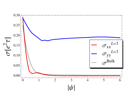
Figure 12: Electrical conductivity for $L=3$ and bulk with fixed $\tilde{t}=1,\tilde{t}^{\prime}=0.15,\theta=\pi/4$ and $\Phi=0$. The isotropic conductivity in the bulk case (black line), $\sigma^{\text{Bulk}}$, decreases to zero with as a gap in the DOS develops with increasing SDW order. For the three layer case, $L=3$, the conductivity shows a large anisotropy in the $x-y$ plane once the SDW develops.

VI.3.2 Optical conductivity

Optical conductivity is an other important probe of electronic structure. For LaNiO₃, which is metallic at all temperature, experiment shows a reduced Drude peak compared to band theory,Ouellette et al. (2010) which may be considered as evidence of moderately strong correlation. However, apart from this quantitative renormalization of the low energy Drude part, the theoretical optical conductivity obtained from the simple two e_g band model reproduces experiment fairly well up to $\omega\approx 2eV$.Ouellette et al. (2010) Applying the same analysis to the magnetically ordered phases in our bulk phase diagram, Fig.4, we obtained strikingly different results as a consequence of SDW formation.

The calculations are made using standard linear response theory within the Hartree-Fock variational Hamiltonian. From the Kubo formula, the real part of optical conductivity $\sigma_{\alpha\beta}(\Omega,{\bf k})$ is related to the imaginary part of current-current correlation $\Pi_{\alpha\beta}(\Omega,{\bf k})$: Mahan (2000)

$$\sigma_{\alpha\beta}=\frac{i}{\omega}\int\frac{d^{3}k}{(2\pi)^{3}}\Pi_{\alpha\beta}(\Omega,{\bf k})+\frac{n_{0}e^{2}}{m}\delta{\alpha\beta}$$ (28)

with wave vector ${\bf k}$, frequency $\Omega$, average density $n_{0}$ and electron mass $m$. The current-current correlation function with imaginary frequency $i\Omega_{l}$ is defined as

$$\Pi_{\alpha\beta}(i\Omega_{l},{\bf k})=\frac{2}{vol}\sum_{abcd}j_{\alpha}^{ab}({\bf k})j_{\beta}^{cd}({\bf k})\frac{1}{\beta}\sum_{n}G_{ad}(i\omega_{n}+i\Omega_{l},{\bf k})G_{cb}(i\omega_{n},{\bf k}).$$ (29)

At zero temperature, this can be calculated from the spectral representation (see Appendix.E),

$${\rm Im}[\Pi_{\alpha\beta}(\Omega,{\bf k})]=\sum_{mm^{\prime}}\phi_{m}^{a*}\phi_{m^{\prime}}^{b}\phi_{m^{\prime}}^{c*}\phi_{m}^{d}\int\frac{d\omega}{\pi}A_{m}(\omega)A_{m^{\prime}}(\omega+\Omega)(n_{F}(\omega)-n_{F}(\omega+\Omega)),$$ (30)

where $A_{m}(\omega)=\gamma/[(\omega-E_{m}+\mu N)^{2}+\gamma^{2}]$, with $\gamma$ a small scattering rate (imaginary part of the first order self-energy correction ${\rm Im}[\Sigma(\omega_{n})]=-i\gamma sgn(\omega_{n})$) added by hand, and $\phi_{m}^{a}({\bf k})$ is the $a$ component of $m$th eigenstate. $n_{F}(\omega)=1/(e^{\beta\omega}+1)$ is Fermi distribution.

Fig.13 shows the optical conductivity calculated in this way for each of the different phases (taken at the spots marked by symbols in the phase diagram in Fig.4). The above-mentioned comparison of theory and experiment for the paramagnetic metallic state is shown in panel (a), taken from Ref.Ouellette et al., 2010. The development of SDW order strongly suppresses the Drude peak, as expected, which can already be seen in the metallic SDW state when the density of states at the Fermi energy is still non-zero (but small), Fig.13 (b). Interestingly, a small peak appears instead at $\omega/t\sim 0.3$. This peak arises from a transfer of spectral weight from low frequency to above the SDW gap. Panel (c) shows $\sigma(\omega)$ for the B-SDW state, which has a semi-metallic band structure. One observes a linear increase of ${\rm Re}[\sigma(\omega)]$ for small frequency $\omega$, which is similar to the behavior expected from the Dirac points in graphene, and indeed arises from the honeycomb [111] bilayer structure of the spin-polarized regions, as discussed in Sec. III.2.2. Here we have plotted the powder-average conductivity, since the full tensor is anisotropic as discussed above. This calculations has neglected orthorhombicity, which would introduce a gap at low energy and thereby interupt at least part of the linear region. However, a linear increase of $\sigma(\omega)$ at low frequency was indeed seed in bulk experiments on NdNiO₃ below the transition temperature.Katsufuji et al. (1995) Finally in Fig.13(d), we plot the optical conductivity for for large Hund’s coupling $J$, in the S-SDW where strong charge order is present. A large gap opens in the spectrum, resulting in zero ${\rm Re}[\sigma(\omega)]$ up to $\omega/t\approx 1$.

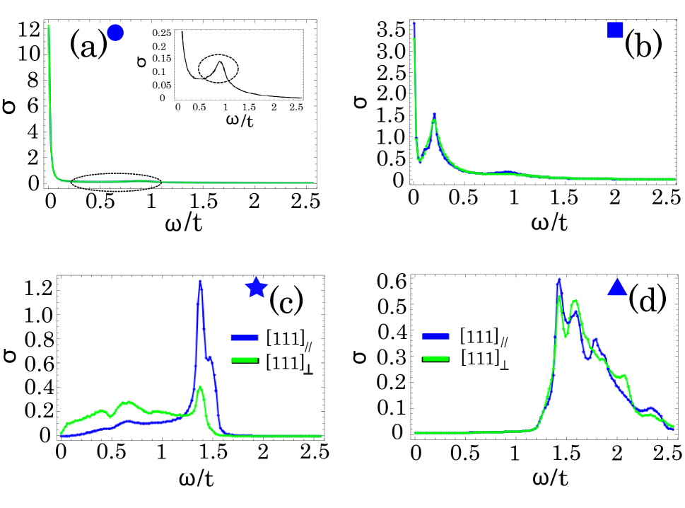
Figure 13: The real part of the optical conductivity, $\sigma(\omega)$, for each phase (colored star) in the bulk phase diagram (see Fig.4). In (a), the paramagnetic metallic phase shows a large Drude peak and a small hump (see inset plot). The hump is related to a region of large DOS for interband transitions (see Ref.Ouellette et al., 2010). In (b), the metallic SDW phase has a reduced but non-zero Drude peak and a small second peak due to the SDW gap. Plot (c) shows the case of the semi-metallic B-SDW phase, for which a linear increase of $\sigma(\omega)$ for small frequency $\omega$ is found, related to the linear dispersion near the Fermi level. It also shows strong anisotropy between the conductivity $\sigma_{[111]_{\parallel}}$ (along the [111] direction) (blue line) and $\sigma_{[111]_{\perp}}$ (perpendicular to [111]) (green line). In plot (d), a large gap is visible in the S-SDW phase.

VI.4 Summary

We have presented a theoretical analysis of the metal-insulator transition in the nickelates from a minimal two-band model and Hartree-Fock theory, which we argued is appropriate for the itinerant limit of weak to intermediate correlation. This picture of the metal-insulator transition can be tested in various ways, as suggested above, and appears to us to be the most consistent one for the materials NdNiO₃ and PrNiO₃, located close to the zero temperature MIT phase boundary. For the more insulating nickelates, a different type of theory is required, involving stronger correlation and possibly an important role for electron-lattice coupling. Both further theoretical work in clarifying the mechanism for the MIT transition in those materials, and experimental work which can test the itinerant picture (such as measurement of transport anisotropy), would be very desireable. Finally, we have shown that quantum confinement alone cannot explain a Mott insulating in ultrathin LaNiO₃ films, and suggested a physical mechanism by which the observed insulating state might obtain. It will be interesting to pursue this question further in the future.

Appendix A Dynamical Spin Susceptibility for Free Electrons ${\bm{\chi}_{0}(\Omega,k)}$

In this section, we derive the dynamical spin susceptibility for free electrons both for bulk and finite layers. In general, dynamical spin susceptibility for Matsubara frequency $i\Omega_{n}$, and wave vector $k$ can be represented as following

$$\chi_{0}(i\Omega_{n},{k}) = \langle S^{z}_{\bf k}S^{z}_{\bf-k}\rangle$$ (31)

$$= \frac{1}{N}\langle\sum_{{\bf rr^{\prime}}}S^{z}_{\bf r}S^{z}_{\bf r^{\prime}}e^{i{\bf k(r-r^{\prime})}}\rangle$$ (32)

$$= \frac{1}{N}\langle\sum_{\bf rr^{\prime}}\sum_{\alpha\beta,\alpha^{\prime}\beta^{\prime}}\frac{1}{4}c^{\dagger}_{\bf r\alpha}c_{\bf r\beta}c^{\dagger}_{\bf r^{\prime}\alpha^{\prime}}c_{\bf r^{\prime}\beta^{\prime}}\sigma^{z}_{\alpha\beta}\sigma^{z}_{\alpha^{\prime}\beta^{\prime}}e^{i{\bf k(r-r^{\prime})}}\rangle$$ (33)

$$= \frac{1}{N}\langle\sum_{\{\bf q_{i}\}}\sum_{\bf rr^{\prime}}\sum_{\alpha\alpha^{\prime}}\frac{1}{4N^{2}}c^{\dagger}_{\bf q_{1}\alpha}c_{\bf q_{2}\alpha}c^{\dagger}_{\bf q_{3}\alpha^{\prime}}c_{\bf q_{4}\alpha^{\prime}}(-1)^{\alpha+\alpha^{\prime}}e^{i(\bf q_{1}-q_{2}+k)r}e^{i(\bf q_{3}-q_{4}-k)r^{\prime}}\rangle$$ (34)

$$= \frac{1}{N}\langle\sum_{\{\bf q_{i}\}}\sum_{\alpha\alpha^{\prime}}\frac{1}{4N^{2}}N\delta({\bf q_{1}-q_{2}+k})N\delta({\bf q_{3}-q_{4}-k})c^{\dagger}_{\bf q_{1}\alpha}c_{\bf q_{2}\alpha}c^{\dagger}_{\bf q_{3}\alpha^{\prime}}c_{\bf q_{4}\alpha^{\prime}}(-1)^{\alpha+\alpha^{\prime}}\rangle$$ (35)

$$= \frac{1}{4N}\langle\sum_{\bf q_{1}q_{3}}\sum_{\alpha\alpha^{\prime}}c^{\dagger}_{\bf q_{1}\alpha}c_{\bf k+q_{1}\alpha}c^{\dagger}_{\bf q_{3}\alpha^{\prime}}c_{\bf-k+q_{3}\alpha^{\prime}}(-1)^{\alpha+\alpha^{\prime}}\rangle$$ (36)

$$= \frac{1}{2}\int\frac{d^{3}q}{(2\pi)^{3}}\frac{1}{\beta}\sum_{\omega_{n}}\text{Tr}[G_{0}(i\omega_{n},q)G_{0}(i(\omega_{n}+\Omega_{n}),q+k)]$$ (37)

First of all, ${\bf k(q_{i})}$ is four dimensional vector which includes both Matsubara frequency $i\Omega_{n}(i\omega_{n})$ and the wave vector $k(q_{i})$ in three spatial dimension. In the same way, ${\bf r}$ includes both imaginary time $\tau$ and spatial direction $r$. $\alpha,\beta,\alpha^{\prime}$ and $\beta^{\prime}$ are for spin $\uparrow,\downarrow$ and $\sigma$ represents Pauli matrix and ${\bf S}_{\bf r}=\sum_{\bf r\alpha\beta}c^{\dagger}_{\bf r\alpha}\frac{{\bm{\sigma}}_{\alpha\beta}}{2}c_{\bf r\beta}$ (with ignoring orbital indices for simplicity). Fourier transform ${\bf S}_{\bf k}=\frac{1}{\sqrt{N}}\sum_{\bf r}{\bf S}_{\bf r}e^{i{\bf k\cdot r}}$ and $c^{\dagger}_{\bf r\alpha}=\frac{1}{\sqrt{N}}c^{\dagger}_{\bf q\alpha}e^{i{\bf q\cdot r}}$, free electron Green’s function $G_{0}(i\omega_{n},q)=\langle c^{\dagger}_{\bf q}c_{\bf q}\rangle=(i\omega_{n}-E_{q})^{-1}$. From the last equation of Eq. (37), we sum all the Matsubara frequenies using the following trick

$$\frac{1}{\beta}\sum_{\omega_{n}}\frac{1}{i\omega_{n}-x}\frac{1}{i(\omega_{n}+\Omega_{n})-x^{\prime}}=\frac{-1}{i\Omega_{n}+x-x^{\prime}}(n_{F}(x)-n_{F}(x^{\prime}))$$ (38)

where Fermion distribution is defined as $n_{F}(x)=1/(e^{\beta x}+1)$. For simplicity, we represent doubly degenerate e_g orbitals tight-binding model using Pauli matrices $\sigma$, $H_{tb}(k)=\epsilon_{0}(k){\bf 1}+\epsilon(k)\cdot{\bm{\sigma}}$. Then finally analytic continuation leads

$$\chi_{0}(\Omega,k)=\frac{1}{2}\int\frac{d^{3}q}{(2\pi)^{3}}\sum_{a,b\in\pm}\frac{-1}{\Omega+x_{a}(q)-x_{b}(k+q)}(n_{F}(x_{a}(q))-n_{F}(x_{b}(k+q)))\frac{1}{2}(1+ab\frac{\epsilon(q)\cdot\epsilon(k+q)}{|\epsilon(q)||\epsilon(k+q)|})$$ (39)

where $x_{\pm}(k)=\epsilon_{0}(k)\pm|\epsilon(k)|-\mu$.

For finite layers (along $\hat{z}$ direction), it has discretized $k_{z}=\pi l_{z}/(N_{z}+1)$ where $l_{z}\in\{{1,2,3\cdots N_{z}}\}$ and $N_{z}$ is the number of layers.

$$c^{\dagger}_{r\alpha}=\sqrt{\frac{2}{N_{\perp}N_{z}}}\sum_{k}c^{\dagger}_{k\alpha}e^{ik_{\perp}r_{\perp}}\sin{k_{z}r_{z}}$$ (40)

Here, $N_{\perp}$ is the number of sites on its perpendicular $x-y$ plane. The spin susceptibility Eq. (31) is represented

$$\langle S^{z}_{\bf k}S^{z}_{\bf-k}\rangle = \frac{1}{N_{\perp}N_{z}}\langle\sum_{\{q^{\perp}_{i}\}}\sum_{\{q^{z}_{i}\}}\sum_{\alpha\alpha^{\prime}}\frac{2^{2}}{(N_{\perp}N_{z})^{2}}\frac{(-1)^{\alpha+\alpha^{\prime}}}{4}c^{\dagger}_{q_{1}\alpha}c_{q_{2}\alpha}c^{\dagger}_{q_{3}\alpha^{\prime}}c_{q_{4}\alpha^{\prime}}e^{i(q^{\perp}_{1}-q^{\perp}_{2}+k_{\perp})r_{\perp}}e^{i(q^{\perp}_{3}-q^{\perp}_{4}+k_{\perp})r^{\prime}_{\perp}}$$ (44)

$$\hskip 142.26378pt\sin q^{z}_{1}r_{z}\sin q^{z}_{2}r_{z}\sin q^{z}_{3}r^{\prime}_{z}\sin q^{z}_{4}r^{\prime}_{z}e^{ik_{z}(r_{z}-r^{\prime}_{z})}\rangle$$

$$= \frac{1}{N_{\perp}N_{z}}\langle\sum_{\{q^{\perp}_{i}\}}\sum_{\{q^{z}_{i}\}}\sum_{\alpha\alpha^{\prime}}\frac{2^{2}}{(N_{\perp}N_{z})^{2}}\frac{(-1)^{\alpha+\alpha^{\prime}}}{4}c^{\dagger}_{q_{1}\alpha}c_{q_{2}\alpha}c^{\dagger}_{q_{3}\alpha^{\prime}}c_{q_{4}\alpha^{\prime}}N_{\perp}\delta(q^{\perp}_{1}-q^{\perp}_{2}+k_{\perp})N_{\perp}\delta(q^{\perp}_{3}-q^{\perp}_{4}-k_{\perp})$$

$$\hskip 85.35826pt\frac{1}{2^{4}}N_{z}(\sum_{ab\in\pm}\delta(aq^{z}_{1}+bq^{z}_{2}+k_{z}))N_{z}(\sum_{ab\in\pm}\delta(aq^{z}_{3}+bq^{z}_{4}-k_{z}))\rangle$$

$$= \frac{1}{N_{\perp}N_{z}}\langle\sum_{q^{\perp}_{1}q^{\perp}_{3}}\sum_{\{q_{i}^{z}\}}\sum_{\alpha\alpha^{\prime}}\frac{(-1)^{\alpha\alpha^{\prime}}}{2^{4}}c^{\dagger}_{q^{\perp}_{1}q^{z}_{1}\alpha}c_{k_{\perp}+q^{\perp}_{1}q^{z}_{2}\alpha}c^{\dagger}_{q^{\perp}_{3}q^{z}_{3}\alpha^{\prime}}c_{-k_{\perp}+q^{\perp}_{3}q^{z}_{4}\alpha^{\prime}}$$

$$\hskip 142.26378pt(\sum_{ab\in\pm}\delta(aq^{z}_{1}+bq^{z}_{2}+k_{z}))(\sum_{ab\in\pm}\delta(aq^{z}_{3}+bq^{z}_{4}-k_{z}))\rangle$$

$$= \frac{1}{2^{3}N_{z}}\sum_{q^{z}_{1}q^{z}_{2}}\int\frac{d^{2}q_{\perp}}{(2\pi)^{2}}\frac{1}{\beta}\sum_{\omega_{n}}Tr[G_{0}(i\omega_{n},q_{\perp},q^{z}_{1})G_{0}(i(\omega_{n}+\Omega_{n}),(q_{\perp}+k_{\perp}),q^{z}_{2})$$

$$\hskip 56.9055pt(\delta(q^{z}_{1}+q^{z}_{2}+k_{z})+\delta(q^{z}_{1}+q^{z}_{2}-k_{z})-\delta(q^{z}_{1}-q^{z}_{2}+k_{z})-\delta(q^{z}_{1}-q^{z}_{2}-k_{z}))^{2}]$$

From Eq. (44) to 44, we abbreviate Matsubara frequency indices for simple representation. $\delta$ functions in Eq. (44) can be rewritten $\delta(q_{1}^{z}+q_{2}^{z}+k_{z})=\delta(l_{1}+l_{2}+l_{z})(\text{mod}(2(N_{z}+1)))$ where $q^{z}_{i}=\pi l_{i}/(2N_{z}+1)$ and $k_{z}=\pi l_{z}/(2N_{z}+1)$.

Appendix B Detailed Hartree-Fock Calculation

Our variational Hamiltonian Eq. (14) can be diagonalized by writing

$$c_{na\alpha}(k)=\sum_{A}\phi^{A\alpha}_{na}(k)c_{A\alpha}(k),$$ (45)

with $A=1\ldots 8$ indexes the eigenstates for each $k$. With appropriate choice of $\phi$ the diagonalized Hamiltonian becomes

$$H_{\rm var}=\sum^{\prime}_{k}\sum_{A\alpha}\epsilon_{A}(k)c_{A\alpha}^{\dagger}(k)c_{A\alpha}^{\vphantom{\dagger}}(k).$$ (46)

Here we have used that $\epsilon_{A}(k)$ are independent of $\alpha$. This can be seen since the transformation $c_{na\alpha}(k)\rightarrow(-1)^{n}c_{na\alpha}(k)$ maps $\alpha\rightarrow-\alpha$. Hence

$$\phi^{A-}_{na}(k)=(-1)^{n}\phi^{A+}_{na}(k),$$ (47)

and the energies are independent of $\alpha$. Now we take the expectation values of each term. Ground state $|\Psi_{0}\rangle$ is nothing but occupying all the quasiparticles states below the Fermi energy. First, we consider the expectation value of $H_{\rm tb}$.

$$\langle H_{\rm tb}\rangle=\sum^{\prime}_{k}\sum_{n}\sum_{ab}\sum_{A}{\mathcal{H}}_{ab}(k+nQ)\left(\phi^{A\alpha}_{na}(k)\right)^{*}\phi^{A\alpha}_{nb}(k)n_{F}(\epsilon_{A}(k)).$$ (48)

where $n_{F}(\epsilon)$ is the Fermi function. Next, consider the expectation value of on-site Coulomb interaction $H_{U}=U\sum_{i}n_{i}^{2}$.

$$\sum_{i}n_{i}^{2} = \sum_{i}c_{ia\alpha}^{\dagger}c_{ia\alpha}^{\vphantom{\dagger}}c_{ib\beta}^{\dagger}c_{ib\beta}^{\vphantom{\dagger}}$$ (49)

$$= \frac{1}{N}\sum_{k_{1}k_{2}k_{3}k_{4}}c_{a\alpha}^{\dagger}(k_{1})c_{a\alpha}^{\vphantom{\dagger}}(k_{2})c_{b\beta}^{\dagger}(k_{3})c_{b\beta}^{\vphantom{\dagger}}(k_{4})\delta_{k_{1}+k_{3},k_{2}+k_{4}}$$

$$= \frac{1}{N}\sum^{\prime}_{\{k_{i}\}}\sum_{\{n_{i}\}}c_{n_{1}a\alpha}^{\dagger}(k_{1})c_{n_{2}a\alpha}^{\vphantom{\dagger}}(k_{2})c_{n_{3}b\beta}^{\dagger}(k_{3})c_{n_{4}b\beta}^{\vphantom{\dagger}}(k_{4})\delta_{k_{1}+k_{3},k_{2}+k_{4}}\delta_{n_{1}+n_{3},n_{2}+n_{4}}(\textrm{mod 4})$$

$$= \frac{1}{N}\sum^{\prime}_{\{k_{i}\}}\sum_{\{n_{i}\}}\sum_{ABCD}\left(\phi^{A\alpha}_{n_{1}a}(k_{1})\right)^{*}\phi^{B\alpha}_{n_{2}a}(k_{2})\left(\phi^{C\beta}_{n_{3}b}(k_{3})\right)^{*}\phi^{D\beta}_{n_{4}b}(k_{4})$$

$$\times c_{A\alpha}^{\dagger}(k_{1})c_{B\alpha}^{\vphantom{\dagger}}(k_{2})c_{C\beta}^{\dagger}(k_{3})c_{D\beta}^{\vphantom{\dagger}}(k_{4})\delta_{k_{1}+k_{3},k_{2}+k_{4}}\delta_{n_{1}+n_{3},n_{2}+n_{4}}(\textrm{mod 4}).$$

Now we take the expectation value. There are both Hartree and Fock terms.

$$\left\langle\sum_{i}n_{i}^{2}\right\rangle = \frac{1}{N}\sum^{\prime}_{k_{1},k_{3}}\sum_{\{n_{i}\}}\sum_{A,C}\sum_{ab}\sum_{\alpha\beta}\Big{[}\left(\phi^{A\alpha}_{n_{1}a}(k_{1})\right)^{*}\phi^{A\alpha}_{n_{2}a}(k_{1})\left(\phi^{C\beta}_{n_{3}b}(k_{3})\right)^{*}\phi^{C\beta}_{n_{4}b}(k_{3})$$ (50)

$$-\left(\phi^{A\alpha}_{n_{1}a}(k_{1})\right)^{*}\phi^{C\alpha}_{n_{2}a}(k_{3})\left(\phi^{C\alpha}_{n_{3}b}(k_{3})\right)^{*}\phi^{A\alpha}_{n_{4}b}(k_{1})\delta_{\alpha\beta}\Big{]}n_{F}(\epsilon_{A}(k_{1}))n_{F}(\epsilon_{C}(k_{3}))\delta_{n_{1}+n_{3},n_{2}+n_{4}}(\textrm{mod 4})$$

Using Eq. (47), Eq. (50) can be simplified after summing the spin indices $\alpha,\beta$

$$\left\langle\sum_{i}n_{i}^{2}\right\rangle = \frac{1}{N}\sum_{k_{1}k_{3}}\sum_{\{n_{i}\}}\sum_{AC}\sum_{ab}[2(1+(-1)^{n_{1}+n_{2}})(\phi^{A+}_{n_{1}a}(k_{1}))^{*}\phi^{A+}_{n_{2}a}(k_{1})(\phi^{C+}_{n_{3}b}(k_{3}))^{*}\phi^{C+}_{n_{4}b}(k_{3})$$ (51)

$$-2\left(\phi^{A+}_{n_{1}a}(k_{1})\right)^{*}\phi^{C+}_{n_{2}a}(k_{3})\left(\phi^{C+}_{n_{3}b}(k_{3})\right)^{*}\phi^{A+}_{n_{4}b}(k_{1})]n_{F}(\epsilon_{A}(k_{1}))n_{F}(\epsilon_{C}(k_{3}))\delta_{n_{1}+n_{3},n_{2}+n_{4}}(\textrm{mod 4})$$

In the same way, the expectation value of Hund’s coupling is represented by

$$\left\langle\sum_{i}{\bf S}_{i}^{2}\right\rangle = \frac{1}{4N}\sum^{\prime}_{k_{i}}\sum_{\{n_{i}\}}\sum_{ABCD}[(\phi_{n_{1}a}^{A\alpha}(k_{1}))^{*}{\bm{\sigma}}_{\alpha\beta}\phi_{n_{2}a}^{B\beta}(k_{2})]\cdot[(\phi_{n_{3}b}^{C\alpha^{\prime}}(k_{3}))^{*}{\bm{\sigma}}_{\alpha^{\prime}\beta^{\prime}}\phi_{n_{4}b}^{D\beta^{\prime}}(k_{4})]n_{F}(\epsilon_{A}(k_{1}))n_{F}(\epsilon_{C}(k_{3}))$$ (52)

$$[\delta_{AB}\delta_{CD}\delta_{k_{1}k_{2}}\delta_{k_{3}k_{4}}\delta_{\alpha\beta}\delta_{\alpha^{\prime}\beta^{\prime}}-\delta_{AD}\delta_{BC}\delta_{k_{1}k_{4}}\delta_{k_{2}k_{3}}\delta_{\alpha\beta^{\prime}}\delta_{\beta\alpha^{\prime}}]\delta_{n_{1}+n_{3},n_{2}+n_{4}}(\textrm{mod 4})$$

$$= \frac{1}{4N}\sum^{\prime}_{k_{1}k_{3}}\sum_{\{n_{i}\}}\sum_{AC}\sum_{\alpha\beta\alpha^{\prime}\beta^{\prime}}[(\phi_{n_{1}a}^{A\alpha}(k_{1}))^{*}\phi_{n_{2}a}^{A\beta}(k_{1})(\phi_{n_{3}b}^{C\alpha^{\prime}}(k_{3}))^{*}\phi_{n_{4}b}^{C\beta^{\prime}}(k_{3})(2\delta_{\alpha\beta\alpha^{\prime}\beta^{\prime}}-\delta_{\alpha\beta}\delta_{\alpha^{\prime}\beta^{\prime}})$$

$$-(\phi_{n_{1}a}^{A\alpha}(k_{1}))^{*}\phi_{n_{2}a}^{C\beta}(k_{3})(\phi_{n_{3}b}^{C\alpha^{\prime}}(k_{3}))^{*}\phi_{n_{4}b}^{A\beta^{\prime}}(k_{1})(2\delta_{\alpha\beta^{\prime}}\delta_{\beta\alpha^{\prime}}-\delta_{\alpha\beta\alpha^{\prime}\beta^{\prime}})]$$

$$n_{F}(\epsilon_{A}(k_{1}))n_{F}(\epsilon_{C}(k_{3}))\delta_{n_{1}+n_{3},n_{2}+n_{4}}(\textrm{mod 4})$$

$$= \frac{1}{4N}\sum^{\prime}_{k_{1}k_{3}}\sum_{\{n_{i}\}}\sum_{AC}\sum_{ab}[2(1-(-1)^{n_{1}+n_{2}})(\phi^{A+}_{n_{1}a}(k_{1}))^{*}\phi^{A+}_{n_{2}a}(k_{1})(\phi^{C+}_{n_{3}b}(k_{3}))^{*}\phi^{C+}_{n_{4}b}(k_{3})$$

$$-(2+4(-1)^{n_{1}+n_{4}})(\phi^{A+}_{n_{1}a}(k_{1}))^{*}\phi^{C+}_{n_{2}a}(k_{3})(\phi^{C+}_{n_{3}b}(k_{3}))^{*}\phi^{A+}_{n_{4}b}(k_{1})]$$

$$n_{F}(\epsilon_{A}(k_{1}))n_{F}(\epsilon_{C}(k_{3}))\delta_{n_{1}+n_{3},n_{2}+n_{4}}(\textrm{mod 4})$$

Finite layers $N_{z}$ along $\hat{z}$ direction lead the discretized $k_{z}=\pi l_{z}/(L+1)$ where $l=1,2,3\cdots N_{z}$

$$c_{ia\alpha}=\sqrt{\frac{2}{N}}\sum^{\prime}_{k_{\perp}k_{z}}\sum_{n}c_{na\alpha}(k_{\perp}k_{z})e^{ik_{\perp}r_{i\perp}}\sin{k_{z}r_{z}}$$ (53)

Now, the interaction term Eq. (50) has modified function of $\delta_{k_{1}+k_{3},k_{2}+k_{4}}$ For both Eq. (50) and Eq (52) need $1/4\delta_{k_{\perp}^{1}+k_{\perp}^{3},k_{\perp}^{2}+k_{\perp}^{4}}(4+2\delta_{2(k_{z}^{1}+k_{z}^{3})}(\text{mod}(2\pi))+2\delta_{2(k_{z}^{1}-k_{z}^{3})}(\text{mod}(2\pi))$ The last two $\delta$ functions correspond to $\delta_{(l_{1}+l_{3}),L+1}$ and $\delta_{l_{1},l_{3}}$.

Appendix C Orthorhombic GdFeO₃ distortion

In this section, we discuss the point symmetries of the orthorhombic lattice (GdFeO₃ type perovskite) and study how this symmetry operators constraint on-site splitting vectors ${\bf D}_{i}$ defined in Eq. (17). We first the define four basis sites of the orthorhombic lattice (in cubic coordinates):

$${\bm{r}}_{1} = (0,0,0),$$ (54)

$${\bm{r}}_{2} = (1,0,0),$$ (55)

$${\bm{r}}_{3} = (0,0,1),$$ (56)

$${\bm{r}}_{4} = (1,0,1).$$ (57)

The orthorhombic space group has three point group operations (in cubic coordinates) :

$$P_{1}:({x,y,z}) \longrightarrow (1-y,-x,-z),$$ (58)

$$P_{2}:({x,y,z}) \longrightarrow (-1-x,1-y,1+z),$$ (59)

$$P_{3}:({x,y,z}) \longrightarrow (-1-x,1-y,-z).$$ (60)

One finds that $P_{1}$ interchanges sites ${\bm{r}}_{1}\leftrightarrow{\bm{r}}_{2}$, and ${\bm{r}}_{3}\leftrightarrow{\bm{r}}_{4}$, while $P_{2}$ interchanges sites ${\bm{r}}_{1}\leftrightarrow{\bm{r}}_{3}$, and ${\bm{r}}_{2}\leftrightarrow{\bm{r}}_{4}$. The inversion $P_{3}$ leaves the basis unpermuted. Taking the usual cubic basis of $d_{x^{2}-y^{2}}$ and $d_{z^{2}}$ orbitals, one then readily finds the transformations of creation/annihilation operators:

$$P_{1}:\left\{\begin{array}[]{ccc}{c}_{1}&\to&-\tau^{z}{c}_{2}\\ {c}_{2}&\to&-\tau^{z}{c}_{1}\\ {c}_{3}&\to&-\tau^{z}{c}_{4}\\ {c}_{4}&\to&-\tau^{z}{c}_{3}\end{array}\right.\qquad P_{2}:\left\{\begin{array}[]{ccc}{c}_{1}&\to&{c}_{3}\\ {c}_{2}&\to&{c}_{4}\\ {c}_{3}&\to&{c}_{1}\\ {c}_{4}&\to&{c}_{2}\end{array}\right.\qquad P_{3}:{\mathcal{I}},$$ (61)

where the last equation indicates that $P_{3}$ acts as the identity in both the orbital and sublattice space. From this we see that $P_{3}$ places no constraints whatsoever on the orbital fields. Invariance under the first and second transformations then allows all four orbital fields to be determined from one. One finds:

$${\bm{D}}_{1} = (D^{x},D^{y},D^{z}),$$ (62)

$${\bm{D}}_{2} = (-D^{x},-D^{y},D^{z}),$$ (63)

$${\bm{D}}_{3} = (D^{x},D^{y},D^{z}),$$ (64)

$${\bm{D}}_{4} = (-D^{x},-D^{y},D^{z}).$$ (65)

Thus there are two and not four different orbital fields appearing. Taking into account the coordinates of these basis sites, we can finally write a simple form which is basis independent:

$${\bm{D}}_{i}=\left((-1)^{x_{i}+y_{i}}D^{x},(-1)^{x_{i}+y_{i}}D^{y},D^{z}\right).$$ (66)

Appendix D Degenerate perturbation theory calculation in the strong coupling limit

D.1 $O(t^{2}/J_{H})$: charge ordering

There are three possible types of hops at second order:

1. An electron hops from a double occupied site to an empty site, and then back. This lowers the energy when occupied sites are adjacent to empty sites, and so results in an effective repulsion between boson pairs.

2. Both electrons from a doubly occupied site hop onto the same, previously empty, site. This results in an effective hopping of the bosons.

3. In the case where neighboring sites are occupied with bosons, there can be exchange if the spins of both bosons are not parallel.

The terms in the effective Hamiltonian corresponding to the above three procedures can be written as

$$\mathcal{H}_{\rm eff}^{(1)} = -\mathcal{P}t_{ij}^{ab}c_{ia\alpha}^{\dagger}c_{jb\alpha}^{\vphantom{\dagger}}\mathcal{R}\mathcal{Q}t_{ji}^{ba}c_{jb\alpha}^{\dagger}c_{ia\alpha}^{\vphantom{\dagger}}\mathcal{P},$$ (67)

$$\mathcal{H}_{\rm eff}^{(2)} = -\mathcal{P}t_{ij}^{ab}c_{ia\alpha}^{\dagger}c_{jb\alpha}^{\vphantom{\dagger}}\mathcal{R}\mathcal{Q}t_{ij}^{cd}c_{ic\beta}^{\dagger}c_{jd\beta}^{\vphantom{\dagger}}\mathcal{P},$$ (68)

$$\mathcal{H}_{\rm eff}^{(3)} = -2\mathcal{P}t_{ij}^{ab}c_{ia\alpha}^{\dagger}c_{jb\alpha}^{\vphantom{\dagger}}\mathcal{R}\mathcal{Q}t_{ji}^{ba}c_{jb\beta}^{\dagger}c_{ia\beta}^{\vphantom{\dagger}}\mathcal{P}.$$ (69)

All three terms include implied sums over nearest-neighbor sites $i$ and $j$. Here we have neglected $O(t^{\prime 2})$ contributions which are parametrically small in the limit considered. The factor 2 in Eq.(23) arises from the fact that electrons can hop first from site $i$ to $j$ or vice-versa.

Using the exact form of the hopping matrix in Eq. (1), one finds that the second effective Hamiltonian vanishes, $\mathcal{H}_{\rm eff}^{(2)}=0$. This can also be understood from simple orbital considerations: only one of the two orbitals overlaps along any of the principle directions. Since both electrons must be transferred for the pair to transfer, the boson hopping vanishes. Due to the absence of the pair hopping, the effective Hamiltonian commutes with $N_{i}$.

D.2 Magnetic interactions

Consider a plaquette on the original cubic lattice, we name the occupied sites $i$ and $j$ and empty sites $k$ and $j$, such that $i$ and $j$ are next nearest-neighbor on the square plaquette. We calculate terms for nearest neighbor spin exchange at different orders one by one as follows.

1. $O(t^{4}/J_{H}^{3})$:

   1. One electron from each of sites $i$ and $j$ hops to site $k$, and then the two electrons at site $k$ return to $i$ and $j$. There are four distinct time orders in which this process can occur and they contribute equally. The same procedure can also happen to sites $i$, $j$ and $l$. This give the coefficient 8 in front the Hamiltonian below

      $$\mathcal{H}_{\rm eff}^{(4)} =-8\mathcal{P}t_{jk}^{cf}c_{jc\gamma}^{\dagger}c_{kf\gamma}^{\vphantom{\dagger}}\mathcal{R}\mathcal{Q}t_{ik}^{ae}c_{ia\lambda}^{\dagger}c_{ke\lambda}^{\vphantom{\dagger}}$$ (70)

      $$\mathcal{R}\mathcal{Q}t_{kj}^{dc}c_{kd\alpha}^{\dagger}c_{jc\alpha}^{\vphantom{\dagger}}\mathcal{R}\mathcal{Q}t_{ki}^{ba}c_{kb\beta}^{\dagger}c_{ia\beta}^{\vphantom{\dagger}}\mathcal{P}.$$

   2. One electron at site $i$ hops to site $k$ and then to $j$, it forms a singlet state with another electron at site $j$, and then one of two electrons forming a singlet hops back to site $k$ and then to $i$ (For brevity, we will not write down the effective Hamiltonian of the other hopping procedure from now on)

   3. One electron from site $i$($j$) hops to site $k$($l$), so now four corners of the plaquette are all occupied with single electrons, then the electron at site $k$($l$) hops back to $j$($i$)

   4. One electron at site $i$ hops to site $k$ and then to $j$, it forms a singlet state with another electron at site $j$, and then one of two electrons forming a singlet hops to site $l$ and then to $i$.

   Combining the four terms, we have

   $$J_{1}^{(1)} \equiv J_{i,i\pm\hat{\mu}\pm\hat{\nu}}^{(1)}$$ (71)

   $$= -\frac{t^{4}}{J_{H}^{3}}\frac{1}{(1-4\alpha)^{2}}\big{[}\frac{8(5+4\alpha)}{(1-4\alpha)(5-4\alpha)}$$

   $$-\frac{5}{5+4\alpha}-\frac{1}{1-4\alpha}\big{]}.$$

2. $O(t^{2}t^{\prime}/J_{H}^{2})$:

   1. One electron at site $i$ hops to $j$ via next nearest-neighboring hopping, it forms a singlet state with another electron at site $j$, then one of two electrons forming a singlet hops back to site $k$ and then to $i$

   2. One electron at site $i$ hops to $k$, another electron at site $j$ hops to site $i$ via next nearest-neighbor hopping, then the electron at site $k$ hops to $j$.

   Together these two terms give

   $$J_{1}^{(2)}=\frac{t^{2}t^{\prime}}{J_{H}^{2}}\frac{1}{1-4\alpha}\left[\frac{10}{5+4\alpha}+\frac{5}{1-4\alpha}\right].$$ (72)

3. $O(t^{\prime 2}/J_{H})$:

   One electron at site $i$ hops to an fcc nearest-neighbor $j$, forming a singlet state with another electron at site $j$, then one of the two electrons forming the singlet hops back to site $i$. We obtain

   $$J_{1}^{(3)}=\frac{t^{\prime 2}}{J_{H}}\frac{5}{5+4\alpha}.$$ (73)

The spin exchange coupling between nearest neighbor is then $J_{1}=J_{1}^{(1)}+J_{1}^{(2)}+J_{1}^{(3)}$.

For second nearest-neighbor spin exchange, consider three sites $i$,$k$ and $j$ along the same cubic axis, where $i$($j$) and $k$ are nearest neighbors of the original cubic lattice. Sites $i$ and $j$ then correspond to the second nearest-neighbor sites. Then there are two possible ways of the hopping procedure, which is of identical hopping order to the first two cases of $O(t^{4}/J_{H}^{3})$ terms.

Appendix E Optical conductivity

The current-current correlation function with imaginary time is defined as

$$\Pi_{\alpha\beta}(\tau,{\bf k})=-\frac{1}{vol}\langle T_{\tau-\tau^{\prime}}j_{\alpha}^{\dagger}(\tau,{\bf k})j_{\beta}(\tau^{\prime},{\bf k})\rangle\\ =\frac{2}{vol}\sum_{abcd}j_{\alpha}^{ab}({\bf k})j_{\beta}^{cd}({\bf k})G_{ad}(\tau^{\prime}-\tau,{\bf k})G_{cb}(\tau-\tau^{\prime},{\bf k})$$

where $j_{\alpha}^{ab}=\partial H^{ab}/\partial k_{\alpha}$, $G_{ad}(\tau^{\prime}-\tau,{\bf k})$ is a retarded Green’s function with imaginary time $\tau^{\prime}-\tau$ and wave vector ${\bf k}$ and a prefactor 2 for spin sums. Fourier transform with Matsubara frequency $i\omega_{n}$ leads

$$\Pi_{\alpha\beta}(i\Omega_{l},{\bf k})=\frac{2}{vol}\sum_{abcd}j_{\alpha}^{ab}({\bf k})j_{\beta}^{cd}({\bf k})\frac{1}{\beta}\sum_{n}G_{ad}(i\omega_{n}+i\Omega_{l},{\bf k})G_{cb}(i\omega_{n},{\bf k})$$ (74)

Green’s function $G_{ad}(i\omega_{n},{\bf k})$,

$$G_{ad}(i\omega_{n},{\bf k}) = \int d\tau\Theta(\tau)G_{ad}(\tau,{\bf k})e^{i\omega_{n}\tau}$$ (75)

$$= \sum_{mm^{\prime}}\frac{e^{-\beta\epsilon_{m}}+e^{-\beta\epsilon_{n}}}{i\omega_{n}+\epsilon_{m}^{\prime}-\epsilon_{m}}\langle m^{\prime}|c_{d}|m\rangle\langle m|c_{a}^{\dagger}|m^{\prime}\rangle$$

$$= \sum_{m}\frac{\phi_{m}^{a*}({\bf k})\phi_{m}^{d}({\bf k})}{i\omega_{n}+i\gamma sgn(\omega_{n})-(E_{m}-\mu N)}$$

The last term in Eq. (75) is for zero temperature with the imaginary part of the first order self-energy correction ${\rm Im}[\Sigma(\omega_{n})]=-i\gamma sgn(\omega_{n})$, the $a$ component of $m$ eigenstate $\phi_{m}^{a}({\bf k})$. By substituting Eq (75) to Eq. (74) and using analytic continuation $i\Omega_{l}\rightarrow\Omega+i\eta$, the imaginary part of the current-current correlation function is represented as

$${\rm Im}[\Pi_{\alpha\beta}(\Omega,{\bf k})]=\sum_{mm^{\prime}}\phi_{m}^{a*}\phi_{m^{\prime}}^{b}\phi_{m^{\prime}}^{c*}\phi_{m}^{d}\int\frac{d\omega}{\pi}A_{m}(\omega)A_{m^{\prime}}(\omega+\Omega)(n_{F}(\omega)-n_{F}(\omega+\Omega))$$ (76)

where $A_{m}(\omega)=\gamma/[(\omega-E_{m}+\mu N)^{2}+\gamma^{2}]$ and Fermi distribution $n_{F}(\omega)=1/(e^{\beta\omega}+1)$.

References

- Imada et al. (1998) M. Imada, A. Fujimori, and Y. Tokura, Rev. Mod. Phys. 70, 1039 (1998).
- García-Muñoz et al. (1992) J. García-Muñoz et al., Europhys. Lett 20, 241 (1992).
- García-Muñoz et al. (1994) J. L. García-Muñoz et al., Phys. Rev. B 50, 978 (1994).
- Rodríguez-Carvajal et al. (1998) J. Rodríguez-Carvajal et al., Phys. Rev. B 57, 456 (1998).
- Fernández-Díaz et al. (2001) M. T. Fernández-Díaz et al., Phys. Rev. B 64, 144417 (2001).
- Rodriguez-Carvajal et al. (1998) J. Rodriguez-Carvajal, S. Rosenkranz, M. Medarde, P. Lacorre, M. Fernandez-Diaz, F. Fauth, and V. Trounov, Phys. Rev. B 57, 456 (1998).
- Fernandez-Diaz et al. (2001) M. Fernandez-Diaz, J. Alonso, M. Martinez-Lope, M. Casais, and J. Garcia-Munoz, Phys. Rev. B 64, 144417 (2001).
- Chaloupka and Khaliullin (2008) J. Chaloupka and G. Khaliullin, Phys. Rev. Lett. 100, 16404 (2008).
- Hansmann et al. (2009) P. Hansmann, X. Yang, A. Toschi, G. Khaliullin, O. Andersen, and K. Held, Phys. Rev. Lett. 103, 16401 (2009).
- Son et al. (2010) J. Son, P. Moetakef, J. M. LeBeau, D. Ouellette, L. Balents, S. J. Allen, and S. Stemmer, Appl. Phys. Lett. 96, 062114 (2010).
- Ouellette et al. (2010) D. G. Ouellette, S. Lee, J. Son, S. Stemmer, L. Balents, A. J. Millis, and S. J. Allen, Phys. Rev. B 82, 165112 (2010).
- (12) A. X. Gray, A. Janotti, J. M. LeBeau, S. Ueda, Y. Tamashita, K. Kobayashi, A. M. Kaiser, R. Sutarto, H. Wadati, G. A. Sawatzky, et al., submitted to Phys. Rev. B.
- (13) A. M. Kaiser, A. X. Gray, G. Conti, J. Son, A. Greer, A. Perona, A. Rattanachata, A. Saw, A. Bostwick, S. Yang, et al., submitted to Phys. Rev. Lett.
- Liu et al. (2011) J. Liu, S. Okamoto, M. van Veenendaal, M. Kareev, B. Gray, P. Ryan, J. W. Freeland, and J. Chakhalian, Phys. Rev. B 83, 161102 (2011).
- Liu et al. (2010) J. Liu, M. Kareev, B. Gray, J. Kim, P. Ryan, B. Dabrowski, J. Freeland, and J. Chakhalian, Appl. Phys. Lett. 96, 233110 (2010).
- Stewart et al. (2011) M. Stewart, C. Yee, J. Liu, M. Kareev, R. Smith, B. Chapler, M. Varela, P. Ryan, K. Haule, J. Chakhalian, et al., Phys. Rev. B 83, 075125 (2011).
- Chakhalian et al. (2010) J. Chakhalian, J. Rondinelli, J. Liu, B. Gray, M. Kareev, E. Moon, M. Varela, S. Altendorf, F. Strigari, B. Dabrowski, et al., Arxiv preprint arXiv:1008.1373 (2010).
- Lee et al. (2011) S. Lee, R. Chen, and L. Balents, Phys. Rev. Lett. 106, 16405 (2011).
- Girardot et al. (2008) C. Girardot, J. Kreisel, S. Pignard, N. Caillault, and F. Weiss, Phys. Rev. B 78, 104101 (2008).
- Scagnoli et al. (2006) V. Scagnoli, U. Staub, A. Mulders, M. Janousch, G. Meijer, G. Hammerl, J. Tonnerre, and N. Stojic, Phys. Rev. B 73, 100409 (2006).
- Mazin et al. (2007) I. Mazin, D. Khomskii, R. Lengsdorf, J. Alonso, W. Marshall, R. Ibberson, A. Podlesnyak, M. Martinez-Lope, and M. Abd-Elmeguid, Phys. Rev. Lett. 98, 176406 (2007).
- Mizokawa et al. (2000) T. Mizokawa, D. Khomskii, and G. Sawatzky, Phys. Rev. B 61, 11263 (2000).
- Eguchi et al. (2009) R. Eguchi, A. Chainani, M. Taguchi, M. Matsunami, Y. Ishida, K. Horiba, Y. Senba, H. Ohashi, and S. Shin, Phys. Rev. B 79, 115122 (2009).
- Hamada (1993) N. Hamada, J. Phys. Chem. Sol 54, 1157 (1993).
- Boris et al. (2011) A. Boris, Y. Matiks, E. Benckiser, A. Frano, P. Popovich, V. Hinkov, P. Wochner, M. Castro-Colin, E. Detemple, V. Malik, et al., Science 332, 937 (2011).
- Xu et al. (1993) X. Xu, J. Peng, Z. Li, H. Ju, and R. Greene, Phys. Rev. B 48, 1112 (1993).
- Harrison (1980) W. Harrison, Electronic structure and the properties of solids: the physics of the chemical bond (Freeman San Francisco, CA, 1980).
- Xiao et al. (2011) D. Xiao, W. Zhu, Y. Ran, N. Nagaosa, and S. Okamoto, Arxiv preprint arXiv:1106.4296 (2011).
- Chaikin and Lubensky (2000) P. Chaikin and T. Lubensky, Principles of condensed matter physics (Cambridge Univ Pr, 2000).
- Medarde et al. (1992) M. Medarde, A. Fontaine, J. Garcia-Munoz, J. Rodriguez-Carvajal, M. De Santis, M. Sacchi, G. Rossi, and P. Lacorre, Phys. Rev. B 46, 14975 (1992).
- Han et al. (2010) M. Han, C. Marianetti, and A. Millis, Physical Review B 82, 134408 (2010).
- Anisimov et al. (1999) V. I. Anisimov, D. Bukhvalov, and T. M. Rice, Phys. Rev. B 59, 7901 (1999).
- (33) G. Sawatzky et al., unpublished.
- Han et al. (2011) M. Han, X. Wang, C. Marianetti, and A. Millis, Arxiv preprint arXiv:1105.0016 (2011).
- Kittel and McEuen (1986) C. Kittel and P. McEuen, Introduction to solid state physics, vol. 4 (Wiley New York, 1986).
- Mahan (2000) G. Mahan, Many-particle physics (Plenum Pub Corp, 2000).
- Katsufuji et al. (1995) T. Katsufuji, Y. Okimoto, T. Arima, Y. Tokura, and J. Torrance, Phys. Rev. B 51, 4830 (1995).