The SAURON Project - XIX. Optical and near-infrared scaling relations of nearby elliptical, lenticular and Sa galaxies

Abstract

We present ground-based MDM $V$-band and Spitzer/IRAC 3.6$\mu$m-band photometric observations of the 72 representative galaxies of the SAURON Survey. Galaxies in our sample probe the elliptical E, lenticular S0 and spiral Sa populations in the nearby Universe, both in field and cluster environments. We perform aperture photometry to derive homogeneous structural quantities. In combination with the SAURON stellar velocity dispersion measured within an effective radius ($\sigma_{\rm e}$), this allows us to explore the location of our galaxies in the colour-magnitude, colour-$\sigma_{\rm e}$, Kormendy, Faber-Jackson and Fundamental Plane scaling relations. We investigate the dependence of these relations on our recent kinematical classification of early-type galaxies (i.e. Slow/Fast Rotators) and the stellar populations. Slow Rotator and Fast Rotator E/S0 galaxies do not populate distinct locations in the scaling relations, although Slow Rotators display a smaller intrinsic scatter. We find that Sa galaxies deviate from the colour-magnitude and colour-$\sigma_{\rm e}$ relations due to the presence of dust, while the E/S0 galaxies define tight relations. Surprisingly, extremely young objects do not display the bluest $(V-[3.6])$ colours in our sample, as is usually the case in optical colours. This can be understood in the context of the large contribution of TP-AGB stars to the infrared, even for young populations, resulting in a very tight $(V-[3.6])-$$\sigma_{\rm e}$ relation that in turn allows us to define a strong correlation between metallicity and $\sigma_{\rm e}$. Many Sa galaxies appear to follow the Fundamental Plane defined by E/S0 galaxies. Galaxies that appear offset from the relations correspond mostly to objects with extremely young populations, with signs of on-going, extended star formation. We correct for this effect in the Fundamental Plane, by replacing luminosity with stellar mass using an estimate of the stellar mass-to-light ratio, so that all galaxies are part of a tight, single relation. The new estimated coefficients are consistent in both photometric bands and suggest that differences in stellar populations account for about half of the observed tilt with respect to the virial prediction. After these corrections, the Slow Rotator family shows almost no intrinsic scatter around the best-fit Fundamental Plane. The use of a velocity dispersion within a small aperture (e.g. $R_{\rm e}$/8) in the Fundamental Plane results in an increase of around 15% in the intrinsic scatter and an average 10% decrease of the tilt away from the virial relation.

1 INTRODUCTION

Galaxies are fundamental building blocks of our universe, and our knowledge of their distribution, structure and dynamics is closely tied to our general understanding of structure growth. So-called scaling relations, that is correlations between well-defined and easily measurable galaxy properties, have always been central to our understanding of nearby galaxies. With high redshift studies now routine, scaling relations are more useful than ever, allowing us to probe the evolution of galaxy populations over a large range of lookback times (e.g. Bell et al., 2004; Conselice et al., 2005; Ziegler et al., 2005; Saglia et al., 2010).

The colour-magnitude relation (CMR) was already recognised in the sixties and seventies (de Vaucouleurs, 1961; Sandage, 1972; Visvanathan & Sandage, 1977) and has served as an important benchmark for theories of galaxy formation and evolution since (e.g. Bower et al., 1992; Bell et al., 2004; Bernardi et al., 2005). The main drivers are thought to be galaxy metallicity, which causes more metal rich galaxies to be redder, and age, causing younger galaxies to be bluer. Galaxies devoid of star formation are thought to populate the red sequence, while star-forming galaxies lie in the blue cloud (e.g. Baldry et al., 2004). The dichotomy in the distribution of galaxies in this relation has opened a very productive avenue of research to unravel the epoch of galaxy assembly (e.g. De Lucia et al., 2004; Andreon, 2006; Arnouts et al., 2007).

Since its discovery (Djorgovski & Davis, 1987; Dressler et al., 1987), the Fundamental Plane (FP) has been one of the most studied relations in the literature. Given its tightness, like many other scaling relations the FP was quickly envisaged as a distance estimator as well as a correlation to understand how galaxies form and evolve (e.g. Saglia et al. 1993; Jørgensen et al. 1996; Pahre et al. 1998; Kelson et al. 2000; Bernardi et al. 2003; van der Wel et al. 2004; Holden et al. 2005; MacArthur et al. 2009). It is widely recognised that the FP is a manifestation of the virial theorem for self-gravitating systems averaged over space and time with physical quantities total mass, velocity dispersion, and gravitational radius replaced by the observables mean effective surface brightness ($\langle\mu_{\rm e}\rangle$), effective (half-light) radius ($R_{\rm e}$), and stellar velocity dispersion ($\sigma$). Since velocity dispersion and surface brightness are distance-independent quantities, contrary to effective radius, it is common to express the FP as $\log($$R_{\rm e}$$)\,=\,\alpha\log(\sigma)+\beta$$\langle\mu_{\rm e}\rangle$$+\gamma$, to separate distance-errors from others. If galaxies were homologous with constant total mass-to-light ratios, the FP would be equivalent to the virial plane and be infinitely thin, with slopes $\alpha=2$ and $\beta=0.4$ (in the notation used here). By studying the intrinsic scatter around the FP, one can study how galaxy properties differ within the observed sample.

Some projections of the FP, known earlier in time, have also been widely studied. Kormendy (1977) found that the surface brightness density (i.e. mean surface brightness) of a galaxy changes as a function of its size. This relation is usually known as the Kormendy relation (hereafter KR). The correlation is such that larger galaxies have lower surface brightness densities, compared to their smaller counterparts. The size-luminosity relation (SLR) is widely used to establish the size evolution of galaxies as a function of redshift (e.g. Trujillo et al., 2006; van Dokkum et al., 2008). Finally, the last projection of the FP that we consider in this paper is the Faber-Jackson relation (Faber & Jackson 1976; hereafter FJR), which relates the luminosity of a galaxy to its stellar velocity dispersion.

The highest quality and best understood scaling relations in the optical/near-infrared are the ones for early-type galaxies. This is because observationally they are much simpler than spirals, with less complicated star formation histories, and less extinction by dust, and thus tighter scaling relations (e.g. Laurikainen et al., 2010). It is for that reason that often the two groups are treated separately in physically similar relations: the prime example being the relations between the central stellar velocity dispersion and absolute luminosity of elliptical galaxies (FJR), and the rotation velocity and absolute luminosity of disc galaxies (Tully & Fisher, 1977). In an attempt to unify properties of these two groups, spiral galaxies are usually studied in terms of their bulge and disc properties. The resemblance of bulges to ellipticals has lead to their inclusion in the scaling relations of early-type systems (e.g. Bender et al., 1992; Khosroshahi et al., 2000; Falcón-Barroso et al., 2002), although they often reveal a much larger scatter and show, on average, an offset with respect to the relations of early-type galaxies. While this might not be surprising due to the mentioned effects of (younger) stellar populations and dust, part of the reason might also be the (often far from trivial) decoupling of the bulge from the disc.

These scaling relations exist for galaxy parameters at various radii. While photometric quantities inside one effective radius are easy to measure, the inherent limitations of traditional (single-aperture or long-slit) spectrographs have restricted the measurement of the stellar velocity dispersion to the central regions of galaxies. For instance, papers based on the Sloan Digital Sky Survey (SDSS) data (e.g. Bernardi et al., 2003; Graves & Faber, 2010) use velocity dispersions that have been determined from central galaxy apertures, corrected to effective velocity dispersions using standard aperture corrections. In this paper we follow the approach of Cappellari et al. (2006, hereafter Paper IV) and make use of the panoramic capabilities of SAURON to measure velocity dispersions in circular apertures going out to an effective radius ($\sigma_{\rm e}$), and present scaling relations for which all the parameters are measured within the same aperture. This method offers the interesting possibility of presenting the spiral Sa galaxies in the same relations as early-type E/S0 galaxies. When measuring $\sigma_{\rm e}$ from the integrated galaxy spectrum galaxy broadening can be caused by intrinsic velocity dispersions, or by galaxy rotation. Despite this uncertainty, $\sigma_{\rm e}$ will still be a measure of the mass in a galaxy inside $R_{\rm e}$. In addition, these velocity dispersions will not be affected by the presence of central discs, which often show low velocity dispersions (e.g. Falcón-Barroso et al., 2003). Since $R_{\rm e}$ for most of our Sa galaxies is much larger than the radius inside which the galaxy bulge dominates, the scaling relations will give us information about both the bulges and the inner discs of the Sa galaxies. This paper tends to investigate both issues by combining photometry with integral-field spectroscopy for a representative sample of E to Sa galaxies, treated in a consistent manner with a homogeneous database and methods. The importance of this last point should not be overlooked, as supposedly standard parameters can vary greatly when measured by different groups. An example of this is provided by the measurement of nuclear cusp slopes (e.g. Ferrarese et al., 1994; Byun et al., 1996; Gebhardt et al., 1996; Carollo et al., 1997; Rest et al., 2001).

With these goals in mind, we have carried out an optical spectroscopic survey of $72$ representative nearby E/S0 galaxies and Sa galaxies to one $R_{\rm e}$, using the custom-designed panoramic integral-field spectrograph SAURON mounted on the William Herschel Telescope, La Palma (Bacon et al., 2001, hereafter Paper I). The SAURON representative sample was chosen to populate uniformly $M_{B}$–$\,\epsilon$ planes, equally divided between cluster and field objects (de Zeeuw et al., 2002, hereafter Paper II). The work in this paper builds on previous results of our survey on scaling relations in other wavelength domains (Paper IV; Jeong et al. 2009, hereafter Paper XIII). The reader is referred to other papers of the SAURON survey for results on the stellar kinematics (Emsellem et al., 2004) and kinematic classification (Emsellem et al., 2007; Cappellari et al., 2007) of early-type galaxies and their stellar populations (Kuntschner et al., 2006; Shapiro et al., 2010; Kuntschner et al., 2010) and on the kinematics (Falcón-Barroso et al., 2006) and population of early spirals (Peletier et al., 2007). Hereafter, we will refer to them as Paper III, IX, X, VI, XV, XVII, VII and XI respectively.

We present in this paper homogeneous ground-based $V$-band and Spitzer 3.6$\mu$m-band imaging observations of the $24$ elliptical E, $24$ lenticular S0 and 24 spiral Sa galaxies of the SAURON representative sample. Aperture photometry (growth curve analysis) is carried out to homogeneously derive a number of characteristic quantities to which the more complex SAURON integral-field observations are compared. We introduce the sample selection, biases and completeness in § 2. The observations and basic data reduction are presented in § 3. We describe the aperture photometry and determination of the spectroscopic quantities in § 4 and § 5. Bivariate scaling relations are shown in § 6, while the Fundamental Plane relation is specifically addressed in § 7. We summarise our results and conclude briefly in § 8. Description of the stellar population synthesis models and methods used to derive stellar mass-to-light ratios for our galaxies are presented in Appendices A and B. Scaling relations showing the dependencies with kinematic substructure and environment are shown in Appendix C. Tables with the measured quantities are presented in Appendix D.

Throughout the paper we adopt the WMAP (Wilkinson Microwave Anisotropy Probe) cosmological parameters for the Hubble constant, the matter density and the cosmological constant, of respectively $H_{0}=73$ km s^-1 Mpc^-1, $\Omega_{M}=0.24$ and $\Omega_{L}=0.76$ (Spergel et al., 2007), although these parameters only have a small effect on the physical scales of the galaxies due to their proximity.

Figure 1: Photometric characterisation of the SAURON survey. Top row: $V$-band effective radius ($R_{\rm e}$), mean effective surface brightness ($\langle\mu_{\rm e}\rangle$) and absolute total magnitudes. Bottom row: same quantities in the 3.6$\mu$m band from the Spitzer/IRAC dataset. The sample is defined such that galaxies uniformly populate the desired ($B$-band) absolute magnitude range and that our integral-field observations reach typically as far as one $R_{\rm e}$ (see de Zeeuw et al. 2002).

2 SAMPLE SELECTION, BIASES AND COMPLETENESS

The SAURON sample is designed to be representative of the population of early-type galaxies in the nearby Universe. By construction, E, S0 and Sa galaxies were selected in equal numbers (24 in each group) to populate uniformly the absolute magnitude versus ellipticity diagram. Within each morphological class, galaxies were chosen to sample the field and cluster environments equally (12 in the field and 12 in clusters). The sample therefore consists of 72 galaxies. The basis for the sample selection was the Lyon/Meudon Extragalactic Database (LEDA; Paturel et al. 1997).

Besides the astrophysically-motivated criteria, the instrument specifications impose further constraints on the sample selection: $6^{\circ}<\delta<64^{\circ}$ to avoid instrument flexure; $cz\leq 3000$ $\mbox{km s}^{-1}$ to ensure that all the lines of interest are in the observed spectral range; M${}_{B}\leq-18$ mag to ensure that all central velocity dispersions (above 75 $\mbox{km s}^{-1}$) can be measured; $\mid b\mid\geq 15^{\circ}$ to avoid crowded fields and large Galactic extinctions. These restrictions make the SAURON set a representative but incomplete luminosity- and volume-limited sample of galaxies (see Paper II).

In Figure 1 we show some of the main properties of the SAURON sample in the $V$- and $3.6\mu$m-bands. The photometric quantities have been derived as outlined in Section 4. The field-of-view (FoV) for a single pointing of the SAURON integral-field unit (IFU) is $33\times 41$ arcsec², and therefore, as shown in the figure, covers up to one effective (half-light) radius $R_{\rm e}$  for most of our galaxies. Larger galaxies were usually mosaiced with several SAURON pointings to reach the effective radius. As intended in our sample selection, our galaxies uniformly populate the desired absolute magnitude range above the selection cut.

While Figure 1 illustrates the limits in size, mean surface brightness and luminosity of our sample, it still lacks information about potential biases (other than the luminosity) and the level of completeness of our sample. Preliminary checks with larger, more complete samples of early-type galaxies (Bernardi et al. 2003, hereafter B03; La Barbera et al. 2010; Cappellari et al. 2011) reveal that our SAURON representative sample covers rather well the parameter space defined by these three photometric indicators for $\langle\mu_{\rm e}\rangle$$\lesssim$21 mag arcsec^-2 at $V$-band. We illustrate this using the $g$-band catalogue of B03 as a comparison sample in §6 and §7. This dataset consists of around 9000 early-type galaxies up to redshift 0.3 with stellar velocity dispersions above 70 $\mbox{km s}^{-1}$.

3 OBSERVATIONS AND DATA REDUCTION

3.1 MDM dataset

Part of the imaging data were obtained at the 1.3m McGraw-Hill Telescope of the MDM Observatory located on Kitt Peak, Arizona, over 5 observing runs totalling $40$ nights: 2003 March 25–April 6, 2003 October 27–November 2, 2004 February 18–25, 2005 April 11–17 and 2005 November 2–6. The entire SAURON representative sample was observed (Paper II). The thin $2048\times 2048$ pix² backside-illuminated SITE ‘echelle’ CCD was used, and an additional $128$ column virtual overscan region was simultaneously obtained with every frame. In direct imaging mode ($f/7.5$), this yields pixels of $0\aas@@fstack{\prime\prime}508\times 0\aas@@fstack{\prime\prime}508$ and a $17\aas@@fstack{\prime}4\times 17\aas@@fstack{\prime}4$ field-of-view, ensuring proper sampling of the seeing and plenty of sky around the targets for sky subtraction. The seeing was typically $1\aas@@fstack{\prime\prime}8$ to $2\aas@@fstack{\prime\prime}6$ and no observation with a seeing above $3\aas@@fstack{\prime\prime}0$ was used. The readout noise and gain were typically $3.0$ e^- and $5.7$ e^- ADU^-1. The Hubble Space Telescope (HST) F555W and F814W filters were used, similar to the Cousins $V$ and $I$ optical filters. Long non-photometric exposures were obtained during most nights. To reach a sufficient depth and allow correction of CCD defects when combining the images, our stated goal was to acquire at least three long offset exposures in each filter for every object. Exposure times for individual long exposures were typically $400$ s in F555W, although we adjusted both the exposure times and the number of exposures based on weather conditions. To internally calibrate the photometry, we also acquired a short ($100$ s) exposure of every object during the few truly photometric nights.

3.1.1 Data reduction

The data reduction of the MDM images was carried out using standard procedures in IRAF. The bias was subtracted in two steps. First, the average of the overscan region of each frame was subtracted from each column. Second, a ‘master’ bias was subtracted from every frame. Since the bias was found to be stable, we used a run-wide average of (overscan-subtracted) bias frames obtained at the beginning and end of each night. Dark current was found to be non-negligible and was subtracted using a ‘master’ dark, again resulting from a run-wide average of dark frames obtained at night during bad weather conditions. All galaxy and standard star exposures were then divided by a ‘master’ flatfield frame, resulting from an average of twilight frames obtained in each filter. Surprisingly, the flatfields were found to vary from night to night by up to $2$ per cent, so a night average was used whenever possible. This is not a major limitation, however, as we are mostly interested in azimuthally-averaged quantities (see § 4). All images of a given galaxy in each filter were registered using the match routine by Michael Richmond (available at http://spiff.rit.edu/match/), based on the algorithm by Valdes et al. (1995). Star lists were obtained using SExtractor (Bertin & Arnouts, 1996). Position uncertainties in the registered images were typically smaller than a tenth of a pixel. Individual images were then sky subtracted and combined using a sigma clipping algorithm and proper scaling. Independently of the photometric calibration, the short exposures are essential in the central region of many objects, where long exposures are often saturated. The combined images were flux calibrated using the photometric transformations determined, night by night, in the way explained below. We estimate the limiting surface brightness of our $V$-band data ($\approx$25 mag arcsec^-2) as the surface brightness level 1$\sigma$ above the uncertainties in the determination of the sky.

3.1.2 F814W images

During the reduction of the data a few important issues were identified in the F814W images. First, the images suffered from fringing at the $1$–$2$ per cent level. Since no nighttime exposure of blank fields was obtained, we attempted to devise an alternative correction from standard star exposures, and also from the galaxies’ exposures themselves. Standard star images, however, proved to have too low signal-to-noise ratios $S/N$, while median-combined galaxy exposures failed to remove all the galaxy signal, as most of our targets cover a substantial fraction of the field-of-view. We therefore could not correct for the fringing. Second, and most importantly, stars in the F814W long-exposure images showed a faint, but extended halo around them. This was mostly noticeable in the saturated stars. This problem, commonly termed ’red halo point spread function (PSF)’, is due to the use of thinned CCDs together with other effects related to the aging of the telescope coating (see Michard 2002 for an in-depth study on the issue). These cause the PSF in the F814W filter to extend to well over 100 arcsec (see also Wu et al. 2005 and de Jong 2008). Although one could in principle devise a correction, it would be rather uncertain. Since this issue will affect any measurement with this filter, we deemed the F814W dataset unreliable and discarded it from our analysis.

The effective radii presented in previous papers of the SAURON series (Papers IV, VI, IX, X, McDermid et al. 2006; Scott et al. 2009) were computed from combined F814W HST and MDM images before we identified this issue. Nevertheless, the values calculated there appear to be 1% smaller than the ones measured here in the $V$-band (thus consistent with the presence of colour gradients) and with a scatter implying a small error of 8%. Note that this issue has no effect on any of the conclusions in those papers and has a very small effect on the quantities derived from our integral-field data, which have been updated in Paper XV and subsequent papers of the SAURON  series.

3.1.3 Flux calibration

During photometric nights, in addition to galaxies, we also performed repeated observations of stellar fields including standard stars from Landolt (1992), covering a range of apparent magnitudes and colours; for many fields, the observations were repeated at the beginning, in the middle and at the end of the night, in order to also calibrate the dependence on airmass. In total, we acquired 84 stellar fields, with several (3 to $\approx$ 10) standard stars in each one. The aim was to calibrate the data using photometric solutions of the following form:

$$m_{\rm V,std} = m_{\rm F555W,ins}\,+\,z_{\rm F555W}\,+\,k_{\rm F555W}A\,+$$

$$c_{\rm F555W}\,(m_{\rm V,std}\,-\,m_{\rm I,std}),$$

where $m_{\rm std}$ are the standard magnitudes from Landolt (1992), $m_{\rm ins}$ is the instrumental magnitude, $z$ the photometric zero-point, $k$ the atmospheric extinction coefficient, $A$ the airmass and $c$ the colour correction coefficient. In practice, for each of our stellar fields, we identified the standard stars with the help of the maps published by Landolt (1992), and for each star measured the magnitude which enters in equation 3.1.3 as $m_{\rm ins}$. This was done by means of standard IRAF tasks, within the noao.digiphot.daophot and noao.digiphot.photcal packages. The sky background was evaluated taking the mode of the intensity in an annular region around each star, situated 3-4 times the full-width half maximum (FWHM) of the stellar profile away from its peak; the star was sky-subtracted and the computed magnitude corrected for aperture effects. All the stars affected by scattered light or saturated, and those for which the fits performed in IRAF did not converge, were removed. We took all the remaining stars with measured instrumental magnitudes and solved equation 3.1.3 for $z$, $k$ and $c$. We then grouped the stars according to the night in which they had been observed and solved again equation 3.1.3 on a ’per-night’ basis, keeping the colour term $c$ -which is very close to zero- fixed to the ‘global’ value determined at the previous step and fitting for the airmass term $k$ and the zero point $z$ only. Given that the standard magnitudes of the reference Landolt stars are in the $V$-band (Johnson) filter, the photometry of our images is based on that filter. During the flux calibration, we have therefore converted our images from the HST F555W to the $V$-band (Johnson) filter.

The internal accuracy of our flux calibration is around 0.03 magnitudes. In order to investigate systematic departures of our calibration, we compared our measurements to apparent magnitudes measured with the same aperture on HST/WFPC2 PC1 images. The set of galaxies used in the comparison is that published by Lauer et al. (2005) and for which sky values are reported. The choice of aperture was arbitrarily set to $R_{\rm e}$/2, with the constraint of it being larger than 5$\arcsec$ to avoid uncertainties derived from the different PSFs and smaller than 15$\arcsec$ to be fully included within the PC1 chip. The difference between our $V$-band magnitudes and those of Lauer’s HST/F555W imaging is better than 0.05 magnitudes rms, with a small systematic offset. The MDM flux calibration predicts slightly brighter ($\leq$0.05 mag) galaxies than HST. This shift is, however, within the expected $V-$ F555W zero-point transformation for different late-type stellar templates (i.e. it conforms to the dominant old population in our galaxies).

Figure 2: Contours of the surface brightness of three galaxies in the SAURON sample (in 0.25 mag arcsec^-2 steps) in both the $V$- and $3.6\mu$m bands. The largest isophotes are set to reach the limiting surface brightness of the survey in each band ($\approx$25 and $\approx$21 mag arcsec^-2 respectively). The orientation of the images is such that north is up and east is left. The Hubble morphological type is indicated in the bottom right corner. The field-of-view of the observations is much larger than displayed here.

3.2 Spitzer/IRAC $3.6\mu$m dataset

In an attempt to extend our analysis of the scaling relations to longer wavebands than the optical, and to alleviate the loss of the F814W MDM observations, we decided to use the homogeneous IRAC $3.6\mu$m imaging dataset provided by the Spitzer telescope. This dataset has the great advantage of being less sensitive to the presence of dust and provides a better tracer for the underlying, dominant, predominantly old stellar mass component of galaxies.

We retrieved the InfraRed Array Camera (IRAC) images of our sample galaxies at $3.6\mu$m through the Spitzer Science Center (SSC) archive. These archival images cover a significant fraction of the SAURON sample, and were acquired in the context of several programs. The remaining objects were observed as part of the specific program 50630 (PI: G. van der Wolk) during Cycle 5, meant to complete observations of the SAURON sample in both IRAC and MIPS (Multiband Imaging Photometer for Spitzer) bands. We used the BCD images, and mosaiced them together using the MOPEX software. This avoided the artificial point sources sometimes present in the centre of the PBCD images. Details about the reduction are given in the IRAC instrument Handbook. The output mosaics were then sky subtracted in the standard way. As indicated in the handbook, a zero-point of 280.9 Jy was assumed for flux calibration of the data into the Vega system. Further details regarding the data reduction can be found in Paper XV and in van der Wolk et al. (in preparation).

After the data reduction and flux calibration processes, we estimate the limiting surface brightness of our $3.6\mu$m-band data to be $\approx$21 mag arcsec^-2. In order to illustrate the quality of our imaging, in Figure 2 we show isophotal contours down to the limiting surface brightness of a few galaxies in our sample. The consistency in the photometric depth of both datasets ensures that our measured parameters truly reflect the potential structural changes as a function of waveband, and are not affected by poor imaging.

3.3 Distances

We have made a comprehensive effort to collect the best available distance estimates in the literature for all galaxies in our sample. We have assigned distance estimates adopting the following priority order in the methods used:

1. For 42 galaxies, the distances were obtained with the surface brightness fluctuation (SBF) method by Mei et al. (2007) for the ACS Virgo Cluster Survey, Cantiello et al. (2007) using archival ACS imaging, and Tonry et al. (2001) using ground-based imaging. We subtract 0.06 mag from the latter distance moduli (i.e., a 2.7% decrease in distance) to convert to the same zero point as the HST Key Project Cepheid distances (Freedman et al., 2001).

2. For 1 galaxy (NGC 5308), the distance is derived using Supernovae type Ia luminosities from Reindl et al. (2005), subtracting 0.43 mag from the distance moduli to convert to $H_{0}=73$ km s^-1 Mpc^-1.

3. For 10 galaxies within 12^∘ of the Virgo cluster center (defined by the galaxy M 87) and with heliocentric velocities $<2500$ $\mbox{km s}^{-1}$, we followed Crook et al. (2007) and assigned the Virgo cluster distance modulus of $31.092$ mag (Mei et al., 2007) and an error of $0.082$ mag due to the depth of the cluster.

4. For 2 galaxies (NGC 2273 and NGC 5448), the distances are based on ”Look-Alike” galaxies (Paturel, 1984) from Terry et al. (2002), calibrated with the HST Key Project Cepheid distances.

5. For 4 galaxies, the distances are based on the correlation between galaxy luminosity and linewidth (Tully-Fisher relation) from Tully et al. (2008), calibrated with the HST Key Project Cepheid distances.

6. For 1 galaxy (NGC 5198), the distance is based on the $D_{n}$–$\sigma$ (see Dressler et al., 1987) relation from Willick et al. (1997), adopting $H_{0}=73$ km s^-1 Mpc^-1 and an error of $0.40$ mag in the distance modulus.

7. For the remaining 12 galaxies, the distances are based on their observed heliocentric radial velocities given by NED, using the velocity field model of Mould et al. (2000) with the terms for the influence of the Virgo Cluster and the Great Attractor.

The methods (i)–(iii) typically yield errors in the distances of $\lesssim 10$%, while methods (iv)–(vi) are expected to be accurate to better than $\lesssim 20$%. Comparing these reliable distance estimates for 60/72 galaxies in our sample with the distance estimates based on the observed redshifts using method (vii), we find a (biweight) dispersion of $\approx 23$%. Taking into account the average 7% error in the accurate distance estimates, we thus adopt for the redshift distances a typical error of $\approx 22$%, i.e. $0.487$ mag in the redshift distance modulus. Tables 2 and 3 list the adopted distances as well as the sources of the distance estimates.

4 PHOTOMETRIC QUANTITIES

One of the main goals of this project is the measurement of homogeneous photometric quantities. As in Paper IV, we have opted for simple, yet frequently used, methods to derive these values. This has the advantage of being well reproducible and of allowing comparison with a wide range of studies (e.g. Burstein et al., 1987; Jørgensen et al., 1992) . The values measured here are based on aperture photometry. For each galaxy, in both the $V$-band and the $3.6\mu$m-band, we extracted radial profiles on circular apertures using the mge_fit_sectors IDL package of Cappellari (2002). Foreground stars and nearby objects were masked using the SExtractor lists generated for the registration of the images (see § 3.1.1). The profiles were flux calibrated and corrected for Galactic extinction using the A_V and A_3.6μm values from NED, which are based on COBE, IRAS and the Leiden-Dwingeloo HI emission maps as discussed by Schlegel et al. (1998). We have made no attempt to correct the observed fluxes or luminosities for internal extinction.

Throughout the figures of this paper, circles denote E/S0 galaxies and diamonds Sa galaxies. Filled symbols indicate galaxies with good distance estimates, whereas open symbols denote those with only recession velocity determinations. In blue we highlight Fast Rotator galaxies, in red Slow Rotator galaxies (see §5.1) and in green Sa galaxies. The special case of NGC 4550, a galaxy known to consist of two counter-rotating stellar discs of similar mass (Rix et al. 1992; Paper X), is marked in yellow.

4.1 Effective Radii, mean effective surface brightnesses and absolute magnitudes

We have determined the effective radii and mean effective surface brightnesses for our sample galaxies by fitting our aperture photometry profiles with $R^{1/n}$ (Sérsic, 1968) growth curves of the form

$$L(<R) = 2\pi\int_{0}^{R}I(R^{\prime})\,R^{\prime}\,dR^{\prime}$$

$$= 2\pi\,n\,I_{\rm e}R_{\rm e}^{2}\,\frac{{\rm e}^{b_{n}}}{(b_{n})^{2n}}\,\gamma\left[2n,b_{n}(R/R_{\rm e})^{1/n}\right],$$

with $\gamma$ the incomplete gamma function, $R_{\rm e}$ the effective radius, $I_{\rm e}$ the effective surface brightness (at $R_{\rm e}$), $n$ the Sérsic index describing the curvature of the radial profile, and we adopt (Ciotti & Bertin, 1999)

$$b_{n}=2\,n-\frac{1}{3}+\frac{4}{405\,n}+\frac{46}{25515\,n^{2}},$$ (3)

which is an approximation to better than $10^{-4}$ for $n>0.36$.

When fitting the growth curve profiles, generally the inner $\approx 10\arcsec$ as well as regions outside 1$\sigma$ above the sky level have been ignored. The former avoids potential complications due to the point spread function and the latter reduces the uncertainties associated with imperfect sky subtraction. We have used the integrated Sérsic profile only to extrapolate the outermost part of the growth curve to infinity and estimate the total galaxy luminosity. After this, we have determined $R_{\rm e}$ from the radius where the growth curve profiles are equal to half this total luminosity, i.e., equal to $L_{\rm e}$$=L$($<$$R_{\rm e}$). In other words, we have not adopted the $R_{\rm e}$ values from the Sérsic fit, even though they turned out to be very similar to those from the growth curve profiles after obtaining $L_{\rm e}$ from the Sérsic fit. While the surface brightness profiles of galaxies are not perfectly described by a $R^{1/4}$ law (e.g. Caon et al., 1993; Graham et al., 1996; MacArthur et al., 2003), the growth curves for the vast majority of the objects in our sample, typically early-type galaxies, were well represented at large radii by $n=4$. However, the growth curves of galaxies displaying extended discs and intermediate to edge-on configurations (i.e. mainly spirals, but also some lenticulars) were often poorly described by a de Vaucouleurs law, hence we fitted a Sérsic law with $n<4$ instead. Overall, the adopted Sérsic indices $n$ were the same in both the $V$-band and the $3.6\mu$m-band. The adopted Sérsic $n$ values together with all the other photometric quantities for the sample galaxies are listed in Tables 2 and 3. The approach of using an $R^{1/4}$ growth curve to extrapolate the galaxy luminosity to infinity was the same adopted by classic studies (e.g. Burstein et al., 1987; Jorgensen, Franx, & Kjaergaard, 1995) and by previous papers of our survey on scaling relations (e.g. Paper IV). This allows for a direct comparison of our numbers with theirs. In addition to the measurements of $L_{\rm e}$ and $R_{\rm e}$, we have computed their uncertainties via MonteCarlo realisations. Besides including the uncertainty in the background sky subtraction, we included correlations among the pixels in the images in two different ways, providing lower and upper limits to the uncertainties. First, we assumed that the dominant source of error is Poisson noise and that the pixels are un-correlated when we include the errors in the sky, except for scales smaller than the FWHM of the PSF. For those scales we defined a correlation length (FWHM/pixel scale) which we set to 2.0 after some tests. The choice of this correlation length does not significantly change the output uncertainties for values below 6. Second, we assumed that the pixels are fully correlated and that this is significantly higher than the Poisson noise (which is also included). We adopted as the uncertainty the one produced by the first method throughout the paper. The second estimate is a good test to assess the maximum error one could expect in the worse possible situation. For reference we show the different error measurements for $R_{\rm e}$ in Fig.3.

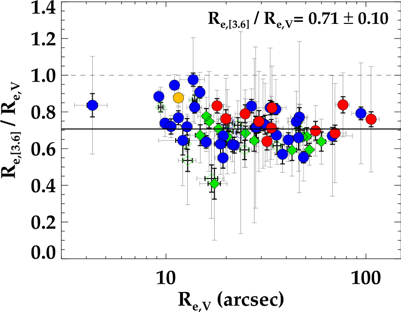
Figure 3: Ratio between $R_{\rm e,V}$ and $R_{\rm e,[3.6]}$ for our sample of galaxies. The solid thick line shows the average ratio ($R_{\rm e,[3.6]}$/$R_{\rm e,V}$). The dashed line marks the one-to-one relation. Circles denote E/S0 galaxies, diamonds Sa galaxies. Filled symbols indicate galaxies with good distance estimates, open symbols those with only recession velocity determinations. In blue we highlight Fast Rotators, in red Slow Rotators and in green the Sa galaxies. The special case of NGC 4550, with two similarly-massive counter-rotating disc-like components, is marked in yellow. Black/gray error bars denote the minimum/maximum uncertainties in our analysis (see §4.1)

The total apparent magnitude and corresponding uncertainty follows from $L_{\rm e}$, simply as $m=-2.5\log(2L_{\rm e})$. The mean effective surface brightness was computed by dividing $L_{\rm e}$, the total luminosity measured within one effective radius, by the area of the aperture, $A_{\rm e}=\pi$$R_{\rm e}$², and expressing it in magnitudes, $\langle\mu_{\rm e}\rangle$$=-2.5\log(L_{\rm e}/A_{\rm e})$. Since the effective luminosity and radius are correlated, the uncertainty in the mean effective surface brightness was derived after first computing the $\langle\mu_{\rm e}\rangle$ values for each of the corresponding Monte Carlo realisations of $L_{\rm e}$ and $R_{\rm e}$.

As already shown by other authors (e.g. Pahre, 1999; Bernardi et al., 2003; MacArthur et al., 2003; La Barbera et al., 2004), $R_{\rm e}$ values in the infrared appear to be, in general, smaller than those in optical bands. This is mostly due to the fact that galaxies tend to be bluer in the outer parts and therefore emit less light at these longer wavelengths (Peletier et al., 1990). In Figure 3 we show the relation we find between the independently measured $R_{\rm e,V}$ and $R_{\rm e,[3.6]}$ values; $R_{\rm e,[3.6]}$ is on average 29% smaller than $R_{\rm e,V}$. As a results of this, and as shown in § 6 and 7, differences are thus found in the scaling relations for the two photometric bands.

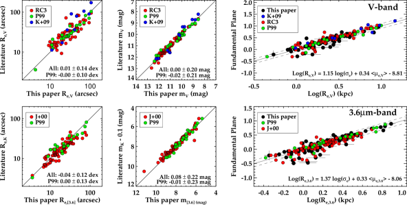
Figure 4: Comparison of our aperture photometry with the literature. Four leftmost panels: $R_{\rm e}$ and apparent magnitudes from this paper are compared to those in the literature (RC3, de Vaucouleurs et al. 1991; P99, Pahre 1999; J+00, Jarrett et al. 2000; K+09, Kormendy et al. 2009) for $V$- and $3.6\mu$m-bands. We subtracted 0.1 mag to the literature $K$-band values (i.e. the mean $K-$[3.6] colour for old stellar populations) to compensate for the colour difference. Mean offset and scatter are indicated for all sources (All) and P99 alone (as it is the only sample available in the two bands for the two quantities). Two rightmost panels: the best Fundamental Plane relations derived in § 7.1 showing our data as well as the literature data for our sample of galaxies (see details in § 4.2). Dashed lines in the Fundamental Plane relations mark the $1\sigma$ uncertainty.

4.2 Literature comparison

In order to test the reliability of our measurements, we have compared them with published values in the literature. This exercise can reveal large differences among sources, mainly depending on the depth of the data, photometric band and most importantly the methodology used to derive the relevant quantities. In Figure 4 we show the comparison of our estimated values with a few references in the literature (de Vaucouleurs et al., 1991; Pahre, 1999; Jarrett et al., 2000; Kormendy et al., 2009). When necessary, the literature major-axis $R_{\rm e}$ estimates have been transformed to geometric-mean radius to compare with our values obtained from circular apertures. As shown in the figure, the agreement with the different sources is generally good with a typical scatter of about 0.14 dex in $R_{\rm e}$ and 0.2 mag in apparent magnitude. The most notorious difference in our sample is that of NGC 4486 (M87), where our measured value in the $V$-band of $106\arcsec$, contrasts with other values in the literature ($95\arcsec$, de Vaucouleurs et al. 1991; $104\arcsec$, Pahre 1999; $171\arcsec$, Ferrarese et al. 1994; $194\arcsec$, Kormendy et al. 2009).

In addition, we show the best-fitting FP relations presented in § 7.1, including data from the same sources. We carry out this comparison to assess whether different methods to estimate the structural parameters can affect our relations. In order to minimize uncertainties, we have re-derived $\sigma_{\rm e}$ for each source’s $R_{\rm e}$ value. In addition, if not provided, our estimated distances were used to convert $R_{\rm e}$ from arcsec to kiloparsecs. In the case of Kormendy et al. (2009), we do not use their tabulated mean surface brightnesses, but instead compute them ourselves from the total luminosity and effective radii they provide in their Table 1 (columns 9 and 17). This is to mimic as much as possible our procedure to compute the photometric quantities. The figure shows that even though the structural parameters individually might vary among the different sources, in combination they agree well within the observed scatter, and thus our best-fitting parameters should not be biased in any particular way.

4.3 $V-[3.6]$ colours

Colour measurements have been widely used in the past to extract first order information on the stellar content of galaxies and constraint different formation scenarios (e.g. White, 1980; Carlberg, 1984). Here we determine the effective colour

$$(V-[3.6])_{\rm e}=-2.5\log(L_{V}(<R_{{\rm e},V})/L_{\rm[3.6]}(<R_{{\rm e},V}))+{\rm const.}$$ (4)

measured within a $R_{\rm e,V}$ aperture. The choice of $R_{\rm e,V}$ was preferred over $R_{\rm e,[3.6]}$ to match the aperture used to extract our SAURON spectroscopic quantities (see § 5). Aperture corrections, as devised in the IRAC Instrument Handbook, have been taken into account when deriving the colours. We will use the information from these parameters, together with absorption line-strength indices, to establish the stellar population properties of our galaxies in different regions of the scaling relations presented here.

Central colours (e.g. within $R_{\rm e,V}$/8) were not derived due to the complexity in matching the MDM and Spitzer PSFs. Furthermore, $V-[3.6]$ colour gradients were also discarded given the presence of dust in many of our galaxies, which introduces features in the colour profiles that cannot be accounted for with a single linear relation. Nevertheless, an in-depth analysis of colour profiles in the SAURON sample, using the Spitzer/IRAC $3.6$ and $4.5\mu$m bands, will be the subject of study in Peletier et al. (2011, in preparation).

5 SAURON QUANTITIES

In addition to the aperture photometry extracted from the MDM and Spitzer/IRAC images, we have determined a number of quantities from our SAURON integral-field data that are key for the analysis presented in this paper. These are parameters describing the richness in dynamical substructures and the stellar content of the galaxies in our sample. They have been computed following the procedures detailed in previous papers of the SAURON survey. Here we will briefly summarise the main aspects and refer the reader to the relevant papers for a full description of the methods employed. For convenience, the final set of spectroscopic quantities is listed in Tables 4 and  5.

5.1 Kinematic quantities

The stellar kinematics of our sample galaxies have been extracted following the procedure outlined in Papers IX and X. Briefly, we used pPXF (Cappellari & Emsellem, 2004) to fit a linear combination of stellar templates from the MILES library (Sánchez-Blázquez et al., 2006) and derive the best mean velocity $V$ and velocity dispersion $\sigma$ for each spectrum in our datacubes. In this paper we are mostly interested in extracting the true first two velocity moments of the line-of-sight velocity distribution (LOSVD), and therefore we deliberately do not fit the higher order moments ($h_{3}$, $h_{4}$). We use the extracted $V$ and $\sigma$ maps to compute $\lambda_{\rm R}$, a parameter that measures the specific angular momentum within $R_{\rm e,V}$ and that has led to the new kinematical classification of galaxies presented in Paper IX. Throughout this paper we will identify as Slow Rotators (hereafter SR) those galaxies with $\lambda_{\rm R}$$\leq 0.1$, and as Fast Rotators (hereafter FR) the rest (as all the papers in the SAURON series since Paper IX). We note that for this sample, the notation is consistent with that based on the improved criterion defined in Emsellem et al. (2011) for the galaxies in the ATLAS^3D sample (Cappellari et al., 2011).

In order to plot some of the scaling relations in § 6, we have measured the mean stellar velocity dispersion within an $R_{\rm e,V}$ aperture. For that purpose, we summed up all the spectra available within such a circular aperture and then computed $\sigma$ following the same procedure described above. Whenever the aperture was not fully contained within the SAURON FoV, we used the velocity dispersion calibration of Paper IV (equation 1) to correct our values. For some aspects in § 7.5, we have also measured the mean stellar velocity dispersion within an $R_{\rm e,V}$/8 aperture ($\sigma_{\rm{e},8}$). As in other papers in the survey (see Papers IV and XVII), we adopt a random error of 5% for our measured velocity dispersion values.

Finally, we make use of the results in Krajnović et al. (2008, hereafter Paper XII) to describe the level of kinematic substructure present in our maps (e.g. inner discs, kinematically decoupled cores, kinematic twists).

5.2 Stellar population quantities

As well as stellar kinematic quantities, we have also measured line-strength indices within $R_{\rm e,V}$. In this paper, in order to be fully consistent with the procedures employed to derive the stellar kinematics and to minimize the uncertainties in the absolute calibration of the line-strength indices, we have opted to measure the indices in the recently defined Line Index System (LIS) LIS-14.0 Å (Vazdekis et al., 2010, hereafter VAZ10). This method has the advantage of circumventing the use of the so-called Lick fitting functions for the model predictions, which requires the determination of often uncertain offsets to account for differences in the flux calibration between models and observations. The only required step to bring our flux-calibrated data to the LIS-14.0 Å system is to convolve the aperture spectra to a total FWHM of 14.0 Å. The choice of LIS-14.0 Å over other proposed systems (e.g. LIS-5.0 Å or LIS-8.4 Å) is imposed by the galaxy with the largest $\sigma_{\rm e}$ in our sample (i.e. NGC 4486).

Besides the standard Lick indices (Worthey, 1994) that can be measured within our wavelength range (i.e. H$\beta$, Fe5015, Mg$b$), we have also measured the H$\beta_{\rm o}$ index presented in Cervantes & Vazdekis (2009). This new index is similar to the classical H$\beta$ index, but it has the advantage of being less sensitive to metallicity. For convenience, we show the relation between the two indices for our galaxies in Fig. 5. We however warn the reader that this relation is necessarily biased by our sample selection. Since we are using stellar population models with solar abundance ratios, we use the [MgFe50]^′ index to minimise the effects of $\alpha$-elements over abundances (see Paper XVII). For galaxies with $R_{\rm e,V}$ larger than the SAURON coverage, we applied the line-strength aperture corrections devised in Paper VI. As established in Paper XVII, typical random errors for our measured values are 0.1 Å, with systematic uncertainties being 0.06, 0.15 and 0.08 Å for H$\beta$, Fe5015 and Mg$b$ respectively. We assume the same aperture corrections and errors as H$\beta$ for the H$\beta_{\rm o}$ index.

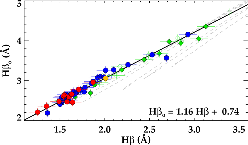
Figure 5: Relation between the H$\beta$ and H$\beta_{\rm o}$ line-strength indices for our sample galaxies. Colours and symbols as in Fig.3. The dashed gray lines mark the predictions of the Vazdekis et al. (2010) models for different metallicities. ([M/H]=[$-2.32,-1.71,-1.31,-0.71,-0.40,0.0,+0.2$]). Our sample appears to closely follow the predictions at high metallicities.

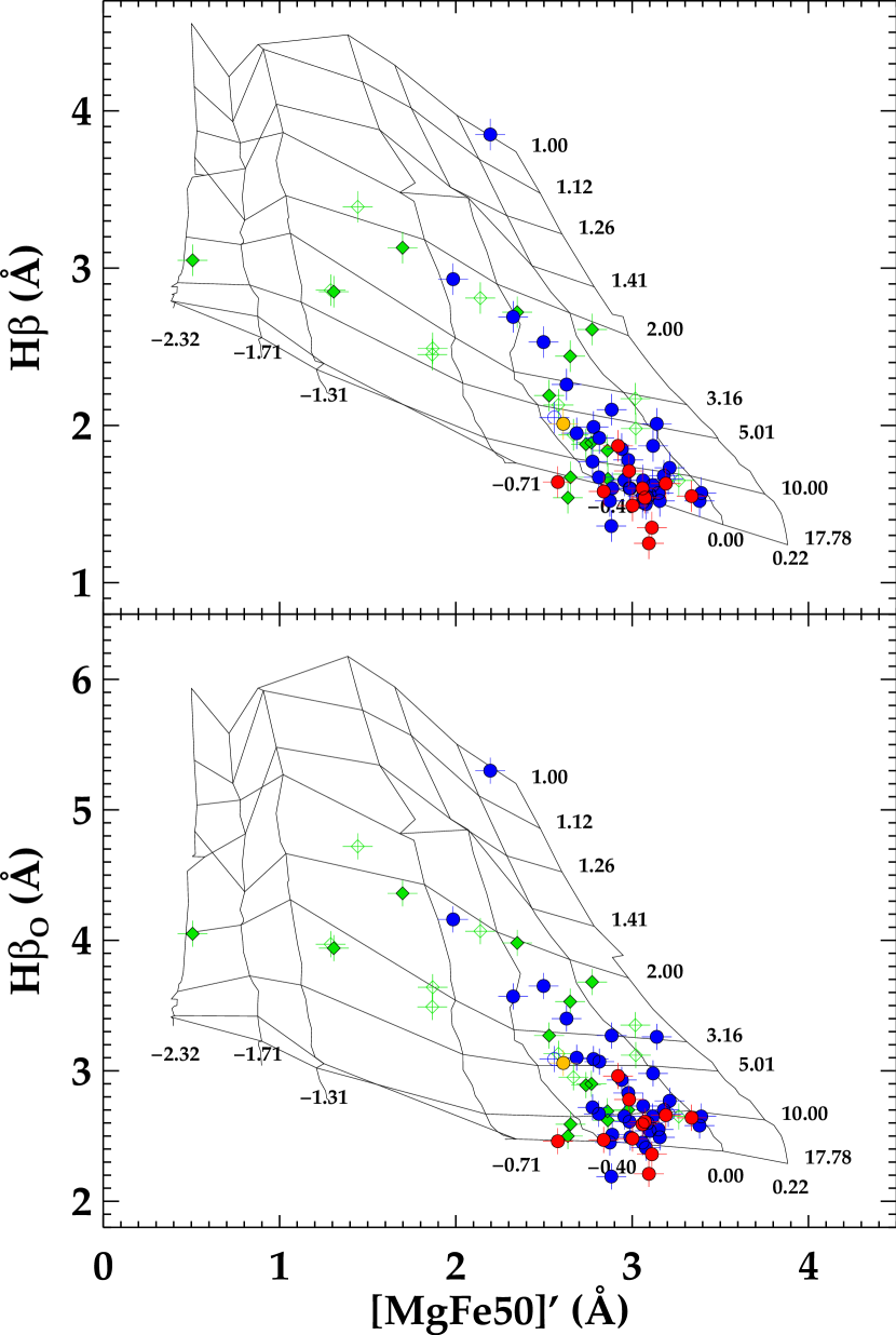
Figure 6: Line-strength index relations for the SAURON sample galaxies in the LIS-14.0 Å system (Vazdekis et al., 2010). Colours and symbols as in Fig. 3. The line-strength indices presented have been measured within a $R_{\rm e,V}$ aperture. Grids show model predictions for constant ages (horizontal lines with labels in Gyr) and metallicities (vertical lines labelled with [M/H] with respect to solar metallicity). The top panel shows the classical H$\beta$ Lick index (Worthey, 1994) versus [MgFe50]^′. The bottom panel shows the same diagram, but with the the recently defined H$\beta_{\rm o}$ index (Cervantes & Vazdekis, 2009) instead of H$\beta$.

Figure 6 shows the location of our galaxies in the H$\beta$ and H$\beta_{\rm o}$ vs [MgFe50]^′ diagrams in the LIS-14.0 Å system. The figure illustrates the main reasons for adopting the H$\beta_{\rm o}$ index over the traditional Lick H$\beta$ index: (1) the H$\beta_{\rm o}$ is more insensitive to metallicity than H$\beta$ down to [M/H]$\approx-0.71$, which makes the diagram more orthogonal, and (2) the vast majority of our galaxies fall within the model predictions, which is crucial for a proper estimation of the stellar mass-to-light ratios ($\gamma_{\ast}$).

Throughout this paper we investigate the potential dependencies on age via the line-strength index H$\beta_{\rm o}$. This is to be able to include the Sa galaxies in the same diagrams. While the use of ages, metallicities and abundance ratios is in general desired, estimates of these parameters from a single-stellar population (SSP) analysis, as was done for the 48 E and S0 galaxies in Paper XVII, are not recommended given the more continuous star-formation activity they have experienced (see Paper XI for more details on these and other caveats). The use of the H$\beta_{\rm o}$ index will instead provide a robust first order indication of the presence of young stars in our galaxies.

As is required in some of the relations we are presenting in this paper, we have estimated the $\gamma_{\ast}$ of our sample galaxies in both the $V$- and $3.6\mu$m-bands. We dedicate Appendices A and B to the description of the set of models and the methods used to derive these values.

6 SCALING RELATIONS

In this section we show some of the classic scaling relations for the SAURON sample of early-type galaxies. Although much work has been devoted to these relations in the literature, mostly separating galaxies by their morphological classification, here we will focus on how deviations from scaling relations depend on the kinematic information and stellar populations from our integral-field data. Since we found no significant correlation with the level of kinematic substructure or environment in any of the considered scaling relations (demonstrated in Appendix C), we focus on differences between the SR E/S0, FR E/S0, and Sa galaxies.

In the following sections we derive linear fits of the form $y=\alpha\,x+\beta$ to all relations, except the Fundamental Plane in § 7. We started from the fitexy routine taken from the IDL Astro-Library (Landsman, 1993) which fits a straight line to data with errors in both directions, which we extended to include possible correlations between the errors in both directions. To find the straight line that best fits a set of $N$ data points $x_{j}$ and $y_{j}$, with symmetric errors $\Delta x_{j}$ and $\Delta y_{j}$ and covariance $\mathrm{Cov}(x_{j},y_{j})$, the routine minimizes

$$\chi^{2}=\sum_{j=1}^{N}\frac{(y_{j}-\alpha\,x_{j}-\beta)^{2}}{\Delta_{\mathrm{obs},j}^{2}+\Delta_{\mathrm{int}}^{2}},$$ (5)

where the combined observational error is given by

$$\Delta_{\mathrm{obs},j}^{2}=(\Delta y_{j})^{2}+\alpha^{2}(\Delta x_{j})^{2}-2\,\alpha\,\mathrm{Cov}(x_{j},y_{j}),$$ (6)

and $\Delta_{\mathrm{int}}$ is the intrinsic scatter, which is increased until the value of $\chi^{2}$ per degrees of freedom is unity. Next, finding the changes in $\alpha$ and $\beta$ needed to increase $\chi^{2}$ by unity, yields the (1-$\sigma$) uncertainties on the best-fit parameters. The values of $x_{j}$ are normalized by subtracting the corresponding observational quantities per galaxy by the median value of all galaxies. This choice for the reference value (or pivot point) minimizes the uncertainty in the fitted slope $\alpha$ and its correlation with the intercept $\beta$. The details and benefits of this approach are described in Tremaine et al. (2002).

In deriving the errors $\Delta x_{j}$ and $\Delta y_{j}$, we include the uncertainties in all contributing quantities, i.e., the errors in the distances, the photometric quantities, the kinematic quantities (stellar velocity dispersion) and the stellar population quantities. Correlations in the photometric quantities are taking into account via our Monte Carlo realizations of § 4.1); for example, when deriving the error in $\langle\mu_{\rm e}\rangle$$=-2.5\log\left[L_{\rm e}/(\pi R_{\rm e}^{2})\right]$, we first compute from all realizations of $L_{\rm e}$ and $R_{\rm e}$ the corresponding $\langle\mu_{\rm e}\rangle$ values, and then derive the error as the (biweight) standard deviation. Similar Monte Carlo simulations of all quantities are used to calculate the covariance $\mathrm{Cov}(x_{j},y_{j})$, which can be significant especially when the same quantities are used in both $x_{j}$ and $y_{j}$, such as $R_{\rm e}$ in the Kormendy relation and the distance in the size-Luminosity relation.

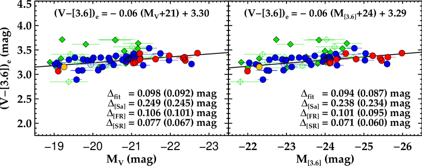
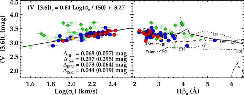
Figure 7: Colour-magnitude, colour-$\sigma_{\rm e}$, and colour-H$\beta_{\rm o}$ relations for the SAURON sample of galaxies. The best-fit linear relations to the E/S0 galaxies with good distance determinations are indicated in each panel and are shown with solid black lines. $\Delta_{\rm fit}$ indicates the observed and intrinsic scatters (the latter in parentheses) for the galaxies used to obtain the fit, while $\Delta_{[\dots]}$ represent the measured values for the different families around the best-fit relations. Colours and symbols as in Figure 3. The lines in the bottom-right panel correspond to the Marigo et al. (2008) model colour predictions combined with MILES (Vazdekis et al., 2010) Lick/IDS line-strength indices for different metallicities (see § 6.1 for details): [M/H]=[$-0.71$ (dotted-dashed), $-0.40$ (dashed), $0.00$ (solid), $+0.20$ (dotted)]. For reference, some ages (in Gyr) are indicated along the different metallicity tracks. Peaks seen in the colour tracks are due to an enhancement in the production rate of AGB stars, that causes a transient red phase in the integrated SSP colours (see Girardi & Bertelli, 1998).

Unless mentioned otherwise, for consistency and hence for easy comparison with most publications on scaling relations for early-type galaxies, only E/S0 galaxies with reliable distance estimates are included in the fits (i.e. 46 objects). The resulting best-fit relations are written in the figures themselves, while the best-fit parameters and corresponding errors are given in Table 1. The values indicated by $\Delta_{\mathrm{fit}}$ represent the scatter around the best-fit relation in the vertical direction, i.e., the (biweight) standard deviation of $y_{j}-\alpha\,x_{j}-\beta$, for the galaxies $j$ used in the fit. The value in parentheses is the intrinsic scatter, after subtracting, in quadrature, from $\Delta_{\mathrm{fit}}$ the (biweight) mean of the combined observational errors $\Delta_{\mathrm{obs,j}}$, which, as indicated in equation (6), include potential covariances between the variables. The intrinsic scatter values and corresponding error estimates can be found in Table 1. We confirmed that well within these errors, the intrinsic scatter values are the same as $\Delta_{\mathrm{int}}$ in equation 5 when the value of $\chi^{2}$ per degrees of freedom is unity. The other quoted scatter values $\Delta_{[\dots]}$ are based on all galaxies within the family/families indicated by the index in square brackets, i.e., also the galaxies with distances based on their recession velocities.

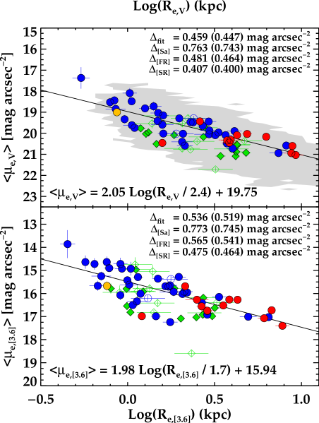
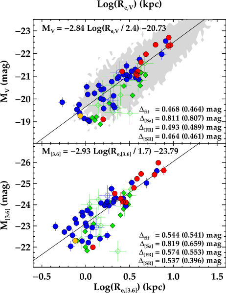
Figure 8: Kormendy (KR) and size-luminosity (SLR) relations for the galaxies in the SAURON sample in the $V$- and $3.6\mu$m-bands. Symbols as in Fig. 3. The thick solid line is the best fit relation (as indicated in the equation in each panel). $\Delta_{\rm fit}$ indicates the observed and intrinsic scatters (the latter in parentheses) for the galaxies used to obtain the fit, while $\Delta_{[\dots]}$ represent the measured values for the different families around the best-fit relations. The grey area marks the extent of the Bernardi et al. (2003) sample.

6.1 Relations with colour

We presented a set of CMRs in different photometric bands in Papers XIII and XV. In both cases the most deviant objects were galaxies displaying widespread ongoing star formation. Here we bring a new element to these works by investigating the location of galaxies with distinct kinematic properties (e.g. SR/FR) in the CMR.

In Figure 7 (top panels) we plot the CMRs for our sample galaxies using the effective colour ($V-[3.6]$)_e. There are two main sources that can change the slope and increase the intrinsic scatter in these CMRs: young stellar populations and dust extinction. They have opposite effects. Young populations will, in principle, shift galaxies down from the relation (galaxies become bluer), while dust will make galaxies appear redder than their stellar populations. Our sample contains galaxies which clearly exhibit dust (most notably Sa galaxies). Since we have made no attempt to correct for internal extinction, the position of these galaxies in this CMR cannot be used to infer information about their stellar populations. The reddest objects (NGC 1056, NGC 2273, NGC 4220, NGC 4235 and NGC 5953) in the plotted relations are indeed Sa galaxies with very prominent dust lanes.

The bottom-left panel of Fig. 7 shows the colour versus $\sigma_{\rm e}$ relation. Here both the FR and SR families define a much tighter sequence than in the CMRs shown in the top panels. Particularly striking are the relations defined by the SRs and FRs, with intrinsic scatters of only 0.019 and 0.064 mag respectively, as opposed to the Sa galaxies with deviations of about 0.30 mag, similar to those of the CMRs. The Sa galaxies systematically populate a region above the best-fit relation. Given the relative insensitivity of $\sigma_{\rm e}$ to dust (at least much less than absolute magnitudes in the optical), this diagram is potentially useful to remove dusty objects in samples destined for CMR studies. It also confirms that the average dust content is larger in spiral galaxies than in earlier-type systems. Despite these deviant objects, it is worth noting that there are a few Sa galaxies in the region populated by SR/FR galaxies.

As already shown in Papers XI, XIII and XV, our sample contains a number of objects with clear signs of widespread star formation (NGC 3032, NGC 3156, NGC 4150, NGC 3489, NGC 4369, NGC 4383, NGC 4405 and NGC 5953). Following the arguments outlined above, one might expect these galaxies to display the bluest colours (in the absence of dust). Surprisingly, this is not the case. In order to understand this behaviour, we have plotted in the bottom-right panel of Fig. 7 the effective colour versus the H$\beta_{\rm o}$ index measured within the same aperture. In addition to our data points, we also include colour predictions from Marigo et al. (2008, hereafter MAR08) together with line-strength predictions from the recently released MILES models (VAZ10). This combination of colours and line indices is consistent, in the sense that both predictions are based on the same set of isochrones (Girardi et al., 2000) and were computed for a Kroupa (2001) initial mass function. These isochrones take into account the latest stages of stellar evolution through the thermally pulsing asymptotic giant branch (AGB) regime to the point of complete envelope ejection. These models show that the dependence of the ($V-[3.6]$)_e colour with age is rather subtle even for young stellar populations, being much more sensitive to metallicity than age. This is the reason behind the lack of a strong signature of the youngest objects in the CMRs of Figure 7.

Now that we have assessed that metallicity is the main driver of the ($V-[3.6]$)_e colour, we can deduce from the colour-$\sigma_{\rm e}$ relation that there must be a strong correlation between metallicity and $\sigma_{\rm e}$. We have made an attempt to determine this relation by computing the best linear relation between metallicity ($[M/H]$) and $V-[3.6]$ colour in the MAR08 models ($V-[3.6]=0.73[M/H]+3.28$, see Appendix A), and then substituting that in the colour - $\sigma_{\rm e}$ relation found here. The selected galaxies are predominantly old and thus are well reproduced by single stellar population models. This yields a relation of the form

$$[M/H]=0.88\,(\pm 0.07)\log(\sigma_{\rm e})-1.92\,(\pm 0.16).$$ (7)

A similarly strong correlation was presented in Paper XVII ($[Z/H]($$R_{\rm e}$$)=0.32\log($$\sigma_{\rm e}$$)-0.82$) from an independent set of model predictions (Schiavon, 2007) and methodology (i.e. using line-strength indices rather than colours). Note, however, that the two relations cannot be directly compared as the one presented in Paper XVII is based on non-solar scaled stellar population models, while the one derived here is not. In order to compare them we have determined the metallicity of our models using the relation from the MAR08 models and then adjusted it assuming $[Z/H]=[M/H]+0.75[\alpha/$Fe$]$, where the factor 0.75 is a constant that depends on the element partition used for the models (R. Schiavon, private communication) and $[\alpha/$Fe$]$ is taken from Paper XVII. The slope of the resulting relation still appears to be a factor of 2 steeper than that of Paper XVII. The apparent inconsistency between the two determinations might indicate some issues in the modelling of the always complex AGB phase. The comparison with other relations in the literature (e.g. Jørgensen, 1999; Kuntschner, 2000; Trager et al., 2000; Thomas et al., 2005; Sánchez-Blázquez et al., 2006; Proctor et al., 2008; Allanson et al., 2009; Graves et al., 2009) is not straightforward either since, in addition to the stellar population models used, they are mostly based on central aperture measurements (both metallicity and velocity dispersion).

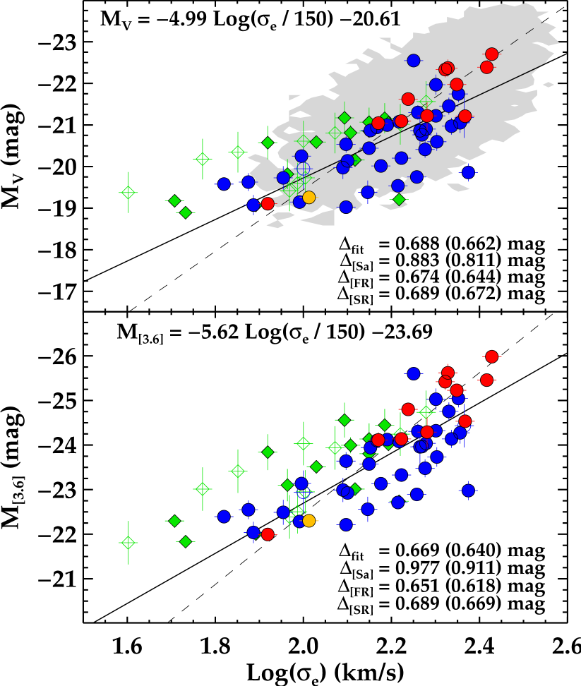
Figure 9: Faber-Jackson relation for the galaxies in the SAURON sample in the $V$- and $3.6\mu$m-band. Symbols as in Fig. 3. The solid line is the best fit relation (as indicated in the equation on the top left in each panel). The dashed line shows the best fit to the SR family (e.g. predominantly old systems). $\Delta_{\rm fit}$ indicates the observed and intrinsic scatters (the latter in parentheses) for the galaxies used to obtain the fit, while $\Delta_{[\dots]}$ represent the measured values for the different families around the best-fit relations. The grey area marks the extent of the Bernardi et al. (2003) sample.

6.2 Kormendy and size-luminosity relations

The KR and SLR for the SAURON sample of galaxies are shown together in Fig. 8. As already noticed by other authors, the value one obtains for these relations critically depends on the adopted selection criteria. In particular, the Malmquist bias caused by selecting galaxies according to their luminosities can have a large impact on the resulting best-fit relation (Nigoche-Netro et al., 2008). The volume and luminosity range of our survey means we lack small, high surface brightness, faint objects (as estimated from a comparison with the parent sample of galaxies in the ATLAS^3D survey, Cappellari et al., 2011). Nonetheless, limiting our fit to galaxies with distances below 25 Mpc (where our sample does not suffer those limitations) results in best-fit relations that are identical within the uncertainties. The comparison of our data in the KR and SLR with that of B03 shows that the strongest bias introduced in our analysis by the sample selection is in mean surface brightness. With the exception of NGC 5845 (the galaxy with the smallest $R_{\rm e}$), our galaxies seem to populate rather homogeneously the area defined by the B03 sample for $\langle\mu_{\rm e,V}\rangle$$\lesssim 21$ mag arcsec^-2. This implies a shallower KR and steeper SLR relation than in the more complete B03 sample.

The observed scatter around the best-fit relations is consistent with that found in others studies for galaxies within the same magnitude range (e.g. Nigoche-Netro et al., 2008). It appears that there is still a significant amount of intrinsic scatter in both relations, with the SR family displaying the smallest values. SR galaxies tend to populate the high luminosity end (with the exception of NGC 4458), while FR extend across the whole luminosity range displayed by our sample. In general, Sa galaxies appear to be fainter (by $\approx$0.8 mag) than SR/FR galaxies of the same size. This result is consistent with the observed strong dependence of these relations on morphological type (e.g. Courteau et al., 2007).

One interesting feature is the lack of large, high surface brightness (or small and very luminous) galaxies. This zone of avoidance (ZOA) was already noted by Bender et al. (1992) and has been later better defined by D’Onofrio et al. (2006) and Cappellari et al. (2011).

6.3 Faber-Jackson relation

In Figure 9, we show FJRs for our sample. As in previous relations, the SR family tends to occupy the high luminosity end of the relations. Sa galaxies, however, deviate from the best-fit relations in the sense that they systematically populate high luminosities for a given $\sigma_{\rm e}$ (for $\sigma_{\rm e}$$\lesssim$125 $\mbox{km s}^{-1}$). Disc galaxies are often characterised by the Tully-Fisher relation (Tully & Fisher, 1977) instead of the FJR. This is because in low mass systems the maximum rotational velocity is a much better tracer of total mass than the traditionally measured central velocity dispersions. The use of a large aperture for the velocity dispersion measurement ($\sigma_{\rm e}$) presented here significantly helps to improve matters by using a parameter close to the integrated second moment (see Paper IV). We believe that the observed offset is mainly a stellar population effect, whereby Sa galaxies are on average younger (and thus have in general lower stellar mass-to-light ratios) than earlier types, as already discussed in the literature (e.g. Paper XI). This effect is further supported by the best-fitting relation for the SRs (e.g. predominantly old systems). As shown in the figure, the slope of the relation for the SRs is larger (dashed line) than the original fit and in better agreement with B03. Nevertheless, the number of SRs in our sample is rather limited and thus complete samples (e.g. ATLAS^3D survey) are required to confirm the observed trend.

The FJR for our sample appears to ’bend’ toward low $\sigma_{\rm e}$ values at low luminosities. There is a hint of this feature in the relations for the Coma Cluster by Bower et al. (1992) and Jørgensen et al. (1996), but it is somehow not seen in other relations in the literature based on much larger numbers of galaxies (e.g. B03, La Barbera et al. 2010). This might be because galaxies with low velocity dispersions are often removed from the samples. Irrespective of selection effects, the slopes derived here are slightly shallower than previously found (e.g. Pahre, 1999). In part this is because it is common to use central velocity dispersions, which will increasingly deviate from the values reported here (measured in a larger aperture) for larger galaxies, as the velocity dispersion gradients are steeper in the inner parts of larger galaxies.

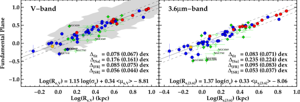
Figure 10: Edge-on views of the Fundamental Plane relation for the galaxies in the SAURON sample of galaxies in $V$- and $3.6\mu$m-bands. Symbols as in Fig. 3. The dashed lines mark the $1\sigma$ uncertainty (measured in log($R_{\rm e}$)) considering all objects. The solid line is the best fit relation (as indicated in the equation in each panel). $\Delta_{\rm fit}$ indicates the observed and intrinsic scatters (the latter in parentheses) measured along the log($R_{\rm e}$) axis for the galaxies used to obtain the fit, while $\Delta_{[\dots]}$ represent the measured values for the different families around the best-fit relations. The grey area marks the extent of the Bernardi et al. (2003) sample.

7 FUNDAMENTAL PLANE

In this paper we adopt the following notation for the FP:

$$\log(R_{\rm e})=\alpha\ \log(\sigma_{\rm e})+\beta\ \langle\mu_{\rm e}\rangle+\gamma.$$ (8)

The multivariate nature of the FP makes common least-squares minimisation algorithms not suitable to determine the main parameters ($\alpha,\beta,\gamma$). The literature is vast on alternative methods (e.g. Graham & Colless, 1997; La Barbera et al., 2000; Saglia et al., 2001), several of which we tested to yield consistent best-fit parameters within the corresponding estimated errors. The FP results presented in this paper are determined via an orthogonal fit by minimizing the sum of the absolute residuals perpendicular to the plane (e.g. Jørgensen et al., 1996). As in § 6, we include the uncertainties in all contributing quantities and take into account correlations in the photometric quantities via our Monte Carlo realizations.

In addition to the fitting scheme, sample selection biases in any of the quantities of Eq. 8 can have an important impact on the resulting coefficients (Nigoche-Netro et al., 2009). We have tested the sensitivity of our best-fit parameters to magnitude and distance (the two main selection criteria in our sample). Our sample is a good representation, in terms of luminosity, of the complete early-type galaxy population up to a distance of 25 Mpc, beyond which we lack small, faint, high surface brightness objects. Nevertheless, the inclusion of galaxies at larger distances hardly alters the best-fit parameters. In terms of luminosity alone, the best-fit parameters remain within the uncertainties as long as the faintest level in absolute magnitude is brighter than M${}_{\rm V}\approx-19$ and M${}_{\rm[3.6]}\approx-22$ magnitudes. Therefore, while distance has no major impact on the best-fit parameters, the removal of the fainter objects in our sample does. As shown in Fig. 7 of Hyde & Bernardi (2009), the expected bias in the $\alpha$ parameter due to our sample selection in terms of absolute magnitude is below 10%. As in other relations we restrict our fit to E/S0 galaxies with good distance determinations (i.e. filled SR/FR galaxies in the relations). From the comparison of our data with those of B03, we have established that the lack of objects with $\langle\mu_{\rm e,V}\rangle$$\lesssim 21.0$ mag arcsec^-2 in our sample effectively means that we miss galaxies with $R_{\rm e}$$\gtrsim$12 kpc. We have checked, using the B03 sample, that this effect does not seem to bias our results in any particular way.

7.1 Classic FP

In Figure 10 we present the FP for our sample galaxies in both the $V$-band and $3.6\mu$m-band. Sa galaxies share the same relation defined by early-type systems and are not clearly displaced below the relation as they usually are. We believe that the main reason for this behaviour is the way we have derived the quantities involved. When including spiral galaxies in the FP, it is customary to measure the photometric and spectroscopic quantities only within the bulge dominated region (e.g. Falcón-Barroso et al., 2002). Here we have measured the half-light radius, mean surface brightness and velocity dispersion in a consistent and homogeneous way for all galaxies regardless of morphological type. The importance of also computing the velocity dispersion within the same half-light radius was already shown in Figure 4: even though the photometric quantities taken from different literature sources for galaxies in our sample individually might vary substantially, when combined with a consistently measured integrated velocity dispersion, they all fall on our best-fit classic FP. In § 7.5 we investigate the effects in the best-fitting parameters if non-consistent velocity dispersion measurements are used.

The best-fit coefficients in both bands are somewhat inconsistent with some of the most recent works in the literature (e.g. Pahre, 1999; Bernardi et al., 2003; Proctor et al., 2008; Hyde & Bernardi, 2009; La Barbera et al., 2009). Although difficult to assess accurately, we believe that the main differences are due to a combination of photometric bands employed, fitting methods, and specially sample selection (since we include the Sa galaxies, unlike previous works). There is nevertheless a large disparity in the literature regarding the value of the FP coefficients. There seems to be, however, a consensus on the fact that $\alpha$ changes gradually with photometric band (increasing with wavelength) while $\beta$ remains almost constant (e.g. Hyde & Bernardi, 2009). The relations derived here share that property. The parameters also deviate from the virial theorem predictions (i.e. $\alpha=2$ and $\beta=0.4$ in the notation used here), an effect known as the ’tilt’ of the FP. At first sight it might seem surprising that the $\beta$ coefficient in the $V$-band, more sensitive to young stellar populations than infrared bands, has a similar value to that in the $3.6\mu$m-band. It is important to remember, however, that the $\gamma$ parameter, while assumed constant, is in fact a function of the total mass-to-light ratio ($M/L$), which is not necessarily constant among galaxies. In fact this $M/L$ depends on the stellar populations, i.e., one can express the total $M/L$ as a function of the stellar mass-to-light ratio $\gamma_{\ast}$ and the relative fraction of luminous to dark matter. It seems that during the fitting process stellar population effects conspire to keep $\beta$ constant while affecting $\alpha$ and $\gamma$.

7.2 Outliers and residuals

Not all the galaxies in our sample appear to follow the main FP relation. NGC 4382 is a well-known shell galaxy (e.g. Kormendy et al., 2009) which must have suffered some recent interaction event. It contains a rather young nuclei (3.7 Gyr, see Paper XVII), it is the youngest of all the non-CO detected SAURON galaxies (Combes et al., 2007) and it also displays a prominent central velocity dispersion dip (see Paper III). NGC 1056, NGC 4369, NGC 4383, NGC 5953 and NGC 7742 are Sa galaxies that contain a significant fraction of young stars within $R_{\rm e}$ (see Paper XI). NGC 3489 is one of the few early-type galaxies with a strong starburst in the last 2 Gyr (see Paper XVII). NGC 7332 was already recognised as an outlier of the FP in the optical and near-IR bands by Falcón-Barroso et al. (2002). Although it shows signs of widespread young populations, it is not at the level of other early-type galaxies. Nevertheless, this object is peculiar in that it is rich in kinematic substructure (Falcón-Barroso et al., 2004) and might have suffered from a recent interaction with NGC 7339. Moreover, the presence of two gaseous counter-rotating discs (Plana & Boulesteix, 1996) suggests that this galaxy might not be in dynamical equilibrium. It is interesting to note that the object in our sample with the strongest presence of widespread young populations, NGC 3032, does not deviate at all from the best fits.

Individual inspection of the outliers to understand the reasons for their unusual location with respect to the main FP strongly suggests young stellar populations as a common factor. We investigate this further by exploring whether the residuals correlate with stellar population quantities, such as H$\beta_{\rm o}$ shown in Figure 11. A correlation with the H$\beta_{\rm o}$ index indeed exists in both bands. With the exception of NGC 3032 noted above, galaxies with young stellar populations are systematically located below the main relation. These residuals suggest that, while metallicity gradients may contribute to the scatter in the FP, young populations are the dominant factor.

7.3 Influence of discs

In order to disentangle the possible effects on the FP due to structural non-homology in galaxies from those due to young stellar populations, we have carried out a simple experiment illustrated in Figure 12. We have defined a mock early-type galaxy as a spheroid with a light profile described by a de Vaucouleurs’ law. By construction, we put this spheroid on a generic FP (black filled circle and solid line). In order to assess the impact of an additional disc component, we added exponential discs to the spheroid, with scale lengths of respectively 0.2, 0.5, 1.0, 1.5 and 2.0 times the $R_{\rm e}$ of the spheroid (circles, upward triangles, diamonds, downward triangles and squares, respectively). For reference, we note that the typical values are $\gtrsim 5$ for late-type galaxies (Balcells et al., 2007). Additionally, we set the light of the disc to be 0.2, 0.5, 1.0, 2.0 and 5.0 times the light of the spheroid (dark blue, cyan, green, red, and pink, respectively). We have analysed the growth curves of all these mock galaxies in the same way as the real galaxies presented in this paper. We have assumed the same $\sigma_{\rm e}$ for all mock galaxies as its value does not seem to depend on the Sérsic $n$ used in the growth curves of our real galaxies.

The figure shows that with an increase of the disc light fraction, the mock galaxies tend to deviate more and more from the original FP. This is expected as the increase of light will lead to higher surface brightnesses, which in turn will push the objects below the relation. It is interesting, however, that the deviations only seem significant when the light fraction of the disc relative to the bulge is above a factor 2, regardless of the size of the disc relative to the spheroid. We note the large excursions in the $R_{\rm e}$ and vertical directions for large disc light fractions. Figure 12 also shows the effect of a compact or extended disc relative to the underlying spheroid. Compact bright discs tend to shift the galaxies towards the left of the relation, while extended ones shift towards the right. It is important to realise that the presence of a disc has little influence on the end location of a galaxy, unless the disc is rather bright relative to the spheroid.

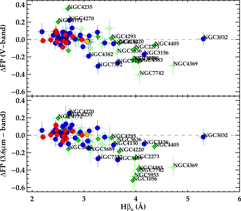
Figure 11: Residuals (along the log($R_{\rm e}$) axis) of the Fundamental Planes in Fig. 10 as a function of the H$\beta_{\rm o}$ line-strength index. Symbols as in Fig. 3.

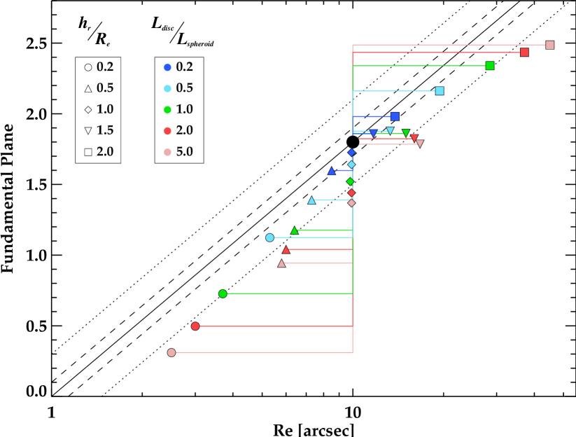
Figure 12: Simple experiment to show the effects of adding a disc to a spheroid on the location of galaxies in the FP (see § 7.3). The black dot marks the location of a pure spheroid, by construction on the FP. The black solid line marks the FP, and for reference dashed and dotted lines denote the 1$\sigma$ and 3$\sigma$ scatter in the relation shown in Figure 10. Different symbols indicate the ratio between the scale length of the added disc ($h_{r}$) and the effective radius ($R_{\rm e}$) of the underlying spheroid. Colours correspond to different fractions of disc light ($L_{\rm disc}$) relative to the spheroid ($L_{\rm spheroid}$).

There are, in principle, other sources for the scatter and tilt of the FP that we are not accounting for here in detail: projection effects, rotation, structural homology, etc. All those, besides stellar populations, have been studied in detail in the literature (e.g. Guzman et al., 1993; Saglia et al., 1993; Prugniel & Simien, 1994; Ciotti et al., 1996; Jørgensen et al., 1996; Graham & Colless, 1997; Prugniel & Simien, 1997; Pahre et al., 1998; Mobasher et al., 1999; Trujillo et al., 2004), although with different and sometimes conflicting conclusions. Recent studies, however, point to stellar populations and dark matter as the main drivers (Treu et al., 2006; Cappellari et al., 2006; Bolton et al., 2008; Graves & Faber, 2010). In this paper we focus on the effect of stellar populations only.

Results on the importance of young stellar populations in determining the location of galaxies in the FP were already highlighted in Paper XIII, based on GALEX observations in the ultraviolet regime. Although the analysis in that paper was limited to fewer galaxies than the sample presented here, it appears that an important fraction of the tilt and scatter of the UV FPs is due to the presence of young stars in preferentially low-mass early-type galaxies. Triggered by those results, we have attempted here to take a step further and correct the FP for stellar population effects in order to bring all galaxies into a common FP relation. The results of this exercise are shown in the following section.

7.4 FP corrected for stellar populations

A first test to assess the importance of young stellar populations on the tilt of the FP is to derive the best-fit relation after restricting the sample to predominantly old galaxies, i.e. SRs and FRs with H$\beta_{\rm o}$$\leq 3.0$ Å, and good distance determinations (35 objects). This simple experiment yields the best-fit parameters $\alpha=1.39$, $\beta=0.35$ and $\gamma=-9.61$ in the $V$-band and $\alpha=1.63$, $\beta=0.34$ and $\gamma=-8.85$ in the $3.6\mu$m-band. The dramatic change compared to Fig. 10 is the sudden increase of the $\alpha$ parameter, while $\beta$ remains almost unaltered. This object selection reduces the tilt of the FP and brings it much closer to the virial prediction. Nevertheless it is worth noting that the two $\alpha$ values (i.e. one for each band) are not close to each other, as one might expect if we had fully corrected for stellar population effects and hence were left with effects, in particular the luminous-to-dark matter fraction, that are insensitive to wavelength.

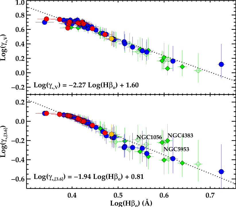
Figure 13: $\gamma_{\ast}$ vs H$\beta_{\rm o}$ relations for the SAURON sample galaxies in the $V$ and 3.6$\mu$m-band. Best-fitted (log-log) linear relations are indicated in each panel and plotted with a dotted line. $\gamma_{\ast}$ values have been determined as explained in Appendix B.

Considering the residuals in Fig. 11, one can take this experiment a step further and try to fully compensate for stellar populations (young and old) simultaneously. H$\beta_{\rm o}$ is not a quantity that directly enters the FP equation as defined in Eq. 8. However, as stated in Sect. 7.1, the $\gamma$ coefficient does depend on stellar populations via $\gamma_{\ast}$. We have made an attempt to estimate the effective $\gamma_{\ast}$ for each galaxy based on the combined MILES+MAR08 models, assuming a combination of two single stellar populations as the baseline star formation history (see Appendices A and B). The relations between our computed $\gamma_{\ast}$ and observed H$\beta_{\rm o}$ index are shown in Fig. 13, one for each photometric band. It appears that H$\beta_{\rm o}$ is strongly correlated with our measured $\gamma_{\ast}$ and thus could be used as a rough surrogate for $\gamma_{\ast}$. This behaviour was already shown in Paper IV for the H$\beta$ index. The fitted relations, despite being strong, have two important shortcomings: (1) they over-predict $\gamma_{\ast}$ at the low H$\beta_{\rm o}$ end and (2) they are rather uncertain for H$\beta_{\rm o}$ values above 3.0 Å. The first effect is an inherent limitation of the models used, i.e. any given set of models predicts a maximum $\gamma_{\ast}$ for a given initial mass function. The second effect is related to the wide range of allowed $\gamma_{\ast}$ for a given H$\beta_{\rm o}$ value, as parametrised by the set of two single stellar population models used here.

There are a few notable exceptions to the strong correlation at 3.6$\mu$m. These are objects located very close to the peaks of the $V-[3.6]$ colour in the MAR08 models for solar metallicities or above (i.e. NGC 1056, NGC 4383 and NGC 5953; see Fig. 7). Their H$\beta_{\rm o}$ values range from 3.8 to 4.2 Å. Since our $\gamma_{\ast,[3.6]}$ predictions are made after correcting for the colour difference with $\gamma_{\ast,V}$ (see Appendix A), it is not completely surprising that the $\gamma_{\ast,[3.6]}$ values in that region somehow deviate from the trend defined by neighbouring objects. However, sudden jumps in $\gamma_{\ast}$ of that magnitude seem unrealistic for these galaxies, and thus we opted to correct their values using the linear $\gamma_{\ast}$ vs H$\beta_{\rm o}$ relation in that band presented in Figure.13.

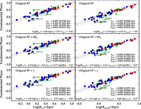
Figure 14: Edge-on views of the Fundamental Plane relations for the galaxies in the SAURON sample in the $V$- and $3.6\mu$m-band. Symbols as in Fig. 3. (Top row) Original FP relation. (Middle row) Original FP relation with a H$\beta_{\rm o}$ term. (Bottom row) Original FP relation with a $\gamma_{\ast}$ term. The dashed lines mark the $1\sigma$ uncertainty (measured along the log($R_{\rm e}$) axis) considering all objects. The solid line is the best fit relation (as indicated in the equation in each panel). $\Delta_{\rm fit}$ indicates the observed and intrinsic scatters (the latter in parentheses) measured along the log($R_{\rm e}$) axis for the galaxies used to obtain the fit, while $\Delta_{[\dots]}$ represent the measured values for the different families around the best-fit relations.

Figure 15: Edge-on views of the Fundamental Plane relations for the galaxies in the SAURON sample in the $V$- and $3.6\mu$m-band. Here $\sigma_{\rm e}$/8 ($\sigma_{\rm e,8}$) is used instead of $\sigma_{\rm e}$. Symbols as in Fig. 3. (Top row) Original FP relation. (Middle row) Original FP relation with a H$\beta_{\rm o}$ term. (Bottom row) Original FP relation with a $\gamma_{\ast}$ term. The dashed lines mark the $1\sigma$ uncertainty (measured in log($R_{\rm e}$)) considering all objects. The solid line is the best fit relation (as indicated in the equation in each panel). $\Delta_{\rm fit}$ indicates the observed and intrinsic scatters (the latter in parentheses) measured along the log($R_{\rm e}$) axis for the galaxies used to obtain the fit, while $\Delta_{[\dots]}$ represent the measured values for the different families around the best-fit relations.

Considering the nearly linear log-log relations between $\gamma_{\ast}$ and H$\beta_{\rm o}$, we can re-write the original FP equation in terms of these variables:

$$\log(R_{\rm e})=\alpha^{\prime}\log(\sigma_{\rm e})+\beta^{\prime}\langle\mu_{\rm e}\rangle+\gamma^{\prime}+\delta^{\prime}\log({\rm H}\beta_{o}),$$ (9)

$$\log(R_{\rm e})=\alpha^{\prime}\log(\sigma_{\rm e})+\beta^{\prime}\langle\mu_{\rm e}\rangle+\gamma^{\prime}+\delta^{\prime}\log(\gamma_{\ast}),$$ (10)

where $\gamma^{\prime}$ now depends (mainly) on the luminous-to-dark matter ratio.

In Figure 14 we plot the results of this experiment. In order to make a meaningful estimate of the effects of the stellar populations, we consider all objects with good distance estimates in the fit (60 galaxies, as opposed to the fits in Fig. 10 where only 46 E and S0 with good distances were considered). We perform this test in both bands. The top row in Fig. 14 shows the resulting fits using the classic FP definition (eq. 8), whereas the middle and bottom panels present the fits including the H$\beta_{\rm o}$ and $\gamma_{\ast}$ terms (equations 9 and 10). It seems that the inclusion of the Sa galaxies in the fits of the original FP relation (top panels) results in smaller slopes, which translates into larger departures from the virial expectations.

Our first attempt to bring deviant objects closer to the relation is to add the H$\beta_{\rm o}$ term in the FP relation. Unfortunately, leaving all the input parameters unconstrained results in very poor fits that, while successful in bringing back the most deviant galaxies, display much larger scatters than previous relations derived in this paper and, more importantly, have unreasonable coefficients. In order to get meaningful fits, we have instead fixed the H$\beta_{\rm o}$ terms to the coefficients expected from the fits to the original FP residuals versus H$\beta_{\rm o}$ shown in Fig. 11. The results of fixing this term are shown in the middle panels. These fits are able to bring the young objects much closer to the relations and at the same time to slightly reduce the intrinsic scatters. The $\alpha^{\prime}$ coefficients have increased with respect to the original relation, getting them a step closer to the virial prediction, while the $\beta^{\prime}$ values have only changed within the uncertainties ($\approx 0.01$). The main disadvantage of H$\beta_{\rm o}$ as a substitute to $\gamma_{\ast}$ can be seen in the case of NGC 3032. As already shown in Fig. 13, this galaxy is a deviant object in the $\gamma_{\ast}$ vs H$\beta_{\rm o}$ relation, and this translates in it being pushed out of the relation (its measured H$\beta_{\rm o}$ value over-predicts its true $\gamma_{\ast}$).

Finally, in the bottom panels of Figure 14, we add the $\gamma_{\ast}$ term in the FP relation. In this case the unconstrained fits result in physically meaningful coefficients, while at the same time bringing the most deviant points closer to the relation. The best-fit parameters reduce the FP tilt compared to the original relations by almost 50% in each band. It is important to remark that best-fit coefficients in both bands are now consistent within the errors, as expected if we had corrected for the effects of stellar populations. The coefficients, at least in the 3.6$\mu$m-band, are also within the uncertainties of those obtained by fitting the old galaxies only (see above). While in the $V$-band most of our young objects get closer to the relation, in the 3.6$\mu$m-band this is not the case (even though we have corrected their $\gamma_{\ast}$ estimates based on Fig. 13 as explained above). In fact, these objects cannot be brought back to the 3.6$\mu$m-band relation even with the most extreme $\gamma_{\ast}$ values allowed by our stellar population fitting procedure.

As an additional exercise (not shown here) we have studied the effect of using the ($V-[3.6]$)_e colour, instead of H$\beta_{\rm o}$ or $\gamma_{\ast}$, in reducing the tilt of the FP. As expected, given the poor sensitivity of this colour to age (as shown in Fig. 7), this quantity does not help reducing the tilt. At the same time it also demonstrates that metallicity cannot be a major player in producing the tilt (since this colour correlates strongly with metallicity, see Appendix A).

It is important to remind the reader that we have only corrected for the effects produced by stellar populations, and partly by rotation (by using $\sigma_{\rm e}$). Still there are a number of other factors that influence the final location of galaxies in the FP. The complex manner in which star formation and dust compensate each other might be at the heart of the location discrepancies of some of the objects in the $V$- and 3.6$\mu$m-band FPs. Nevertheless, the results of our exercise demonstrate that it is possible to correct for stellar population effects and bring most galaxies to a common relation, regardless of their morphological type and photometric band employed by including sensible estimates of the stellar mass-to-light ratios. This approach was previously adopted by Prugniel & Simien (1996) in a sample of elliptical galaxies and has been more recently exploited by other groups on much larger samples, though still restricting the analysis to early-type systems (e.g. Allanson et al., 2009; Hyde & Bernardi, 2009; Graves & Faber, 2010). Our results are largely consistent with those.

7.5 Scatter in the FP

One of the most striking features observed in our fits of the FP is the very tight relation defined by the SR galaxies in both bands. This is not a totally unexpected result as SR galaxies are uniformly old, but it is remarkable how the trend is kept even for smaller and fainter galaxies (as SR galaxies extend over the whole range in luminosity of our sample). The FR family displays slightly larger rms ($\Delta_{\rm[FR]}$) values. The scatter of the Sa galaxies appears to be the largest of the cases we have studied here. The different panels in Fig. 10 and 14 show the observed as well as the intrinsic scatter (within brackets) for each family. For easily comparison with other works in the literature we choose to provide them measured along the log($R_{\rm e}$) direction.

The first thing to notice for the classic fits in Fig. 10 and 14 is the differences between the values reported. The scatters for the Sa galaxies in the first figure are larger than in the second. Conversely the rms for the SR/FR families is smaller in the first figure than in the second one. This is simply due to the fact that for determining the FP we fit only the SR/FR galaxies in Fig. 10, while Fig. 14 includes the Sa galaxies as well. If we focus on this last figure we observe, apart from a change in the slopes, an improvement (i.e. a decrease) of the scatter for all families when we include the H$\beta_{\rm o}$ and $\gamma_{\ast}$ terms to correct for the effects of young populations. It is also interesting to note that once corrected for this effect, the intrinsic values found for the different families indicate that while FR and Sa galaxies are consistent within the uncertainties, they are clearly different from those of the SRs. This finding emphasises the results presented in Paper IX and subsequent papers in the SAURON series suggesting, based on our kinematic classification, that these may be intrinsically a different kind of galaxies. This clear distinction is not found between morphologically classified elliptical and lenticular galaxies.

The comparison of the scatter presented here with others in the literature has to be treated with caution as, while most works concentrate in E/S0 galaxies, the different samples were selected with very different criteria in terms of luminosity or velocity dispersion. In addition, the methods used to fit the relation can affect this comparison, although the minimisation of the residuals via an orthogonal fit is the most widely adopted. There is a general agreement that the observed scatter is consistent among photometric bands, a result we share. The typical observed scatter for a general population of E/S0 galaxies is around 0.10 dex in log($R_{\rm e}$) (e.g. Jørgensen et al., 1996; Pahre et al., 1998; Zibetti et al., 2002; La Barbera et al., 2010), with decreasing values ($\sim$0.07 dex) as soon as low velocity dispersion ($\sigma\lesssim 70$$\mbox{km s}^{-1}$) or fainter galaxies (M${}_{r}\gtrsim-23$ mag) are removed from their samples (e.g. Jørgensen et al., 1996; Bernardi et al., 2003; La Barbera et al., 2008; Gargiulo et al., 2009). The values measured here for the SR/FR are in good agreement with those in the literature for general samples of E/S0 galaxies. In the specific case of Jørgensen et al. (1996), the lowest observed scatter, 0.047 dex, is measured for galaxies with no presence of discs and M${}_{r}\lesssim-23.1$ mag. They report that this value is consistent with the measurement errors. The closest set of galaxies in our sample matching those constraints is the SR family. For this group, we find a very small amount of intrinsic scatter left, $0.021\pm 0.029$ dex and $0.012\pm 0.050$ dex in the V-band and 3.6mu-band respectively. The uncertainties in the our estimates suggest that the scatter around the best-fit FP are fully explained by the observational errors.

Another interesting point to discuss is whether the use of a large aperture velocity dispersion, instead of a central value, helps to reduce the intrinsic scatter in the relation. This was nicely discussed in Graham & Colless (1997) and Busarello et al. (1997), using samples of elliptical and lenticular galaxies and dynamical models with some assumptions on the shape of the velocity ellipsoid. The SAURON spectrograph gives us now the chance to repeat this exercise using real data. We have measured the velocity dispersion within $R_{\rm e,V}$/8 ($\sigma_{\rm e,8}$) for our sample of galaxies and then fit the FP in the same manner done in Fig. 14. This is presented in Fig. 15. The different panels show that the use of a small aperture velocity dispersion affects the resulting fits in two important ways: (1) increasing the intrinsic scatter of the relations for all families of objects, (2) the measured parameter $\alpha$ has lower values than those obtained when $\sigma_{\rm e}$ is used. The first point is mainly due to the fact that with the smaller aperture we are probing regions of the galaxies where intense star formation is taking place or inner discs exist, and thus the measured velocity dispersion is more representative of areas around the nuclei than the galaxy as a whole. The second effect is likely produced by the fact that $\sigma_{\rm e,8}$ systematically departs from $\sigma_{\rm e}$ (i.e. it is larger) for increasing $\sigma_{\rm e}$ values. This, together with the expected relation between $R_{\rm e}$ and $\sigma_{\rm e}$ (given the SLR and FJR), helps to reduce the measured slope of the FP relation. Overall, we estimate an increase of around 15% in the intrinsic scatter and an average 10% decrease in $\alpha$ as a result of using a central value for the velocity dispersion term. It is also worth noting that the scatter of the Sa galaxies has not increased as much as for the SR and FR families. This supports the idea that star formation in early-type systems takes place predominantly in their central regions, while for Sa galaxies this can happen over a much larger region (see also Paper XI), and therefore it does not necessarily make much difference to measure the velocity dispersion in a small or large aperture. Alternatively, this result could be due to the shallower nature of the stellar velocity dispersion profiles of the Sa galaxies compared to those of the SR/FR galaxies.

8 Conclusions

In this paper we report results from photometric follow-up conducted in the context of the SAURON project. We use ground-based MDM $V$-band and Spitzer/IRAC 3.6$\mu$m-band imaging to characterise our sample of E, S0 and Sa galaxies. We perform aperture photometry to derive homogeneous half-light radii, mean effective surface brightnesses and total magnitudes. Combined with the SAURON integral-field spectroscopic observations, this allows us to explore and understand the location of the galaxies in the main scaling relations as a function of the level of rotation, kinematic substructure, stellar populations and environment.

A number of conclusions can be derived from the work presented and are summarised in the following points:

• The level of kinematic substructure (as determined from our stellar kinematic maps) or the environment do not lead to a preferred location in any of the scaling relations investigated. However, this is subject to the potential biases introduced by our sample selection. Our cluster environment is defined by the Virgo Cluster and Leo group.

• The Slow Rotator (SR) galaxies define tighter relations than Fast Rotator (FR) galaxies. While this is not totally unexpected (i.e. SR are uniformly old systems), it is remarkable how the trend is kept both for small and large $R_{\rm e}$. We find that the SR and FR galaxies do not populate distinct locations in the scaling relations. The Sa family is the main contributor to the scatters.

• Sa galaxies deviate from the colour-magnitude and colour-$\sigma_{\rm e}$ relations due to the presence of dust. SR/FR galaxies instead define very tight relations.

• Surprisingly, extremely young objects do not display the bluest $(V-[3.6])$ colours of our sample, as is usually the case for optical colours. This can be understood in the context of the large contribution of TP-AGB stars to the infrared even for young populations, which makes the $(V-[3.6])$ colour almost insensitive to age for populations above $\approx 1$ Gyr. This effect results in a very tight $(V-[3.6])-$$\sigma_{\rm e}$ relation that allows us to define a strong correlation between metallicity and $\sigma_{\rm e}$.

• A large number of Sa galaxies appear to follow the main relations defined by earlier-type systems, and are not necessarily offset as previously found. We believe this is due to the use of $\sigma_{e}$ (the stellar velocity dispersion integrated within $R_{\rm e}$), which is not as much influenced by the presence of young inner discs and accounts to a large extent for rotation in the galaxies.

• FR and Sa galaxies that appear offset from the relations correspond mostly to objects with extremely young populations and signs of on-going, extended star formation (as already highlighted in Papers XIII and XV). For the specific case of the Fundamental Plane, we made an attempt to correct for this effect so that all galaxies are part of a tight, single relation. Once this is done, the FP coefficients in the $V$- and 3.6$\mu$m-bands are the same within the uncertainties. The new estimated coefficients suggest that differences in stellar populations account for about 50% of the observed tilt with respect to the virial prediction.

• The observed scatter of the SR family around the Fundamental Plane is smaller than that of the FR or Sa galaxies. After correcting for stellar populations, the SR family shows almost no intrinsic scatter around the best-fit Fundamental Plane.

• The use of a velocity dispersion within a small aperture (e.g. $R_{\rm e}$/8) in the Fundamental Plane results in an increase of around 15% in the intrinsic scatter and an average 10% decrease of the tilt away from the virial relation (as a result of the correlation between $R_{\rm e}$ and $\sigma_{\rm e}$, given by the size-luminosity and Faber-Jackson relations).

We have deliberately focused on the role of stellar populations on the main scaling relations of early-type galaxies. The effects other galaxy properties exert on them (e.g. non-homology, anisotropy and dark matter variations) will be studied in ongoing and upcoming integral-field spectroscopic surveys.

Table 1: Scaling relations best-fit parameters

Relation	Band	$\alpha$	$\beta$	$\gamma$	$\delta$	$\Delta_{\rm fit}$	$\Delta_{\rm[SR]}$	$\Delta_{\rm[FR]}$	$\Delta_{\rm[Sa]}$	N	Sample
(1)	(2)	(3)	(4)	(5)	(6)	(7)	(8)	(9)	(10)	(11)	(12)
Colour-magnitude	$V$	$-0.06\pm 0.02$	$3.30\pm 0.02$	-	-	$0.092\pm 0.010$	$0.067\pm 0.009$	$0.101\pm 0.011$	$0.245\pm 0.010$	46	E/S0
Colour-$\sigma_{\rm e}$	-	$0.64\pm 0.07$	$3.27\pm 0.01$	-	-	$0.057\pm 0.011$	$0.019\pm 0.017$	$0.064\pm 0.010$	$0.295\pm 0.010$	46	E/S0
Kormendy	$V$	$2.05\pm 0.22$	$19.75\pm 0.07$	-	-	$0.447\pm 0.061$	$0.400\pm 0.029$	$0.464\pm 0.072$	$0.743\pm 0.079$	46	E/S0
Size-luminosity	$V$	$-2.84\pm 0.22$	$-20.73\pm 0.07$	-	-	$0.464\pm 0.028$	$0.461\pm 0.026$	$0.489\pm 0.028$	$0.807\pm 0.040$	46	E/S0
Faber-Jackson	$V$	$-4.99\pm 0.71$	$-20.61\pm 0.11$	-	-	$0.662\pm 0.071$	$0.672\pm 0.057$	$0.644\pm 0.088$	$0.811\pm 0.193$	46	E/S0
Fund. Plane	$V$	$1.15\pm 0.05$	$0.34\pm 0.01$	$-8.81\pm 0.19$	-	$0.067\pm 0.015$	$0.044\pm 0.016$	$0.075\pm 0.017$	$0.161\pm 0.037$	46	E/S0
Fund. Plane	$V$	$1.08\pm 0.04$	$0.33\pm 0.01$	$-8.56\pm 0.18$	-	$0.078\pm 0.018$	$0.051\pm 0.015$	$0.070\pm 0.018$	$0.149\pm 0.038$	60	E/S0/Sa
Fund. Plane + H$\beta_{\rm o}$	$V$	$1.30\pm 0.04$	$0.32\pm 0.01$	$-9.22\pm 0.19$	$0.77$	$0.073\pm 0.016$	$0.043\pm 0.014$	$0.077\pm 0.016$	$0.116\pm 0.038$	60	E/S0/Sa
Fund. Plane + $\gamma_{\ast}$	$V$	$1.56\pm 0.13$	$0.32\pm 0.01$	$-9.03\pm 0.31$	$-0.55\pm 0.13$	$0.064\pm 0.031$	$0.021\pm 0.029$	$0.070\pm 0.029$	$0.088\pm 0.051$	60	E/S0/Sa
Colour-magnitude	[3.6]	$-0.06\pm 0.01$	$3.29\pm 0.01$	-	-	$0.087\pm 0.010$	$0.060\pm 0.010$	$0.095\pm 0.011$	$0.234\pm 0.010$	46	E/S0
Kormendy	[3.6]	$1.98\pm 0.27$	$15.94\pm 0.08$	-	-	$0.519\pm 0.082$	$0.464\pm 0.042$	$0.541\pm 0.085$	$0.745\pm 0.097$	46	E/S0
Size-luminosity	[3.6]	$-2.93\pm 0.26$	$-23.79\pm 0.08$	-	-	$0.541\pm 0.029$	$0.396\pm 0.024$	$0.553\pm 0.120$	$0.659\pm 0.128$	46	E/S0
Faber-Jackson	[3.6]	$-5.62\pm 0.69$	$-23.69\pm 0.10$	-	-	$0.640\pm 0.069$	$0.669\pm 0.054$	$0.618\pm 0.085$	$0.911\pm 0.187$	46	E/S0
Fund. Plane	[3.6]	$1.37\pm 0.05$	$0.33\pm 0.01$	$-8.06\pm 0.19$	-	$0.071\pm 0.014$	$0.037\pm 0.012$	$0.083\pm 0.017$	$0.224\pm 0.035$	46	E/S0
Fund. Plane	[3.6]	$1.23\pm 0.04$	$0.32\pm 0.01$	$-7.49\pm 0.16$	-	$0.099\pm 0.016$	$0.053\pm 0.012$	$0.084\pm 0.017$	$0.191\pm 0.036$	60	E/S0/Sa
Fund. Plane + H$\beta_{\rm o}$	[3.6]	$1.47\pm 0.04$	$0.31\pm 0.01$	$-8.35\pm 0.18$	$0.96$	$0.082\pm 0.014$	$0.044\pm 0.011$	$0.080\pm 0.015$	$0.132\pm 0.036$	60	E/S0/Sa
Fund. Plane + $\gamma_{\ast}$	[3.6]	$1.61\pm 0.12$	$0.32\pm 0.01$	$-8.39\pm 0.37$	$-0.60\pm 0.15$	$0.057\pm 0.041$	$0.012\pm 0.050$	$0.065\pm 0.036$	$0.096\pm 0.057$	60	E/S0/Sa

NOTES:
(1) We use the following notation for each of the scaling relations:
Colour-magnitude: ($V-[3.6]$)${}_{\rm e}=\alpha($M$+24)+\beta$ for the $V$-band and ($V-[3.6]$)${}_{\rm e}=\alpha($M$+21)+\beta$ for the 3.6$\mu$m-band
Colour-$\sigma_{\rm e}$: ($V-[3.6]$)${}_{\rm e}=\alpha\log($$\sigma_{\rm e}$$/\sigma_{\rm ref})+\beta$, with $\sigma_{\rm ref}=150$.
Kormendy relation: $\langle\mu_{\rm e}\rangle$$=\alpha\log($$R_{\rm e}$$/R_{\rm ref})+\beta$, with $R_{\rm ref}$ equal to $2.4$ and $1.7$ for the $V$- and 3.6$\mu$m-band respectively.
Size-luminosity: M $=\alpha\log($$R_{\rm e}$$/R_{\rm ref})+\beta$, with $R_{\rm ref}$ equal to $2.4$ and $1.7$ for the $V$- and 3.6$\mu$m-band respectively.
Faber-Jackson: M $=\alpha\log($$\sigma_{\rm e}$$/\sigma_{\rm ref})+\beta$, with $\sigma_{\rm ref}=150$.
Fundamental Plane: $\log($$R_{\rm e}$$)=\alpha\log($$\sigma_{\rm e}$$)+\beta$$\langle\mu_{\rm e}\rangle$$+\gamma$
Fundamental Plane + H$\beta_{\rm o}$: $\log($$R_{\rm e}$$)=\alpha\log($$\sigma_{\rm e}$$)+\beta$$\langle\mu_{\rm e}\rangle$$+\gamma+\delta\log($H$\beta_{\rm o}$$)$
Fundamental Plane + $\gamma_{\ast}$: $\log($$R_{\rm e}$$)=\alpha\log($$\sigma_{\rm e}$$)+\beta$$\langle\mu_{\rm e}\rangle$$+\gamma+\delta\log($$\gamma_{\ast}$$)$
Note that the $\delta$ parameter for the Fundamental Plane + H$\beta_{\rm o}$ term has been held fixed (see §7.4).
(2) Photometric band of the fit. (3-6) Best-fit parameters and uncertainties.
(7-10) Intrinsic scatter and uncertainties for the fit and SR/FR/Sa families. Values for the colour-magnitude, colour-$\sigma_{\rm e}$, size-luminosity and Faber-Jackson are expressed in magnitudes, while in mag arcsec^-2 for the Kormendy relation. For the Fundamental Plane, the intrinsic scatter is given in dex along the log($R_{\rm e}$) direction.
(11-12) Number of objects in the fit and type of galaxies fitted. Only galaxies with good distance estimations have been included in the fit.

Appendix A Stellar Population models

As described in Sect. 6.1, we use a combination of the new MILES models (VAZ10) together with those of MAR08 to interpret our results. The choice of these models is deliberate. The MILES models currently provide one of the best libraries for the study of stellar populations at optical wavelengths. They are based on the MILES stellar library (Sánchez-Blázquez et al., 2006) which consists of $\approx 1000$ stars spanning a large range in atmospheric parameters and covering the wavelength range 3525-7500Å at 2.3Å (FWHM) spectral resolution. The spectral resolution, spectral type coverage, flux calibration accuracy and number of stars represent a substantial improvement over previous libraries used in population synthesis models. The MAR08 models on the other hand provide colour predictions at infrared wavelengths, and in particular for the Spitzer/IRAC 3.6$\mu$m-band data used here. These models differ from MILES in that they have incorporated an improved treatment of the thermally-pulsing asymptotic giant branch (TP-AGB) phase. The main advantage is that both libraries make use of the same set of theoretical isochrones (Girardi et al., 2000) and therefore allow us to generate photometric and spectroscopic predictions on the same age and metallicity scales, as well as for the same type of initial mass function (IMF). For the purpose of our work we focus on predictions for a Kroupa IMF (not corrected for binaries). The spectroscopic measurements have been performed after transforming the MILES models to the LIS-14.0Å system (see VAZ10).

Although still somewhat controversial in the details, the importance of the TP-AGB phase on observed colours has been recognised (e.g. Maraston, 2005). In order to understand the impact the TP-AGB phase has on the optical and infrared colours used here, we show in Figure 16 the photometric predictions of both sets of models up to the reddest band predicted by the MILES models ($K$-band). Given the small difference observed between the $K$- and 3.6$\mu$m colours, any conclusion based on $K$-band can be extended to the Spitzer/IRAC 3.6$\mu$m data. The top row shows the $V-K$ colour as a function of age for a range of metallicities. The difference between the MILES and MAR08 models, at large metallicities in particular, is significant. While the MILES models predict a strong correlation between colour and age, this is essentially non-existent for ages above 1 Gyr in the MAR08 models (which show a constant behaviour). This result contrasts with the good agreement, albeit with a small offset, between the two sets of models for the $B-V$ colour (as shown in the middle panel) over the range of ages and metallicities displayed by our data. This is confirmed in the bottom panel, showing that the predicted $V$-band magnitudes in both set of models are consistent except for an offset.

Figure 16: Comparison of the colour and luminosity predictions of the Marigo et al. (2008) and MILES (Vazdekis et al., 2010) models as a function of age (in Gyr) and metallicity (increasing from $-2.32$ to $+0.22$, from bottom to top of the figures, with increasing colour or luminosity), for a Kroupa initial mass function.

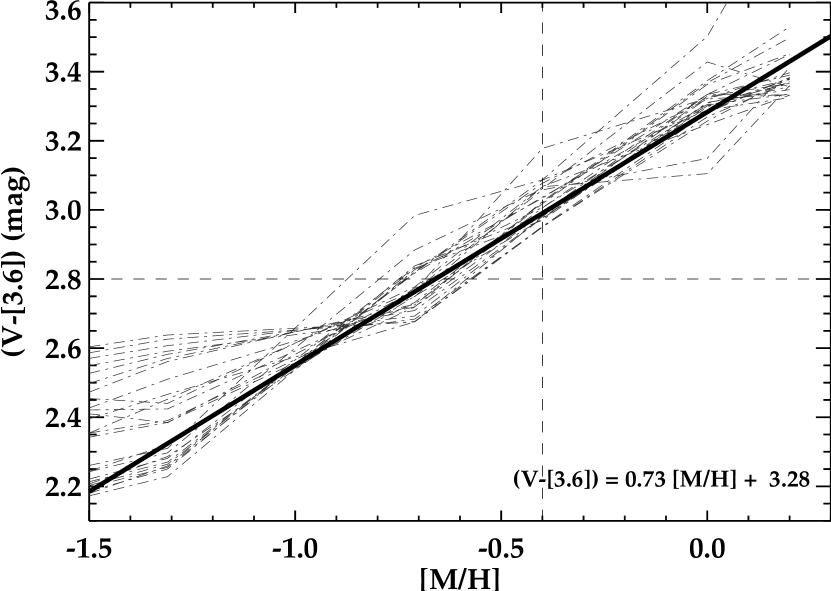
Figure 17: ($V-[3.6]$) vs metallicity relation from the single stellar population models of Marigo et al. (2008). Dashed lines mark the predictions for different ages and metallicities. The thick solid line shows the best fit for the range of colours and H$\beta_{\rm o}$ values defined by our sample (top-right quadrant delimited by the horizontal and vertical dashed lines). The fitted relation is also indicated.

The large similarities between the MILES and MAR08 models at optical wavelengths allow us to safely combine the spectroscopic prediction from MILES and the photometric ones from MAR08 (as shown in Fig. 7).

As shown in §6.1, our sample galaxies display a very tight correlation between the ($V-[3.6]$)_e colour and $\sigma_{\rm e}$. Transforming that relation into a mass-metallicity relation requires to derive a relation between the ($V-[3.6]$) and metallicity ($[M/H]$) first. This is shown in Fig. 17, based on the MAR08 models for the range of colours and H$\beta_{\rm o}$ values exhibited by our sample (($V-[3.6]$)${}_{\rm e}\geq 2.8$ mag and H$\beta_{\rm o}$$\leq$3.0Å).

Appendix B Stellar Mass-to-light ratios

The effective stellar mass-to-light ratio ($\gamma_{\ast}$) is one of the most sought after quantities when it comes to determine the stellar mass content or to derive the fraction of dark matter present in a galaxy (e.g. after comparison with dynamical estimates). Pioneering work relied on optical and infrared colours (e.g. Bell & de Jong, 2001). This has been extended over the years to provide new calibrations based on different sets of filters (Longhetti & Saracco, 2009; Zibetti et al., 2009). The use of full spectral fitting methods has also been extensive (e.g. Panter et al., 2007), but as a drawback it requires some prescription for the amount of dust present in the fitted galaxies. An alternative not much explored is the use of line-strength indices (but see Allanson et al., 2009; Graves & Faber, 2010). The advantage is that line-strengths are largely insensitive to the presence of dust (MacArthur, 2005) and only a small number of indices is required to get accurate $\gamma_{\ast}$ estimates (Gallazzi & Bell, 2009).

Ideally one would like to use $\gamma_{\ast}$ from models which include a proper treatment of the TP-AGB phase. The MAR08 models however do not provide such a quantity. It is possible though to estimate $\gamma_{\ast}$ based on the MILES predictions corrected for the colour differences of the two model libraries (given their consistency in the optical range). For the $V$-band, for instance, we scale the MILES $\gamma_{\ast}$ for the small difference between the models’ $V$-band predictions (bottom panel in Fig. 16). Once this is done, it is possible to determine $\gamma_{\ast}$ at 3.6$\mu$m using the MAR08 ($V-[3.6]$)_e colour.

Detailed studies on the star formation histories (SFHs) of early-type galaxies show a wide range of scenarios. It does seem however that the SFH of a galaxy is largely dependent on its stellar mass (Thomas et al., 2005), with massive galaxies showing single stellar populations while lower mass galaxies display more extended star formation. The sample considered here consists of early-type galaxies as well as Sa disc galaxies. A priori the expected range of SFHs is quite large given the range of single stellar population quantities exhibited (see Papers XI and XVII). While full, non-parametric spectral fitting is desirable in principle, it is not clear whether and how the short SAURON spectral range will provide more constraints than those from the H$\beta$, H$\beta_{\rm o}$, Fe5015 and Mg$b$ line-strength indices (i.e. the main features in our wavelength range).

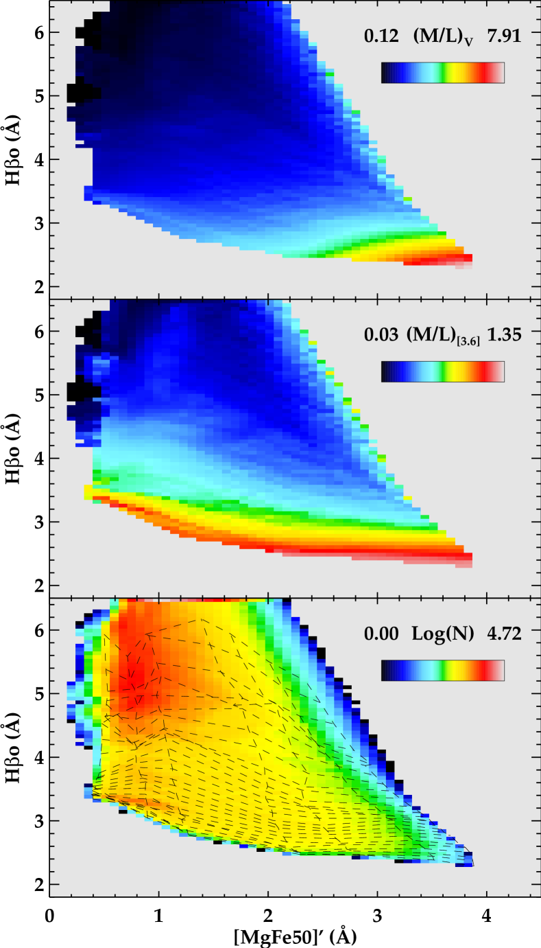
Figure 18: Stellar mass-to-light ratios ($\gamma_{\ast}$) predictions for the set of models produced by the combination of two single stellar populations. Top and middle panel show the median $M/L$ ratio in the $V-$ and $3.6\mu$m-band. The bottom panel shows a two-dimensional diagram with the number of models (in logarithmic scale) falling in a given bin in the H$\beta_{\rm o}$ vs [MgFe50]^′ space. For reference, dashed lines mark locations of equal age (along the vertical direction) and metallicity (along the abcissae) for a single stellar population.

We choose here to use as baseline SFHs different combinations of two stellar populations. While a library with different combinations might not accurately represent the SFH of any given galaxy, it will at least show the maximum range of $\gamma_{\ast}$ allowed for a given pair of H$\beta_{\rm o}$ and [MgFe50]^′ indices. We thus built a library of $\sim 5\times 10^{6}$ models by combining two single stellar populations in the age range from 0.1 to 17.28 Gyr (sampled logarithmically) and $[M/H]=$[-2.32,0.22] (sampled uniformly) for different mass fractions of the young component from 0 (i.e. an SSP) to 0.25. We set no restriction on the metallicities of the two components, and simply impose the age of the young one to be lower than the old one. Figure 18 shows the median $\gamma_{\ast}$, for the $V$- and $3.6\mu$m-bands, in the H$\beta_{\rm o}$ vs [MgFe50]^′ space. It also shows the number of models per bin. On average our library of models contains at least 1000 predictions per bin. Figure18 shows that $\gamma_{\ast}$ variations depend mostly on H$\beta_{\rm o}$ and that this dependency is stronger in the $3.6\mu$m-band than in the $V-$band.

We determine the best effective $\gamma_{\ast}$ via a Bayesian approach following Kauffmann et al. (2003) (see Appendix A in that paper for details). This method results into a probability distribution for a given set of plausible models. We take as effective $\gamma_{\ast}$ the weighted mean value of the distribution and the 68% confidence interval as its uncertainty. Measured values are listed in Tables 4 and  5.

Appendix C Dependence of kinematic substructure and environment in scaling relations

In this Appendix we show the main scaling relations in the $V$- and $3.6\mu$m-band, colour-coded according to kinematic substructure and environment. They are shown here, rather than in the main text, for completeness as they do not reveal any particular trend.

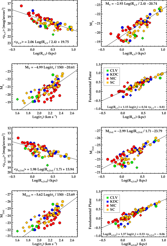
Figure 19: Scaling relations in the $V$- and $3.6\mu$m-band for the SAURON sample. Galaxies are colour-coded according to their level of kinematic substructure: (CLV) central low velocity, (KDC) kinematically decoupled core, (MC) multiple component, (SC) single component. Elliptical and lenticular galaxies are marked with circles, while Sa galaxies are denoted with diamonds. Best-fit relations as shown in §6 and §7.

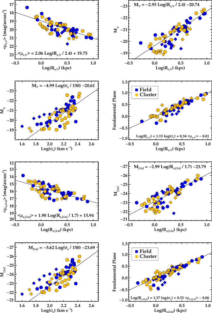
Figure 20: Scaling relations in the $V$- and $3.6\mu$m-band for the SAURON sample. Galaxies are colour-coded according to their environment as indicated. Elliptical and lenticular galaxies are marked with circles, while Sa galaxies are denoted with diamonds. Best-fit relations as shown in §6 and §7.

Appendix D Photometric & SAURON quantities

Here we present tables with the aperture photometry derived for the SAURON sample galaxies in both the $V$- and 3.6$\mu$m-bands, as described in the text (see § 4). We also give tables with the spectroscopic quantities derived from the SAURON data, as described in § 5 and Appendix B.

Table 2: Photometric quantities for the SAURON sample of E/S0 galaxies.

Galaxy	Env.	D	Ref.	Re,V	$\langle\mu_{\rm e,V}\rangle$	$M_{\rm V}$	AV	Re,[3.6]	$\langle\mu_{\rm e,[3.6]}\rangle$	$M_{\rm[3.6]}$	A[3.6]	$(V-[3.6])_{\rm e}$	nV	n[3.6]
		(Mpc)		(arcsec)	(mag arcsec-2)	(mag)	(mag)	(arcsec)	(mag arcsec-2)	(mag)	(mag)	(mag)
(1)	(2)	(3)	(4)	(5)	(6)	(7)	(8)	(9)	(10)	(11)	(12)	(13)	(14)	(15)
$0474$	F	$29.51$	$1$	$28.08\pm 1.65$	$20.72\pm 0.09$	$-20.87\pm 0.12$	$0.11$	$20.07\pm 0.37$	$20.72\pm 0.11$	$-23.94\pm 0.11$	$0.01$	$3.26\pm 0.05$	$4.0$	$4.0$
$0524$	F	$23.99$	$3$	$35.41\pm 1.02$	$19.90\pm 0.07$	$-21.75\pm 0.20$	$0.27$	$28.86\pm 0.26$	$19.90\pm 0.08$	$-25.04\pm 0.20$	$0.02$	$3.43\pm 0.03$	$2.8$	$2.8$
$0821$	F	$24.10$	$3$	$31.33\pm 1.49$	$20.09\pm 0.08$	$-21.30\pm 0.17$	$0.36$	$22.88\pm 0.46$	$20.09\pm 0.10$	$-24.31\pm 0.17$	$0.02$	$3.19\pm 0.04$	$4.0$	$4.0$
$1023$	F	$11.43$	$3$	$48.75\pm 1.46$	$19.65\pm 0.05$	$-21.08\pm 0.16$	$0.20$	$26.95\pm 0.19$	$19.65\pm 0.08$	$-24.08\pm 0.16$	$0.01$	$3.35\pm 0.02$	$4.0$	$3.0$
$2549$	F	$12.65$	$3$	$13.92\pm 0.43$	$18.84\pm 0.16$	$-19.38\pm 0.28$	$0.21$	$11.49\pm 0.08$	$18.84\pm 0.19$	$-22.56\pm 0.28$	$0.01$	$3.30\pm 0.02$	$2.9$	$2.9$
$2685$	F	$16.60$	$0$	$23.68\pm 1.16$	$20.02\pm 0.10$	$-19.95\pm 0.49$	$0.20$	$16.27\pm 0.41$	$20.02\pm 0.14$	$-22.94\pm 0.49$	$0.01$	$3.21\pm 0.04$	$4.0$	$3.5$
$2695$	F	$32.36$	$3$	$18.74\pm 1.26$	$20.05\pm 0.12$	$-20.86\pm 0.40$	$0.06$	$11.72\pm 0.13$	$20.05\pm 0.19$	$-23.96\pm 0.40$	$0.00$	$3.37\pm 0.04$	$4.0$	$3.1$
$2699$	F	$26.92$	$3$	$12.14\pm 0.95$	$19.59\pm 0.18$	$-19.97\pm 0.27$	$0.07$	$7.83\pm 0.08$	$19.59\pm 0.28$	$-22.99\pm 0.27$	$0.00$	$3.29\pm 0.05$	$4.0$	$2.9$
$2768$	F	$22.39$	$3$	$67.97\pm 3.11$	$20.94\pm 0.05$	$-21.97\pm 0.24$	$0.14$	$45.49\pm 0.28$	$20.94\pm 0.05$	$-25.03\pm 0.24$	$0.01$	$3.29\pm 0.04$	$4.0$	$3.5$
$2974$	F	$21.48$	$3$	$28.35\pm 1.61$	$19.87\pm 0.09$	$-21.05\pm 0.24$	$0.18$	$20.33\pm 0.11$	$19.87\pm 0.11$	$-24.27\pm 0.24$	$0.01$	$3.42\pm 0.04$	$4.0$	$3.4$
$3032$	F	$21.98$	$3$	$19.30\pm 1.07$	$20.41\pm 0.12$	$-19.73\pm 0.28$	$0.06$	$10.61\pm 0.09$	$20.41\pm 0.20$	$-22.49\pm 0.28$	$0.00$	$3.08\pm 0.04$	$3.6$	$3.6$
$3156$	F	$22.39$	$3$	$14.78\pm 0.44$	$20.02\pm 0.15$	$-19.58\pm 0.14$	$0.11$	$13.40\pm 0.14$	$20.02\pm 0.16$	$-22.39\pm 0.14$	$0.01$	$2.89\pm 0.03$	$2.4$	$2.4$
$3377$	C	$11.22$	$3$	$38.28\pm 1.99$	$20.02\pm 0.07$	$-20.14\pm 0.10$	$0.11$	$21.80\pm 0.22$	$20.02\pm 0.10$	$-22.92\pm 0.09$	$0.01$	$3.08\pm 0.04$	$4.0$	$4.0$
$3379$	C	$10.57$	$3$	$44.89\pm 1.47$	$19.47\pm 0.05$	$-20.90\pm 0.11$	$0.08$	$33.53\pm 0.40$	$19.47\pm 0.07$	$-24.04\pm 0.11$	$0.00$	$3.31\pm 0.03$	$4.0$	$4.0$
$3384$	C	$11.59$	$3$	$28.50\pm 0.91$	$19.15\pm 0.08$	$-20.44\pm 0.14$	$0.09$	$20.41\pm 0.09$	$19.15\pm 0.11$	$-23.57\pm 0.14$	$0.00$	$3.28\pm 0.02$	$4.0$	$4.0$
$3414$	F	$25.23$	$3$	$32.02\pm 1.45$	$20.31\pm 0.08$	$-21.22\pm 0.33$	$0.08$	$20.47\pm 0.23$	$20.31\pm 0.11$	$-24.29\pm 0.33$	$0.00$	$3.31\pm 0.03$	$4.0$	$4.0$
$3489$	C	$12.08$	$3$	$21.51\pm 0.81$	$18.82\pm 0.10$	$-20.25\pm 0.15$	$0.05$	$13.38\pm 0.14$	$18.82\pm 0.16$	$-23.14\pm 0.15$	$0.00$	$3.15\pm 0.02$	$4.0$	$3.0$
$3608$	F	$22.91$	$3$	$33.64\pm 1.52$	$20.34\pm 0.07$	$-21.09\pm 0.14$	$0.07$	$23.98\pm 0.15$	$20.34\pm 0.09$	$-24.14\pm 0.14$	$0.00$	$3.24\pm 0.04$	$4.0$	$4.0$
$4150$	C	$13.74$	$3$	$15.88\pm 0.52$	$19.62\pm 0.14$	$-19.07\pm 0.24$	$0.06$	$10.10\pm 0.09$	$19.62\pm 0.21$	$-22.04\pm 0.24$	$0.00$	$3.24\pm 0.02$	$2.6$	$2.6$
$4262$	C	$15.42$	$2$	$10.60\pm 0.43$	$18.53\pm 0.21$	$-19.54\pm 0.06$	$0.11$	$7.64\pm 0.07$	$18.53\pm 0.28$	$-22.71\pm 0.06$	$0.01$	$3.34\pm 0.02$	$4.0$	$4.0$
$4270$	C	$16.53$	$5$	$13.68\pm 0.47$	$19.74\pm 0.16$	$-19.02\pm 0.09$	$0.07$	$13.34\pm 0.14$	$19.74\pm 0.16$	$-22.21\pm 0.08$	$0.00$	$3.21\pm 0.03$	$2.2$	$2.2$
$4278$	C	$16.07$	$3$	$30.57\pm 1.07$	$19.48\pm 0.07$	$-20.97\pm 0.20$	$0.09$	$22.51\pm 0.39$	$19.48\pm 0.10$	$-24.14\pm 0.20$	$0.00$	$3.32\pm 0.02$	$4.0$	$4.0$
$4374$	C	$18.45$	$2$	$70.08\pm 2.95$	$20.17\pm 0.04$	$-22.39\pm 0.06$	$0.13$	$47.95\pm 0.60$	$20.17\pm 0.05$	$-25.46\pm 0.05$	$0.01$	$3.28\pm 0.03$	$4.0$	$4.0$
$4382$	C	$17.86$	$2$	$94.40\pm 3.17$	$20.58\pm 0.04$	$-22.55\pm 0.06$	$0.10$	$74.77\pm 0.70$	$20.58\pm 0.03$	$-25.60\pm 0.05$	$0.01$	$3.21\pm 0.04$	$4.0$	$4.0$
$4387$	C	$17.95$	$2$	$11.04\pm 0.22$	$19.33\pm 0.20$	$-19.15\pm 0.06$	$0.11$	$10.43\pm 0.08$	$19.33\pm 0.21$	$-22.28\pm 0.06$	$0.01$	$3.18\pm 0.02$	$2.1$	$2.1$
$4458$	C	$16.37$	$2$	$19.94\pm 0.96$	$20.46\pm 0.12$	$-19.11\pm 0.06$	$0.08$	$15.21\pm 0.14$	$20.46\pm 0.14$	$-21.99\pm 0.05$	$0.00$	$3.07\pm 0.04$	$3.1$	$2.9$
$4459$	C	$16.07$	$2$	$40.97\pm 1.48$	$20.09\pm 0.06$	$-21.00\pm 0.07$	$0.15$	$26.54\pm 0.36$	$20.09\pm 0.08$	$-24.12\pm 0.06$	$0.01$	$3.35\pm 0.03$	$4.0$	$4.0$
$4473$	C	$15.28$	$2$	$26.76\pm 0.89$	$19.29\pm 0.08$	$-20.76\pm 0.06$	$0.09$	$22.26\pm 0.31$	$19.29\pm 0.10$	$-23.97\pm 0.06$	$0.00$	$3.30\pm 0.02$	$4.0$	$4.4$
$4477$	C	$16.53$	$5$	$46.48\pm 2.22$	$20.48\pm 0.06$	$-20.94\pm 0.09$	$0.10$	$35.87\pm 0.69$	$20.48\pm 0.06$	$-24.10\pm 0.08$	$0.01$	$3.32\pm 0.04$	$4.0$	$4.0$
$4486$	C	$17.22$	$2$	$106.18\pm 4.23$	$20.60\pm 0.05$	$-22.70\pm 0.08$	$0.07$	$80.69\pm 0.71$	$20.60\pm 0.03$	$-25.98\pm 0.07$	$0.00$	$3.44\pm 0.04$	$4.0$	$4.0$
$4526$	C	$16.90$	$3$	$35.70\pm 1.29$	$19.44\pm 0.07$	$-21.46\pm 0.20$	$0.07$	$24.03\pm 0.22$	$19.44\pm 0.09$	$-24.75\pm 0.20$	$0.00$	$3.53\pm 0.03$	$3.3$	$3.2$
$4546$	C	$14.06$	$3$	$21.98\pm 0.94$	$19.03\pm 0.10$	$-20.41\pm 0.20$	$0.11$	$13.60\pm 0.10$	$19.03\pm 0.16$	$-23.48\pm 0.20$	$0.01$	$3.34\pm 0.03$	$4.0$	$3.4$
$4550$	C	$15.49$	$2$	$11.55\pm 0.27$	$19.00\pm 0.19$	$-19.26\pm 0.05$	$0.13$	$10.13\pm 0.06$	$19.00\pm 0.21$	$-22.30\pm 0.05$	$0.01$	$3.15\pm 0.02$	$1.8$	$1.8$
$4552$	C	$15.85$	$2$	$33.89\pm 1.09$	$19.43\pm 0.07$	$-21.21\pm 0.06$	$0.13$	$27.88\pm 0.21$	$19.43\pm 0.08$	$-24.53\pm 0.06$	$0.01$	$3.43\pm 0.02$	$4.0$	$4.0$
$4564$	C	$15.85$	$2$	$19.35\pm 1.11$	$19.41\pm 0.12$	$-20.02\pm 0.07$	$0.11$	$12.97\pm 0.21$	$19.41\pm 0.17$	$-23.13\pm 0.06$	$0.01$	$3.34\pm 0.04$	$4.0$	$3.4$
$4570$	C	$17.06$	$2$	$12.75\pm 0.56$	$18.48\pm 0.17$	$-20.20\pm 0.07$	$0.07$	$9.17\pm 0.08$	$18.48\pm 0.24$	$-23.33\pm 0.06$	$0.00$	$3.34\pm 0.03$	$4.0$	$2.4$
$4621$	C	$14.93$	$2$	$46.06\pm 2.99$	$19.96\pm 0.06$	$-21.22\pm 0.07$	$0.11$	$30.38\pm 0.39$	$19.96\pm 0.07$	$-24.32\pm 0.06$	$0.01$	$3.33\pm 0.04$	$4.0$	$4.0$
$4660$	C	$15.00$	$2$	$11.54\pm 0.41$	$18.44\pm 0.19$	$-19.75\pm 0.05$	$0.11$	$8.87\pm 0.11$	$18.44\pm 0.25$	$-22.89\pm 0.05$	$0.01$	$3.31\pm 0.02$	$4.0$	$4.0$
$5198$	F	$48.78$	$8$	$18.01\pm 0.69$	$20.09\pm 0.12$	$-21.62\pm 0.03$	$0.08$	$15.01\pm 0.14$	$20.09\pm 0.14$	$-24.80\pm 0.01$	$0.00$	$3.31\pm 0.03$	$2.5$	$2.5$
$5308$	F	$29.43$	$4$	$9.89\pm 0.25$	$18.72\pm 0.22$	$-20.60\pm 0.22$	$0.06$	$7.31\pm 0.04$	$18.72\pm 0.30$	$-23.73\pm 0.22$	$0.00$	$3.38\pm 0.02$	$4.0$	$1.7$
$5813$	F	$32.21$	$3$	$55.99\pm 2.72$	$20.94\pm 0.06$	$-22.33\pm 0.19$	$0.19$	$39.03\pm 0.62$	$20.94\pm 0.06$	$-25.42\pm 0.18$	$0.01$	$3.33\pm 0.05$	$4.0$	$4.0$
$5831$	F	$27.16$	$3$	$29.19\pm 1.70$	$20.45\pm 0.08$	$-21.04\pm 0.17$	$0.19$	$21.82\pm 0.27$	$20.45\pm 0.10$	$-24.11\pm 0.17$	$0.01$	$3.23\pm 0.04$	$4.0$	$4.0$
$5838$	F	$23.99$	$0$	$20.61\pm 0.87$	$19.29\pm 0.11$	$-21.18\pm 0.49$	$0.17$	$15.25\pm 0.12$	$19.29\pm 0.14$	$-24.43\pm 0.49$	$0.01$	$3.41\pm 0.03$	$4.0$	$3.8$
$5845$	F	$25.94$	$3$	$4.29\pm 0.26$	$17.37\pm 0.51$	$-19.86\pm 0.21$	$0.17$	$3.59\pm 0.08$	$17.37\pm 0.61$	$-22.98\pm 0.21$	$0.01$	$3.29\pm 0.05$	$4.0$	$4.0$
$5846$	F	$24.89$	$3$	$76.79\pm 3.32$	$21.03\pm 0.05$	$-22.37\pm 0.21$	$0.18$	$64.39\pm 0.61$	$21.03\pm 0.04$	$-25.62\pm 0.20$	$0.01$	$3.35\pm 0.05$	$4.0$	$4.0$
$5982$	F	$40.36$	$1$	$24.89\pm 1.19$	$20.03\pm 0.09$	$-21.97\pm 0.09$	$0.06$	$19.65\pm 0.19$	$20.03\pm 0.11$	$-25.23\pm 0.09$	$0.00$	$3.38\pm 0.03$	$4.0$	$4.0$
$7332$	F	$23.01$	$3$	$9.21\pm 0.15$	$18.09\pm 0.24$	$-20.54\pm 0.20$	$0.12$	$8.14\pm 0.04$	$18.09\pm 0.27$	$-23.64\pm 0.20$	$0.01$	$3.20\pm 0.01$	$2.0$	$2.0$
$7457$	F	$13.24$	$3$	$33.25\pm 1.28$	$20.59\pm 0.08$	$-19.63\pm 0.21$	$0.17$	$27.37\pm 0.19$	$20.59\pm 0.08$	$-22.55\pm 0.21$	$0.01$	$3.08\pm 0.04$	$2.5$	$2.5$

NOTES: (1) NGC galaxy number. (2) Environment: Field (F) or Cluster (C). (3) Distance (Mpc). (4) Original reference for the distance estimate (0: redshift distance from NED; 1: Cantiello et al. 2007; 2: Mei et al. 2007; 3: Tonry et al. 2001; 4: Reindl et al. 2005; 5: Mei et al. 2007, but see (iii) in §3.3; 6: Terry et al. 2002; 7: Tully et al. 2008; 8: Willick et al. 1997). See §3.3 for uncertainties in the measurements, (5-12) Photometric quantities: effective radii ($R_{\rm e}$), mean effective surface brightness ($\langle\mu_{\rm e}\rangle$), absolute magnitude (M) and Galactic extinction in the $V$- and $3.6\mu$m bands. (13) Effective $(V-[3.6])$ colour. (14-15) Sérsic indices used in our growth curve analysis (see §4).

Table 3: Photometric quantities for the SAURON sample of Sa galaxies.

Galaxy	Env.	D	Ref.	Re,V	$\langle\mu_{\rm e,V}\rangle$	$M_{\rm V}$	AV	Re,[3.6]	$\langle\mu_{\rm e,[3.6]}\rangle$	$M_{\rm[3.6]}$	A[3.6]	$(V-[3.6])_{\rm e}$	nV	n[3.6]
		(Mpc)		(arcsec)	(mag arcsec-2)	(mag)	(mag)	(arcsec)	(mag arcsec-2)	(mag)	(mag)	(mag)
(1)	(2)	(3)	(4)	(5)	(6)	(7)	(8)	(9)	(10)	(11)	(12)	(13)	(14)	(15)
$1056$	F	$32.21$	$7$	$17.48\pm 1.24$	$20.17\pm 0.13$	$-20.57\pm 0.40$	$0.48$	$7.14\pm 0.32$	$20.17\pm 0.31$	$-23.84\pm 0.40$	$0.03$	$3.70\pm 0.06$	$4.0$	$4.0$
$2273$	F	$31.62$	$6$	$27.64\pm 1.22$	$20.53\pm 0.09$	$-21.17\pm 0.39$	$0.23$	$17.78\pm 0.65$	$20.53\pm 0.12$	$-24.56\pm 0.39$	$0.01$	$3.64\pm 0.04$	$2.9$	$6.6$
$2844$	F	$25.12$	$0$	$16.91\pm 1.23$	$20.72\pm 0.14$	$-19.42\pm 0.49$	$0.06$	$7.39\pm 0.11$	$20.72\pm 0.29$	$-22.39\pm 0.49$	$0.00$	$3.41\pm 0.05$	$4.0$	$2.9$
$3623$	C	$11.97$	$7$	$48.21\pm 0.95$	$19.73\pm 0.05$	$-21.07\pm 0.35$	$0.08$	$31.99\pm 0.32$	$19.73\pm 0.07$	$-24.14\pm 0.35$	$0.00$	$3.45\pm 0.03$	$2.1$	$1.5$
$4220$	F	$18.79$	$7$	$20.30\pm 0.50$	$20.08\pm 0.11$	$-19.82\pm 0.36$	$0.06$	$13.50\pm 0.08$	$20.08\pm 0.16$	$-23.10\pm 0.36$	$0.00$	$3.62\pm 0.03$	$1.6$	$2.1$
$4235$	C	$16.53$	$5$	$16.44\pm 0.49$	$19.96\pm 0.13$	$-19.21\pm 0.09$	$0.06$	$12.30\pm 0.24$	$19.96\pm 0.18$	$-22.74\pm 0.08$	$0.00$	$3.71\pm 0.03$	$1.9$	$1.9$
$4245$	C	$13.18$	$0$	$35.95\pm 1.63$	$20.77\pm 0.07$	$-19.60\pm 0.49$	$0.07$	$22.14\pm 0.23$	$20.77\pm 0.10$	$-22.50\pm 0.49$	$0.00$	$3.24\pm 0.04$	$3.5$	$3.5$
$4274$	C	$19.41$	$7$	$45.43\pm 1.26$	$20.56\pm 0.06$	$-21.16\pm 0.36$	$0.07$	$33.70\pm 0.16$	$20.56\pm 0.06$	$-24.45\pm 0.36$	$0.00$	$3.53\pm 0.03$	$2.3$	$1.6$
$4293$	C	$16.53$	$5$	$52.20\pm 1.63$	$21.09\pm 0.06$	$-20.59\pm 0.09$	$0.13$	$31.00\pm 0.48$	$21.09\pm 0.07$	$-23.51\pm 0.08$	$0.01$	$3.36\pm 0.05$	$1.8$	$2.4$
$4314$	C	$17.38$	$0$	$46.90\pm 2.24$	$20.74\pm 0.06$	$-20.81\pm 0.49$	$0.08$	$32.80\pm 0.59$	$20.74\pm 0.07$	$-23.94\pm 0.49$	$0.00$	$3.31\pm 0.03$	$4.0$	$3.0$
$4369$	F	$20.89$	$0$	$24.73\pm 1.27$	$20.38\pm 0.09$	$-20.18\pm 0.49$	$0.08$	$14.67\pm 0.15$	$20.38\pm 0.15$	$-23.01\pm 0.49$	$0.00$	$3.13\pm 0.04$	$4.0$	$2.7$
$4383$	C	$16.53$	$5$	$14.83\pm 0.79$	$19.77\pm 0.15$	$-19.18\pm 0.09$	$0.08$	$9.98\pm 0.19$	$19.77\pm 0.22$	$-22.30\pm 0.08$	$0.00$	$3.32\pm 0.03$	$4.0$	$4.0$
$4405$	C	$16.53$	$5$	$18.29\pm 0.48$	$20.51\pm 0.12$	$-18.89\pm 0.09$	$0.08$	$12.95\pm 0.17$	$20.51\pm 0.17$	$-21.83\pm 0.08$	$0.00$	$3.25\pm 0.04$	$1.2$	$1.2$
$4425$	C	$16.53$	$5$	$15.91\pm 0.65$	$20.03\pm 0.14$	$-19.07\pm 0.09$	$0.09$	$12.36\pm 0.09$	$20.03\pm 0.18$	$-22.00\pm 0.08$	$0.00$	$3.14\pm 0.04$	$2.0$	$2.0$
$4596$	C	$16.53$	$5$	$59.91\pm 3.05$	$20.93\pm 0.06$	$-21.05\pm 0.09$	$0.07$	$38.24\pm 0.45$	$20.93\pm 0.06$	$-24.02\pm 0.08$	$0.00$	$3.25\pm 0.05$	$4.0$	$4.0$
$4698$	C	$16.53$	$5$	$50.64\pm 2.40$	$20.76\pm 0.06$	$-20.85\pm 0.09$	$0.08$	$33.74\pm 0.22$	$20.76\pm 0.06$	$-23.80\pm 0.08$	$0.00$	$3.22\pm 0.04$	$4.0$	$3.0$
$4772$	C	$16.53$	$5$	$42.71\pm 2.34$	$21.08\pm 0.07$	$-20.16\pm 0.09$	$0.09$	$25.26\pm 0.31$	$21.08\pm 0.09$	$-23.01\pm 0.08$	$0.00$	$3.14\pm 0.05$	$4.0$	$4.0$
$5448$	F	$34.83$	$6$	$24.97\pm 0.87$	$20.88\pm 0.10$	$-20.81\pm 0.18$	$0.05$	$17.09\pm 0.26$	$20.88\pm 0.13$	$-24.00\pm 0.18$	$0.00$	$3.48\pm 0.04$	$1.8$	$3.0$
$5475$	F	$30.20$	$0$	$9.42\pm 0.23$	$19.54\pm 0.23$	$-19.73\pm 0.49$	$0.04$	$7.78\pm 0.07$	$19.54\pm 0.28$	$-22.95\pm 0.49$	$0.00$	$3.36\pm 0.02$	$1.3$	$2.4$
$5636$	F	$28.84$	$0$	$22.89\pm 0.89$	$21.72\pm 0.11$	$-19.38\pm 0.49$	$0.11$	$16.65\pm 0.24$	$21.72\pm 0.13$	$-21.81\pm 0.49$	$0.01$	$2.85\pm 0.07$	$1.0$	$1.0$
$5689$	F	$36.31$	$0$	$12.63\pm 0.35$	$19.29\pm 0.17$	$-21.02\pm 0.49$	$0.12$	$7.91\pm 0.04$	$19.29\pm 0.27$	$-24.24\pm 0.49$	$0.01$	$3.56\pm 0.03$	$2.1$	$2.1$
$5953$	F	$33.11$	$0$	$12.84\pm 0.72$	$19.53\pm 0.17$	$-20.61\pm 0.49$	$0.16$	$6.88\pm 0.14$	$19.53\pm 0.32$	$-24.03\pm 0.49$	$0.01$	$3.71\pm 0.04$	$4.0$	$4.0$
$6501$	F	$47.86$	$0$	$20.27\pm 1.40$	$20.37\pm 0.12$	$-21.56\pm 0.49$	$0.29$	$14.02\pm 0.33$	$20.37\pm 0.16$	$-24.73\pm 0.49$	$0.02$	$3.35\pm 0.05$	$4.0$	$5.9$
$7742$	F	$22.91$	$0$	$13.93\pm 0.36$	$19.17\pm 0.16$	$-20.35\pm 0.49$	$0.18$	$12.05\pm 0.07$	$19.17\pm 0.18$	$-23.41\pm 0.49$	$0.01$	$3.18\pm 0.02$	$2.1$	$2.1$

NOTES: (1) NGC galaxy number. (2) Environment: Field (F) or Cluster (C). (3) Distance (Mpc). (4) Original reference for the distance estimate (0: redshift distance from NED; 1: Cantiello et al. 2007; 2: Mei et al. 2007; 3: Tonry et al. 2001; 4: Reindl et al. 2005; 5: Mei et al. 2007, but see (iii) in §3.3; 6: Terry et al. 2002; 7: Tully et al. 2008; 8: Willick et al. 1997). See §3.3 for uncertainties in the measurements, (5-12) Photometric quantities: effective radii ($R_{\rm e}$), mean effective surface brightness ($\langle\mu_{\rm e}\rangle$), absolute magnitude (M) and Galactic extinction in the $V$- and $3.6\mu$m bands. (13) Effective $(V-[3.6])$ colour. (14-15) Sérsic indices used in our growth curve analysis (see §4).

Table 4: Spectroscopic quantities for the SAURON sample of E/S0 galaxies.

Galaxy	SR/FR	Kinem.	$\sigma_{\rm e}$	H$\beta$	H$\beta_{o}$	Fe5015	Mg$b$	$\gamma_{\ast,V}$	$\gamma_{\ast,[3.6]}$
			(km/s)	(Å)	(Å)	(Å)	(Å)	(${\rm M_{\odot}/L_{\odot}}$)V	(${\rm M_{\odot}/L_{\odot}}$)[3.6]
(1)	(2)	(3)	(4)	(5)	(6)	(7)	(8)	(9)	(10)
$0474$	FR	MC	$142$	$1.85$	$2.93$	$3.84$	$2.96$	$3.52_{-0.59}^{+0.67}$	$0.78_{-0.13}^{+0.14}$
$0524$	FR	SC	$225$	$1.52$	$2.58$	$4.26$	$3.63$	$5.36_{-0.60}^{+0.58}$	$1.05_{-0.10}^{+0.10}$
$0821$	FR	SC	$182$	$1.65$	$2.65$	$3.69$	$3.22$	$4.54_{-0.60}^{+0.63}$	$1.02_{-0.12}^{+0.12}$
$1023$	FR	SC	$165$	$1.57$	$2.55$	$3.85$	$3.55$	$5.17_{-0.57}^{+0.56}$	$1.09_{-0.11}^{+0.11}$
$2549$	FR	MC	$140$	$2.01$	$3.26$	$4.14$	$3.10$	$2.68_{-0.65}^{+0.90}$	$0.53_{-0.13}^{+0.17}$
$2685$	FR	SC	$100$	$2.05$	$3.09$	$3.33$	$2.59$	$2.88_{-0.69}^{+0.74}$	$0.72_{-0.18}^{+0.18}$
$2695$	FR	MC	$184$	$1.36$	$2.19$	$3.39$	$3.44$	$5.01_{-0.28}^{+0.28}$	$1.21_{-0.05}^{+0.03}$
$2699$	FR	MC	$123$	$1.78$	$2.83$	$3.81$	$3.11$	$3.91_{-0.57}^{+0.65}$	$0.87_{-0.13}^{+0.13}$
$2768$	FR	SC	$200$	$1.67$	$2.67$	$3.47$	$3.12$	$4.28_{-0.62}^{+0.65}$	$1.02_{-0.13}^{+0.12}$
$2974$	FR	SC	$227$	$1.73$	$2.77$	$4.01$	$3.50$	$4.33_{-0.56}^{+0.60}$	$0.89_{-0.12}^{+0.11}$
$3032$	FR	CLV	$90$	$3.85$	$5.30$	$3.19$	$1.74$	$1.31_{-0.58}^{+0.85}$	$0.30_{-0.14}^{+0.20}$
$3156$	FR	SC	$66$	$2.93$	$4.16$	$2.90$	$1.55$	$1.45_{-0.47}^{+0.70}$	$0.41_{-0.14}^{+0.22}$
$3377$	FR	SC	$126$	$1.95$	$3.10$	$3.48$	$2.74$	$2.88_{-0.68}^{+0.72}$	$0.69_{-0.17}^{+0.17}$
$3379$	FR	SC	$190$	$1.54$	$2.60$	$3.74$	$3.53$	$4.90_{-0.59}^{+0.58}$	$1.06_{-0.11}^{+0.11}$
$3384$	FR	MC	$141$	$1.87$	$2.98$	$4.05$	$3.17$	$3.40_{-0.64}^{+0.66}$	$0.71_{-0.14}^{+0.13}$
$3414$	SR	KDC	$191$	$1.58$	$2.47$	$3.49$	$3.17$	$4.74_{-0.43}^{+0.45}$	$1.14_{-0.09}^{+0.08}$
$3489$	FR	MC	$99$	$2.53$	$3.65$	$3.47$	$2.21$	$1.94_{-0.54}^{+0.78}$	$0.46_{-0.15}^{+0.20}$
$3608$	SR	KDC	$167$	$1.71$	$2.78$	$3.73$	$3.24$	$4.10_{-0.59}^{+0.64}$	$0.91_{-0.13}^{+0.12}$
$4150$	FR	CLV	$77$	$2.69$	$3.57$	$3.27$	$2.00$	$2.02_{-0.60}^{+0.79}$	$0.52_{-0.17}^{+0.22}$
$4262$	FR	MC	$164$	$1.52$	$2.45$	$3.45$	$3.33$	$4.84_{-0.43}^{+0.42}$	$1.15_{-0.09}^{+0.07}$
$4270$	FR	MC	$125$	$1.77$	$2.72$	$3.64$	$2.77$	$4.10_{-0.63}^{+0.68}$	$0.98_{-0.13}^{+0.13}$
$4278$	FR	MC	$217$	$1.65$	$2.73$	$3.62$	$3.63$	$4.37_{-0.57}^{+0.63}$	$0.95_{-0.12}^{+0.12}$
$4374$	SR	SC	$261$	$1.49$	$2.48$	$3.61$	$3.47$	$5.06_{-0.48}^{+0.48}$	$1.14_{-0.10}^{+0.08}$
$4382$	FR	CLV	$178$	$1.99$	$3.09$	$3.63$	$2.80$	$2.93_{-0.66}^{+0.71}$	$0.67_{-0.16}^{+0.16}$
$4387$	FR	MC	$98$	$1.60$	$2.51$	$3.58$	$3.18$	$4.78_{-0.49}^{+0.49}$	$1.12_{-0.11}^{+0.09}$
$4458$	SR	KDC	$83$	$1.64$	$2.46$	$3.17$	$2.88$	$4.18_{-0.37}^{+0.36}$	$1.15_{-0.10}^{+0.08}$
$4459$	FR	MC	$155$	$1.92$	$3.07$	$3.62$	$2.91$	$2.99_{-0.68}^{+0.70}$	$0.68_{-0.16}^{+0.16}$
$4473$	FR	MC	$186$	$1.56$	$2.54$	$3.82$	$3.45$	$5.11_{-0.57}^{+0.54}$	$1.10_{-0.11}^{+0.10}$
$4477$	FR	SC	$147$	$1.60$	$2.61$	$3.70$	$3.29$	$4.71_{-0.59}^{+0.59}$	$1.05_{-0.12}^{+0.12}$
$4486$	SR	SC	$268$	$1.25$	$2.21$	$3.52$	$3.87$	$5.56_{-0.30}^{+0.30}$	$1.21_{-0.05}^{+0.03}$
$4526$	FR	MC	$214$	$1.68$	$2.70$	$3.89$	$3.58$	$4.61_{-0.56}^{+0.61}$	$0.96_{-0.11}^{+0.11}$
$4546$	FR	MC	$189$	$1.60$	$2.49$	$3.64$	$3.39$	$5.02_{-0.49}^{+0.48}$	$1.13_{-0.10}^{+0.09}$
$4550$	SR	SC	$103$	$2.01$	$3.06$	$3.46$	$2.55$	$2.97_{-0.69}^{+0.73}$	$0.73_{-0.17}^{+0.17}$
$4552$	SR	KDC	$233$	$1.55$	$2.64$	$4.06$	$3.79$	$5.03_{-0.58}^{+0.60}$	$1.00_{-0.10}^{+0.10}$
$4564$	FR	SC	$150$	$1.62$	$2.65$	$3.84$	$3.47$	$4.75_{-0.59}^{+0.62}$	$1.01_{-0.11}^{+0.11}$
$4570$	FR	MC	$167$	$1.51$	$2.45$	$3.75$	$3.43$	$5.24_{-0.47}^{+0.45}$	$1.15_{-0.09}^{+0.08}$
$4621$	FR	KDC	$200$	$1.50$	$2.41$	$3.70$	$3.56$	$5.34_{-0.44}^{+0.41}$	$1.17_{-0.09}^{+0.06}$
$4660$	FR	MC	$181$	$1.55$	$2.59$	$3.72$	$3.48$	$4.89_{-0.57}^{+0.59}$	$1.07_{-0.11}^{+0.11}$
$5198$	SR	KDC	$173$	$1.60$	$2.59$	$3.75$	$3.43$	$4.89_{-0.57}^{+0.58}$	$1.07_{-0.11}^{+0.11}$
$5308$	FR	MC	$201$	$1.52$	$2.49$	$3.83$	$3.60$	$5.36_{-0.53}^{+0.50}$	$1.13_{-0.10}^{+0.09}$
$5813$	SR	KDC	$210$	$1.54$	$2.61$	$3.75$	$3.47$	$4.84_{-0.59}^{+0.59}$	$1.05_{-0.11}^{+0.12}$
$5831$	SR	KDC	$148$	$1.87$	$2.96$	$3.86$	$2.87$	$3.40_{-0.62}^{+0.68}$	$0.76_{-0.14}^{+0.15}$
$5838$	FR	MC	$232$	$1.66$	$2.67$	$3.94$	$3.58$	$4.76_{-0.57}^{+0.62}$	$0.99_{-0.11}^{+0.11}$
$5845$	FR	MC	$237$	$1.57$	$2.65$	$4.19$	$3.76$	$5.03_{-0.57}^{+0.61}$	$0.99_{-0.10}^{+0.10}$
$5846$	SR	SC	$213$	$1.35$	$2.36$	$3.74$	$3.60$	$5.48_{-0.42}^{+0.37}$	$1.18_{-0.09}^{+0.05}$
$5982$	SR	KDC	$223$	$1.63$	$2.66$	$4.05$	$3.38$	$4.79_{-0.57}^{+0.62}$	$1.00_{-0.11}^{+0.11}$
$7332$	FR	KDC	$125$	$2.10$	$3.27$	$3.87$	$2.75$	$2.53_{-0.61}^{+0.76}$	$0.55_{-0.14}^{+0.17}$
$7457$	FR	CLV	$75$	$2.26$	$3.40$	$3.60$	$2.40$	$2.27_{-0.59}^{+0.75}$	$0.53_{-0.15}^{+0.19}$

NOTES: (1) NGC galaxy number. (2) Slow/Fast Rotator class. (3) Kinematic substructure as defined in Paper XII. (4) Stellar velocity dispersion within $R_{\rm e,V}$. (5-8) Line-strength indices within $R_{\rm e,V}$ measured in the LIS-14Å system. (9-10) Stellar mass-to-light ratios ($\gamma_{\ast}$) in the $V$- and $3.6\mu$m bands.

Table 5: Spectroscopic quantities for the SAURON sample of Sa galaxies.

Galaxy	SR/FR	Kinem.	$\sigma_{\rm e}$	H$\beta$	H$\beta_{o}$	Fe5015	Mg$b$	$\gamma_{\ast,V}$	$\gamma_{\ast,[3.6]}$
			(km/s)	(Å)	(Å)	(Å)	(Å)	(${\rm M_{\odot}/L_{\odot}}$)V	(${\rm M_{\odot}/L_{\odot}}$)[3.6]
(1)	(2)	(3)	(4)	(5)	(6)	(7)	(8)	(9)	(10)
$1056$	FR	SC	$83$	$2.85$	$3.94$	$1.76$	$1.24$	$1.47_{-0.41}^{+0.46}$	$0.60_{-0.14}^{+0.18}$
$2273$	FR	MC	$124$	$2.72$	$3.98$	$3.13$	$2.27$	$1.63_{-0.50}^{+0.75}$	$0.40_{-0.14}^{+0.20}$
$2844$	FR	SC	$93$	$2.45$	$3.49$	$2.56$	$1.70$	$1.96_{-0.61}^{+0.75}$	$0.64_{-0.21}^{+0.23}$
$3623$	FR	MC	$141$	$1.69$	$2.70$	$3.70$	$3.27$	$4.39_{-0.59}^{+0.65}$	$0.98_{-0.12}^{+0.12}$
$4220$	FR	SC	$92$	$2.61$	$3.68$	$3.89$	$2.40$	$2.04_{-0.59}^{+0.83}$	$0.43_{-0.13}^{+0.17}$
$4235$	FR	MC	$165$	$1.84$	$2.69$	$3.67$	$2.97$	$4.29_{-0.61}^{+0.66}$	$1.00_{-0.13}^{+0.13}$
$4245$	FR	MC	$97$	$1.94$	$2.95$	$3.43$	$2.76$	$3.31_{-0.63}^{+0.73}$	$0.81_{-0.14}^{+0.16}$
$4274$	FR	MC	$153$	$1.88$	$2.89$	$3.51$	$2.85$	$3.53_{-0.62}^{+0.71}$	$0.85_{-0.14}^{+0.15}$
$4293$	FR	SC	$107$	$2.44$	$3.53$	$3.71$	$2.30$	$2.12_{-0.56}^{+0.79}$	$0.48_{-0.14}^{+0.20}$
$4314$	FR	SC	$118$	$2.13$	$3.13$	$3.37$	$2.60$	$2.79_{-0.70}^{+0.74}$	$0.69_{-0.18}^{+0.18}$
$4369$	FR	SC	$59$	$3.39$	$4.72$	$1.99$	$1.30$	$1.07_{-0.41}^{+0.60}$	$0.36_{-0.15}^{+0.21}$
$4383$	FR	SC	$51$	$3.05$	$4.05$	$0.40$	$0.89$	$1.15_{-0.25}^{+0.40}$	$0.63_{-0.10}^{+0.25}$
$4405$	FR	SC	$54$	$3.13$	$4.36$	$2.34$	$1.53$	$1.21_{-0.37}^{+0.64}$	$0.37_{-0.12}^{+0.24}$
$4425$	FR	CLV	$78$	$1.89$	$2.90$	$3.62$	$2.78$	$3.52_{-0.62}^{+0.70}$	$0.83_{-0.14}^{+0.15}$
$4596$	FR	MC	$156$	$1.66$	$2.62$	$3.51$	$3.21$	$4.49_{-0.58}^{+0.61}$	$1.05_{-0.12}^{+0.12}$
$4698$	FR	KDC	$141$	$1.67$	$2.59$	$3.30$	$2.90$	$4.20_{-0.55}^{+0.53}$	$1.08_{-0.13}^{+0.11}$
$4772$	FR	SC	$131$	$1.54$	$2.50$	$3.07$	$3.19$	$4.27_{-0.43}^{+0.42}$	$1.13_{-0.11}^{+0.09}$
$5448$	FR	MC	$128$	$2.19$	$3.27$	$3.23$	$2.65$	$2.50_{-0.68}^{+0.79}$	$0.62_{-0.18}^{+0.20}$
$5475$	FR	SC	$101$	$2.17$	$3.35$	$4.07$	$2.85$	$2.49_{-0.62}^{+0.88}$	$0.51_{-0.13}^{+0.17}$
$5636$	FR	CLV	$40$	$2.49$	$3.64$	$2.53$	$1.75$	$1.81_{-0.59}^{+0.73}$	$0.58_{-0.20}^{+0.24}$
$5689$	FR	MC	$166$	$1.98$	$3.12$	$4.02$	$2.93$	$2.91_{-0.64}^{+0.74}$	$0.61_{-0.14}^{+0.15}$
$5953$	FR	KDC	$100$	$2.86$	$3.97$	$1.69$	$1.29$	$1.44_{-0.39}^{+0.46}$	$0.60_{-0.14}^{+0.18}$
$6501$	FR	SC	$190$	$1.65$	$2.65$	$4.06$	$3.58$	$4.91_{-0.57}^{+0.61}$	$1.00_{-0.11}^{+0.11}$
$7742$	FR	KDC	$71$	$2.81$	$4.07$	$2.87$	$2.04$	$1.53_{-0.49}^{+0.72}$	$0.40_{-0.14}^{+0.21}$

NOTES: (1) NGC galaxy number. (2) Slow/Fast Rotator class. (3) Kinematic substructure as defined in Paper XII. (4) Stellar velocity dispersion within $R_{\rm e,V}$. (5-8) Line-strength indices within $R_{\rm e,V}$ measured in the LIS-14Å system. (9-10) Stellar mass-to-light ratios ($\gamma_{\ast}$) in the $V$- and $3.6\mu$m bands.

References

- Allanson et al. (2009) Allanson S. P., Hudson M. J., Smith R. J., Lucey J. R., 2009, ApJ, 702, 1275
- Andreon (2006) Andreon S., 2006, MNRAS, 369, 969
- Arnouts et al. (2007) Arnouts S., Walcher C. J., Le Fèvre O., Zamorani G., Ilbert O., Le Brun V., Pozzetti L., Bardelli S., et al. 2007, A&A, 476, 137
- Bacon et al. (2001) Bacon R., Copin Y., Monnet G., Miller B. W., Allington-Smith J. R., Bureau M., Carollo C. M., Davies R. L., et al., 2001, MNRAS, 326, 23 [Paper I]
- Balcells et al. (2007) Balcells M., Graham A. W., Peletier R. F., 2007, ApJ, 665, 1104
- Baldry et al. (2004) Baldry I. K., Glazebrook K., Brinkmann J., Ž. Ivezić Lupton R. H., Nichol R. C., Szalay A. S., 2004, ApJ, 600, 681
- Bell & de Jong (2001) Bell E. F., de Jong R. S., 2001, ApJ, 550, 212
- Bell et al. (2004) Bell E. F., Wolf C., Meisenheimer K., Rix H.-W., Borch A., Dye S., Kleinheinrich M., Wisotzki L., et al., 2004, ApJ, 608, 752
- Bender et al. (1992) Bender R., Burstein D., Faber S. M., 1992, ApJ, 399, 462
- Bernardi et al. (2003) Bernardi M., Sheth R. K., Annis J., Burles S., Eisenstein D. J., Finkbeiner D. P., Hogg D. W., et al. 2003, AJ, 125, 1817 [B03]
- Bernardi et al. (2003) Bernardi M., Sheth R. K., Annis J., Burles S., Eisenstein D. J., Finkbeiner D. P., Hogg D. W., Lupton R. H., et al. 2003, AJ, 125, 1866
- Bernardi et al. (2005) Bernardi M., Sheth R. K., Nichol R. C., Schneider D. P., Brinkmann J., 2005, AJ, 129, 61
- Bertin & Arnouts (1996) Bertin E., Arnouts S., 1996, A&AS, 117, 393
- Bolton et al. (2008) Bolton A. S., Treu T., Koopmans L. V. E., Gavazzi R., Moustakas L. A., Burles S., Schlegel D. J., Wayth R., 2008, ApJ, 684, 248
- Bower et al. (1992) Bower R. G., Lucey J. R., Ellis R. S., 1992, MNRAS, 254, 601
- Burstein et al. (1987) Burstein D., Davies R. L., Dressler A., Faber S. M., Stone R. P. S., Lynden-Bell D., Terlevich R. J., Wegner G., 1987, ApJS, 64, 601
- Busarello et al. (1997) Busarello G., Capaccioli M., Capozziello S., Longo G., Puddu E., 1997, A&A, 320, 415
- Byun et al. (1996) Byun Y.-I., Grillmair C. J., Faber S. M., Ajhar E. A., Dressler A., Kormendy J., Lauer T. R., Richstone D., et al., 1996, AJ, 111, 1889
- Cantiello et al. (2007) Cantiello M., Blakeslee J., Raimondo G., Brocato E., Capaccioli M., 2007, ApJ, 668, 130
- Caon et al. (1993) Caon N., Capaccioli M., D’Onofrio M., 1993, MNRAS, 265, 1013
- Cappellari (2002) Cappellari M., 2002, MNRAS, 333, 400
- Cappellari et al. (2006) Cappellari M., Bacon R., Bureau M., Damen M. C., Davies R. L., de Zeeuw P. T., Emsellem E., Falcón-Barroso J., et al., 2006, MNRAS, 366, 1126 [Paper IV]
- Cappellari & Emsellem (2004) Cappellari M., Emsellem E., 2004, PASP, 116, 138
- Cappellari et al. (2007) Cappellari M., Emsellem E., Bacon R., Bureau M., Davies R. L., de Zeeuw P. T., Falcón-Barroso J., Krajnović D., et al., 2007, MNRAS, 379, 418 [Paper X]
- Cappellari et al. (2011) Cappellari M., Emsellem E., Krajnović D., McDermid R.M., Scott N., Verdoes Kleijn G.A., Young L.M., Alatalo K. et al. 2011, MNRAS, 413, 813
- Carlberg (1984) Carlberg R. G., 1984, ApJ, 286, 403
- Carollo et al. (1997) Carollo C. M., Franx M., Illingworth G. D., Forbes D. A., 1997, ApJ, 481, 710
- Cervantes & Vazdekis (2009) Cervantes J. L., Vazdekis A., 2009, MNRAS, 392, 691
- Ciotti & Bertin (1999) Ciotti L., Bertin G., 1999, A&A, 352, 447
- Ciotti et al. (1996) Ciotti L., Lanzoni B., Renzini A., 1996, MNRAS, 282, 1
- Combes et al. (2007) Combes F., Young L. M., Bureau M., 2007, MNRAS, 377, 1795
- Conselice et al. (2005) Conselice C. J., Bundy K., Ellis R. S., Brichmann J., Vogt N. P., Phillips A. C., 2005, ApJ, 628, 160
- Courteau et al. (2007) Courteau S., Dutton A. A., van den Bosch F. C., MacArthur L. A., Dekel A., McIntosh D. H., Dale D. A., 2007, ApJ, 671, 203
- Crook et al. (2007) Crook A. C., Huchra J. P., Martimbeau N., Masters K. L., Jarrett T., Macri L. M., 2007, ApJ, 655, 790
- de Jong (2008) de Jong R. S., 2008, ArXiv e-prints, 807
- De Lucia et al. (2004) De Lucia G., Poggianti B. M., Aragón-Salamanca A., Clowe D., Halliday C., Jablonka P., Milvang-Jensen B., Pelló R., Poirier S., Rudnick G., Saglia R., Simard L., White S. D. M., 2004, ApJ, 610, L77
- de Vaucouleurs (1961) de Vaucouleurs G., 1961, ApJS, 5, 233
- de Vaucouleurs et al. (1991) de Vaucouleurs G., de Vaucouleurs A., Corwin J. H. G., Buta R. J., Paturel G., Fouque P., 1991, Third Reference Catalogue of Bright Galaxies. Volume 1-3, XII, 2069 pp. 7 figs.. Springer-Verlag Berlin Heidelberg New York
- de Zeeuw et al. (2002) de Zeeuw P. T., Bureau M., Emsellem E., Bacon R., Carollo C. M., Copin Y., Davies R. L., Kuntschner H., et al., 2002, MNRAS, 329, 513 [Paper II]
- Djorgovski & Davis (1987) Djorgovski S., Davis M., 1987, ApJ, 313, 59
- D’Onofrio et al. (2006) D’Onofrio M., Valentinuzzi T., Secco L., Caimmi R., Bindoni D., 2006, New Astronomy Review, 50, 447
- Dressler et al. (1987) Dressler A., Lynden-Bell D., Burstein D., Davies R. L., Faber S. M., Terlevich R., Wegner G., 1987, ApJ, 313, 42
- Emsellem et al. (2011) Emsellem E., Cappellari, M.,; Krajnović, D., Alatalo, K., Blitz, L., Bois, M., Bournaud, F., Bureau, M., et al., 2011, MNRAS, 414, 888
- Emsellem et al. (2007) Emsellem E., Cappellari M., Krajnović D., van de Ven G., Bacon R., Bureau M., Davies R. L., de Zeeuw P. T., et al., 2007, MNRAS, 379, 401 [Paper IX]
- Emsellem et al. (2004) Emsellem E., Cappellari M., Peletier R. F., McDermid R. M., Bacon R., Bureau M., Copin Y., Davies R. L., et al., 2004, MNRAS, 352, 721 [Paper III]
- Faber & Jackson (1976) Faber S. M., Jackson R. E., 1976, ApJ, 204, 668
- Falcón-Barroso et al. (2006) Falcón-Barroso J., Bacon R., Bureau M., Cappellari M., Davies R. L., de Zeeuw P. T., Emsellem E., Fathi K., et al., 2006, MNRAS, 369, 529 [Paper VII]
- Falcón-Barroso et al. (2003) Falcón-Barroso J., Balcells M., Peletier R. F., Vazdekis A., 2003, A&A, 405, 455
- Falcón-Barroso et al. (2002) Falcón-Barroso J., Peletier R. F., Balcells M., 2002, MNRAS, 335, 741
- Falcón-Barroso et al. (2004) Falcón-Barroso J., Peletier R. F., Emsellem E., Kuntschner H., Fathi K., Bureau M., Bacon R., Cappellari M., Copin Y., Davies R. L., de Zeeuw T., 2004, MNRAS, 350, 35
- Ferrarese et al. (1994) Ferrarese L., van den Bosch F. C., Ford H. C., Jaffe W., O’Connell R. W., 1994, AJ, 108, 1598
- Freedman et al. (2001) Freedman W. L., Madore B. F., Gibson B. K., Ferrarese L., Kelson D. D., Sakai S., Mould J. R., Kennicutt J. R. C., Ford H. C., Graham J. A., Huchra J. P., Hughes S. M. G., Illingworth G. D., Macri L. M., Stetson P. B., 2001, ApJ, 553, 47
- Gallazzi & Bell (2009) Gallazzi A., Bell E. F., 2009, ApJS, 185, 253
- Gargiulo et al. (2009) Gargiulo A., Haines C. P., Merluzzi P., Smith R. J., Barbera F. L., Busarello G., Lucey J. R., Mercurio A., Capaccioli M., 2009, MNRAS, 397, 75
- Gebhardt et al. (1996) Gebhardt K., Richstone D., Ajhar E. A., Lauer T. R., Byun Y.-I., Kormendy J., Dressler A., Faber S. M., et al., 1996, AJ, 112, 105
- Girardi & Bertelli (1998) Girardi L., Bertelli G., 1998, MNRAS, 300, 533
- Girardi et al. (2000) Girardi L., Bressan A., Bertelli G., Chiosi C., 2000, A&AS, 141, 371
- Graham & Colless (1997) Graham A., Colless M., 1997, MNRAS, 287, 221
- Graham et al. (1996) Graham A., Lauer T. R., Colless M., Postman M., 1996, ApJ, 465, 534
- Graves & Faber (2010) Graves G. J., Faber S. M., 2010, ApJ, 717, 803
- Graves et al. (2009) Graves G. J., Faber S. M., Schiavon R. P., 2009, ApJ, 693, 486
- Guzman et al. (1993) Guzman R., Lucey J. R., Bower R. G., 1993, MNRAS, 265, 731
- Holden et al. (2005) Holden B. P., van der Wel A., Franx M., Illingworth G. D., Blakeslee J. P., van Dokkum P., Ford H., Magee D., Postman M., Rix H., Rosati P., 2005, ApJ, 620, L83
- Hyde & Bernardi (2009) Hyde J. B., Bernardi M., 2009, MNRAS, 396, 1171
- Jarrett et al. (2000) Jarrett T. H., Chester T., Cutri R., Schneider S., Skrutskie M., Huchra J. P., 2000, AJ, 119, 2498
- Jeong et al. (2009) Jeong H., Yi S. K., Bureau M., Davies R. L., Falcón-Barroso J., van de Ven G., Peletier R. F., Bacon R., Cappellari M., de Zeeuw T., et al., 2009, MNRAS, 398, 2028 [Paper XIII]
- Jørgensen (1999) Jørgensen I., 1999, MNRAS, 306, 607
- Jørgensen et al. (1992) Jørgensen I., Franx M., Kjaergaard P., 1992, A&AS, 95, 489
- Jorgensen, Franx, & Kjaergaard (1995) Jorgensen I., Franx M., Kjaergaard P., 1995, MNRAS, 273, 1097
- Jørgensen et al. (1996) Jørgensen I., Franx M., Kjaergaard P., 1996, MNRAS, 280, 167
- Kauffmann et al. (2003) Kauffmann G., Heckman T. M., White S. D. M., Charlot S., Tremonti C., Brinchmann J., Bruzual G., et al. 2003, MNRAS, 341, 33
- Kelson et al. (2000) Kelson D. D., Illingworth G. D., van Dokkum P. G., Franx M., 2000, ApJ, 531, 184
- Khosroshahi et al. (2000) Khosroshahi H. G., Wadadekar Y., Kembhavi A., Mobasher B., 2000, ApJ, 531, L103
- Kormendy (1977) Kormendy J., 1977, ApJ, 218, 333
- Kormendy et al. (2009) Kormendy J., Fisher D. B., Cornell M. E., Bender R., 2009, ApJS, 182, 216
- Krajnović et al. (2008) Krajnović D., Bacon R., Cappellari M., Davies R. L., de Zeeuw P. T., Emsellem E., Falcón-Barroso J., et al. 2008, MNRAS, 390, 93 [Paper XII]
- Kroupa (2001) Kroupa P., 2001, MNRAS, 322, 231
- Kuntschner (2000) Kuntschner H., 2000, MNRAS, 315, 184
- Kuntschner et al. (2006) Kuntschner H., Emsellem E., Bacon R., Cappellari M., Davies R. L., de Zeeuw P. T., Falcón-Barroso J., et al. 2006, MNRAS, 369, 497 [Paper VI]
- Kuntschner et al. (2010) Kuntschner H., Emsellem E., Bacon R., Cappellari M., Davies R. L., de Zeeuw P. T., Falcón-Barroso J., et al. 2010, MNRAS, 408, 97 [Paper XVII]
- La Barbera et al. (2000) La Barbera F., Busarello G., Capaccioli M., 2000, A&A, 362, 851
- La Barbera et al. (2008) La Barbera F., Busarello G., Merluzzi P., de la Rosa I. G., Coppola G., Haines C. P., 2008, ApJ, 689, 913
- La Barbera et al. (2009) La Barbera F., de Carvalho R. R., de la Rosa I. G., Lopes P. A. A., 2009, ArXiv e-prints
- La Barbera et al. (2010) La Barbera F., de Carvalho R. R., de La Rosa I. G., Lopes P. A. A., Kohl-Moreira J. L., Capelato H. V., 2010, MNRAS, 408, 1313
- La Barbera et al. (2004) La Barbera F., Merluzzi P., Busarello G., Massarotti M., Mercurio A., 2004, A&A, 425, 797
- Landolt (1992) Landolt A. U., 1992, AJ, 104, 340
- Landsman (1993) Landsman W. B., 1993, in ASP Conf. Ser. 52: Astronomical Data Analysis Software and Systems II The IDL Astronomy User’s Library. p. 246
- Lauer et al. (2005) Lauer T. R., Faber S. M., Gebhardt K., Richstone D., Tremaine S., Ajhar E. A., Aller M. C., Bender R., et al., 2005, AJ, 129, 2138
- Laurikainen et al. (2010) Laurikainen E., Salo H., Buta R., Knapen J. H., Comerón S., 2010, MNRAS, 405, 1089
- Longhetti & Saracco (2009) Longhetti M., Saracco P., 2009, MNRAS, 394, 774
- MacArthur (2005) MacArthur L. A., 2005, ApJ, 623, 795
- MacArthur et al. (2003) MacArthur L. A., Courteau S., Holtzman J. A., 2003, ApJ, 582, 689
- MacArthur et al. (2009) MacArthur L. A., Ellis R. S., Treu T., Moran S., 2009, ArXiv e-prints
- Maraston (2005) Maraston C., 2005, MNRAS, 362, 799
- Marigo et al. (2008) Marigo P., Girardi L., Bressan A., Groenewegen M. A. T., Silva L., Granato G. L., 2008, A&A, 482, 883 [MAR08]
- Markwardt (2009) Markwardt C. B., 2009, in D. A. Bohlender, D. Durand, & P. Dowler ed., Astronomical Society of the Pacific Conference Series Vol. 411 of Astronomical Society of the Pacific Conference Series, Non-linear Least-squares Fitting in IDL with MPFIT. pp 251–+
- McDermid et al. (2006) McDermid R. M., Emsellem E., Shapiro K. L., Bacon R., Bureau M., Cappellari M., Davies R. L., de Zeeuw T., et al., 2006, MNRAS, 373, 906 [Paper VIII]
- Mei et al. (2007) Mei S., Blakeslee J. P., Côté P., Tonry J. L., West M. J., Ferrarese L., Jordán A., Peng E. W., Anthony A., Merritt D., 2007, ApJ, 655, 144
- Michard (2002) Michard R., 2002, A&A, 384, 763
- Mobasher et al. (1999) Mobasher B., Guzman R., Aragon-Salamanca A., Zepf S., 1999, MNRAS, 304, 225
- Mould et al. (2000) Mould J. R., Huchra J. P., Freedman W. L., Kennicutt J. R. C., Ferrarese L., Ford H. C., Gibson B. K., Graham J. A., Hughes S. M. G., Illingworth G. D., Kelson D. D., Macri L. M., Madore B. F., Sakai S., Sebo K. M., Silbermann N. A., Stetson P. B., 2000, ApJ, 529, 786
- Nigoche-Netro et al. (2008) Nigoche-Netro A., Ruelas-Mayorga A., Franco-Balderas A., 2008, A&A, 491, 731
- Nigoche-Netro et al. (2009) Nigoche-Netro A., Ruelas-Mayorga A., Franco-Balderas A., 2009, MNRAS, 392, 1060
- Pahre (1999) Pahre M. A., 1999, ApJS, 124, 127
- Pahre et al. (1998) Pahre M. A., Djorgovski S. G., de Carvalho R. R., 1998, AJ, 116, 1591
- Panter et al. (2007) Panter B., Jimenez R., Heavens A. F., Charlot S., 2007, MNRAS, 378, 1550
- Paturel (1984) Paturel G., 1984, ApJ, 282, 382
- Paturel et al. (1997) Paturel G., Andernach H., Bottinelli L., di Nella H., Durand N., Garnier R., Gouguenheim L., Lanoix P., Marthinet M. C., Petit C., Rousseau J., Theureau G., Vauglin I., 1997, A&AS, 124, 109
- Paturel et al. (2003) Paturel G., Petit C., Prugniel P., Theureau G., Rousseau J., Brouty M., Dubois P., Cambrésy L., 2003, A&A, 412, 45
- Peletier et al. (1990) Peletier R. F., Davies R. L., Illingworth G. D., Davis L. E., Cawson M., 1990, AJ, 100, 1091
- Peletier et al. (2007) Peletier R. F., Falcón-Barroso J., Bacon R., Cappellari M., Davies R. L., de Zeeuw P. T., Emsellem E., Ganda K., et al., 2007, MNRAS, 379, 445 [Paper XI]
- Plana & Boulesteix (1996) Plana H., Boulesteix J., 1996, A&A, 307, 391
- Press et al. (1992) Press W. H., Teukolsky S. A., Vetterling W. T., Flannery B. P., 1992, Numerical recipes in FORTRAN. The art of scientific computing. Cambridge: University Press, —c1992, 2nd ed.
- Proctor et al. (2008) Proctor R. N., Lah P., Forbes D. A., Colless M., Couch W., 2008, MNRAS, 386, 1781
- Prugniel & Simien (1994) Prugniel P., Simien F., 1994, A&A, 282, L1
- Prugniel & Simien (1996) Prugniel P., Simien F., 1996, A&A, 309, 749
- Prugniel & Simien (1997) Prugniel P., Simien F., 1997, A&A, 321, 111
- Reindl et al. (2005) Reindl B., Tammann G. A., Sandage A., Saha A., 2005, ApJ, 624, 532
- Rest et al. (2001) Rest A., van den Bosch F. C., Jaffe W., Tran H., Tsvetanov Z., Ford H. C., Davies J., Schafer J., 2001, AJ, 121, 2431
- Rix et al. (1992) Rix H., Franx M., Fisher D., Illingworth G., 1992, ApJ, 400, L5
- Saglia et al. (1993) Saglia R. P., Bender R., Dressler A., 1993, A&A, 279, 75
- Saglia et al. (2001) Saglia R. P., Colless M., Burstein D., Davies R. L., McMahan R. K., Wegner G., 2001, MNRAS, 324, 389
- Saglia et al. (2010) Saglia R. P., Sánchez-Blázquez P., Bender R., Simard L., Desai V., Aragón-Salamanca A., Milvang-Jensen B., et al. 2010, A&A, 524, A6+
- Sánchez-Blázquez et al. (2006) Sánchez-Blázquez P., Gorgas J., Cardiel N., González J. J., 2006, A&A, 457, 809
- Sánchez-Blázquez et al. (2006) Sánchez-Blázquez P., Peletier R. F., Jiménez-Vicente J., Cardiel N., Cenarro A. J., Falcón-Barroso J., Gorgas J., Selam S., et al., 2006, MNRAS, 371, 703
- Sandage (1972) Sandage A., 1972, ApJ, 176, 21
- Schiavon (2007) Schiavon R. P., 2007, ApJS, 171, 146
- Schlegel et al. (1998) Schlegel D. J., Finkbeiner D. P., Davis M., 1998, ApJ, 500, 525
- Scott et al. (2009) Scott N., Cappellari M., Davies R. L., Bacon R., de Zeeuw P. T., Emsellem E., Falcón-Barroso J., et al. 2009, MNRAS, 398, 1835 [Paper XIV]
- Sérsic (1968) Sérsic J. L., 1968, Atlas de galaxias australes. Cordoba, Argentina: Observatorio Astronomico, 1968
- Shapiro et al. (2010) Shapiro K. L., Falcón-Barroso J., van de Ven G., de Zeeuw P. T., Sarzi M., Bacon R., Bolatto A., et al., 2010, MNRAS, 402, 2140 [Paper XV]
- Spergel et al. (2007) Spergel D. N., Bean R., Doré O., Nolta M. R., Bennett C. L., Dunkley J., Hinshaw G., Jarosik et al., 2007, ApJS, 170, 377
- Terry et al. (2002) Terry J. N., Paturel G., Ekholm T., 2002, A&A, 393, 57
- Thomas et al. (2005) Thomas D., Maraston C., Bender R., Mendes de Oliveira C., 2005, ApJ, 621, 673
- Tonry et al. (2001) Tonry J. L., Dressler A., Blakeslee J. P., Ajhar E. A., Fletcher A. B., Luppino G. A., Metzger M. R., Moore C. B., 2001, ApJ, 546, 681
- Trager et al. (2000) Trager S. C., Faber S. M., Worthey G., González J. J., 2000, AJ, 120, 165
- Tremaine et al. (2002) Tremaine S., Gebhardt K., Bender R., Bower G., Dressler A., Faber S. M., Filippenko A. V., Green R., Grillmair C., Ho L. C., Kormendy J., Lauer T. R., Magorrian J., Pinkney J., Richstone D., 2002, ApJ, 574, 740
- Treu et al. (2006) Treu T., Koopmans L. V., Bolton A. S., Burles S., Moustakas L. A., 2006, ApJ, 640, 662
- Trujillo et al. (2004) Trujillo I., Burkert A., Bell E. F., 2004, ApJ, 600, L39
- Trujillo et al. (2006) Trujillo I., Förster Schreiber N. M., Rudnick G., Barden M., Franx M., Rix H., Caldwell J. A. R., et al., 2006, ApJ, 650, 18
- Tully & Fisher (1977) Tully R. B., Fisher J. R., 1977, A&A, 54, 661
- Tully et al. (2008) Tully R. B., Shaya E. J., Karachentsev I. D., Courtois H. M., Kocevski D. D., Rizzi L., Peel A., 2008, ApJ, 676, 184
- Valdes et al. (1995) Valdes F. G., Campusano L. E., Velasquez J. D., Stetson P. B., 1995, PASP, 107, 1119
- van der Wel et al. (2004) van der Wel A., Franx M., van Dokkum P. G., Rix H., 2004, ApJ, 601, L5
- van Dokkum et al. (2008) van Dokkum P. G., Franx M., Kriek M., Holden B., Illingworth G. D., Magee D., Bouwens R., Marchesini D., Quadri R., Rudnick G., Taylor E. N., Toft S., 2008, ApJ, 677, L5
- Vazdekis et al. (2010) Vazdekis A., Sánchez-Blázquez P., Falcón-Barroso J., Cenarro A. J., Beasley M. A., Cardiel N., Gorgas J., Peletier R. F., 2010, MNRAS, 404, 1639 [VAZ10]
- Visvanathan & Sandage (1977) Visvanathan N., Sandage A., 1977, ApJ, 216, 214
- White (1980) White S. D. M., 1980, MNRAS, 191, 1P
- Willick et al. (1997) Willick J. A., Courteau S., Faber S. M., Burstein D., Dekel A., Strauss M. A., 1997, ApJS, 109, 333
- Worthey (1994) Worthey G., 1994, ApJS, 95, 107
- Wu et al. (2005) Wu H., Shao Z., Mo H. J., Xia X., Deng Z., 2005, ApJ, 622, 244
- Zibetti et al. (2009) Zibetti S., Charlot S., Rix H., 2009, MNRAS, 400, 1181
- Zibetti et al. (2002) Zibetti S., Gavazzi G., Scodeggio M., Franzetti P., Boselli A., 2002, ApJ, 579, 261
- Ziegler et al. (2005) Ziegler B. L., Thomas D., Böhm A., Bender R., Fritz A., Maraston C., 2005, A&A, 433, 519