Noise-assisted tumor-immune cells interaction

Abstract

We consider a three-state model comprising tumor cells, effector cells and tumor detecting cells under the influence of noises. It is demonstrated that inevitable stochastic forces existing in all three cell species are able to suppress tumor cell growth completely. Whereas the deterministic model does not reveal a stable tumor-free state, the auto-correlated noise combined with cross-correlation functions can either lead to tumor dormant states, tumor progression as well as to an elimination of tumor cells. The auto-correlation function exhibits a finite correlation time $\tau$ while the cross-correlation functions shows a white noise behavior. The evolution of each of the three kinds of cells leads to a multiplicative noise coupling. The model is investigated by means of a multivariate Fokker-Planck equation for small $\tau$. The different behavior of the system is above all determined by the variation of the correlation time and the strength of the cross-correlation between tumor and tumor detecting cells. The theoretical model is based on a biological background discussed in detail and the results are tested using realistic parameters from experimental observations.

I Introduction

Tumor growth has become an important issue in medicine, biology and physics. The understanding of cancer growth mechanisms is necessary to develop relevant strategies against the disease. In the past, deterministic models have been proposed for interacting tumor and immune cells which are investigated by performing stability and bifurcation analysis Kuznetsov:BullMathBiol:56:1994 ; KirschnerPanetta:JMathBiol:1998 ; Kuznetsov:MathCompMod33:2001:1275 . Moreover, a deterministic mathematical model with strong relation to experimental data is presented in DePillis:CancerRes:65:7950:2005 . As a new aspect the delay time between the detection of tumor cells by the immune system and the arrival of activated killer cells at the tumor site was taken into account in Rodriguez-P:MathMedBiol:24:2007 . All these mathematical models can be considered as two state models of predator-prey-type. In general, such models can show interesting behavior as demonstrated in many examples in Murray:MathematicalBiology:1993 . Recently Ref. Khasin:PRE83:2011:031917 has discussed the effect of deterministically imposed transitions in reaction and population systems on the rates of rare events such as a crossing-over to population extinction. Another approach was chosen in BenAmar:PhysRevLett.106.148101 where the early stages of tumor growth was investigated. More precise, the geometrical aspect of contour instabilities was related to cell-cell interactions. Likewise the role of noisy influences can be regarded. As a result the stochastic forces may change the dynamics, in particular it was shown that the evolutionary dynamics is altered in case demographic noises are included in a deterministic model of interacting players BladonPhysRevE.81.066122 . As well, intrinsic stochasticity was considered in Parker:PhysRevE.80.021129 applied to the Lotka-Volterra model with special emphasis on the elimination of species. In addition, the extinction of stochastic populations caused by intrinsic noise was analyzed in Assaf:PhysRevE.81.021116 . Regarding tumor evolution one often refers to a logistic growth model which offers relevant results in spite of its simplicity BoseTrimper:PRE:2009:051903 . In the present paper we also use as the basic model the logistic equation for the deterministic cancer cell growth dynamics, see Eq. (1). Recently a generalized logistic equation was studied by supplementing the birth rate by a Markovian dichotomic noise Aquino:EPL89:2010:50012 . Another essential point is that the tumor genesis is often accompanied by an abnormal proliferative activity of human tissue. In DiGarbo:PhysRevE.81.061909 the authors have reported on a mathematical model which covers the growth properties in terms of a variable renewal rate of cell populations in colon crypts. A further class of models is related to a single population where only the tumor cells are considered as the relevant variable. Here the deterministic equation are subjected to additional random forces which allows an analysis in terms of the related Fokker-Planck equation. Models for for white noise Ai:PRE:67:022903 and for colored noise BoseTrimper:PRE:2009:051903 has been predicted. The latter one contains tumor-immune interactions in an implicit manner. Later a modified model was investigated by introducing a bounded noise which mimics the reduction of the tumor size due to a possible immune response DOnofrio:PhysRevE.81.021923 . Therefore, the random nature is also attributed to the immune system.
This idea plays likewise a significant role in the present approach. Different to former works BoseTrimper:PRE:2009:051903 ; DOnofrio:PhysRevE.81.021923 the tumor-immune interplay is now incorporated explicitly. However the main point is that we demonstrate tumor-immune cell reactions can be induced by stochastic forces. To be more specific our model describes the time evolution of three different cell types: (i) tumor cells the density of which is denoted by $X(t)$, (ii) effector cells with density $Y(t)$ and (iii) tumor detecting cells with density $Z(t)$. Whereas the last kind of cells is only able to recognize tumor cells but not to kill them. The effector cells have the ability to eliminate tumor cells. The deterministic model introduced in Sec. III describes the mutual interaction between the three species. However this model offers no stable tumor-free state. Due to the inclusion of inevitable randomness the growth and death rates of the immune and tumor cells, respectively, are altered immediately. Toward a more realistic description we allow also the occurrence of cross-correlations between the noise acting on the tumor cells and that one acting on the detecting cells. The resulting set of stochastic equations with multiplicative noise can be transfered to the related Fokker-Planck equation. By variation of the strength of the cross correlation and the finite the correlation time the system tends to different stable states which differ from those of the deterministic system. Especially we show that the noisy system exhibit the complete suppression of the tumor. The paper is organized as follows. First, we present in Sec. II some biological ideas concerning the tumor-immune interaction The mathematical model is developed and discussed in Sec. III. Due to the inclusion of randomness the related Fokker-Planck equation is introduced in Sec. IV. Afterwards we present our results in Sec. V before we finish with some conclusions in Sec. VI.

II Biological motivation

Before we present in the forthcoming section the mathematical model let us summarize some biological mechanisms concerning the interaction between the tumor and the immune system. In particular, this section is focused on the main underlying ideas which are necessary for the understanding of our presented model. Introduced in the early 1900’s EhrlichPaul:1909 and again suggested in the middle of the 20th century Burnet:1957 ; Thomas:1959 there is the hypothesis that the immune system is able to detect and to eliminate nascent transformed cells. During the last decade the concept of the immune surveillance of the body played a significant role in tumor elimination, too. The investigations are supported by experimental results verifying the immune surveillance hypothesis Shankaran:Nature410:2001:1107 (and Refs. therein). Furthermore, the immune surveillance concept was modified and is now known as ’immunoediting’ which reflects the dual role of the immune response during the early stages of cancer growth Dunn:NatImmun3:2002:991 ; Kim:Immunology:121:2007:1 ; Schreiber:Science331:2011:1565 . The term immunoediting means both the ability of the immune system to destroy the tumor cells and a possible sculpting of the cancer cells. As the result all cells with a low immunogenicity will survive and begin to proliferate. This escape of the tumor from the control of the immune system can be regarded as a special feature of tumor growth HanahanWein:Cell144:2011:646 . As the consequence of the transformation of normal cells into cancer cells the immune systems reveal different response mechanisms which are described in more detail in Dunn:NatImmun3:2002:991 ; Kim:Immunology:121:2007:1 . Firstly, the nascent transformed cells have to be identified. Candidates for the detection of tumor cells are the components of the innate immune system known as Natural Killer cells (NK), Natural Killer T-cells (NKT) and so called $\gamma\delta$ T-cells. In case the tumor cells have been recognized the killer cells produce the cytokine Interferon-$\gamma$ (IFN-$\gamma$) as an important immunologic regulator Schroder:JLeukBiol:2004:1632004 . Moreover, IFN-$\gamma$ can cause the death of the tumor cell directly via apoptotic mechanisms Wall:ClinCancerRes9:2003:2487 . The released IFN-$\gamma$ leads to a stimulation of both the innate (activation of macrophages and presentation of antigens by dendrite cells (DC)) and the adaptive immune response (generation of antigen-specific B- and T-lymphocytes). Eventually, the lymphocytes (CD8-positive T cells) migrate to the tumor site, detect the tumor cells and initiate a powerful immune reaction which may end up in the destruction of the tumor tissue. The complete suppression of the cancer by the immune system is only one scenario. Likewise an imprinting of the tumor cells by their immunologic environment can occur during the tumor-immune cells reaction. So a selective pressure is exerted on the tumor which favors the creation of tumor cell clones that offer a low or even a non-immunogenic behavior. The very different response reflects the paradox role of the immune system of cancer promotion due to a sculpting of the immunogenic phenotype of the tumor. The numerous genetic alterations of the cancer cells during the sculpting process can be regarded as a sequence of stochastic events. Therefore, the modeling of the situation in a mathematical model should include both deterministic and stochastic parts. In addition the hypothesis of immunoediting suggest the occurrence of a phase with metastable states. Within this phase the tumor will neither grow to its final size nor be eliminated by the immune system. Because the tumor is under immunogenic control such a state can be regarded as tumor dormancy. As argued in Schreiber:Science331:2011:1565 the period of this dormant state could be even of the life-time of the host. Despite of the short extract of possible effects one realizes that the immune system is a complex network where a variety of distinct cell types are involved with coordinated functions. An essential ingredient is that nearly all different cell types carry more than one functions. So the Natural Killer cells are able to release Interferon-$\gamma$ and have simultaneously the ability to recognize and eliminate cancer cells. A further example is the immunomodulating agent IFN-$\gamma$ which can on the one hand promote the proliferation of lymphocytes and on the other hand can directly effect the life of a cancer cell.

Due to this diversity of cells and their functions and the fact that the interplay between tumor and immune cells is far from being understood completely the development of a mathematical model is necessary. Although one cannot expect that such models cover all the underlying biological aspects. Especially a very detailed description of the tumor-immune interaction seems not to be realistic. Otherwise such a coarsened model should include the main features of the immune system, namely detection, stimulation and elimination of tumor cells. Our approach simulates the different functions by introducing two kinds of immune cells named tumor detecting cells (TDC) and effector cells. The detecting cells are able to recognize the malignant cancer cells and additionally they stimulate the production of effector cells. The last ones have the ability to kill tumor cells. Insofar we map the three functions of the immune system onto two artificial cell types, the detecting cells and the effector cells. This mapping of the main functions of the immune cells allows us to construct a mathematical model the details of which are discussed in the following section.

III Model

As discussed in the previous section, the immune system of the human body comprises various components which interact mutually. Moreover, the tumor cells are subjected to genetic alterations. Therefore, the tumor system can be regarded as being composed of different kinds of cells. In order to present an accessible theoretical model of a possible immune reaction against tumor growth we refer to the following coarsened description. The tumor system is assumed to consist of one single cell type the density of which at time $t$ is denoted as $X(t)$. Unlike the immune system is realized by two kinds of cells responsible for detection, stimulation and elimination, respectively. The elimination process is performed by the effector cells with density $Y(t)$ which are able to kill the tumor cells. The second immune cell type -the tumor detecting cells (TDC) designated as $Z(t)$- have the ability to recognize the harmful cancer cells and in addition stimulate the proliferation of the effector cells. As basic model the three-state system obeys the following set of deterministic equations

$$\begin{aligned} \frac{d}{dt}X(t)=&a\,\bigl{(}X(t)-b\,X^{2}(t)\bigr{)}-c\,X(t)\,Y(t)\,,\\ \frac{d}{dt}Y(t)=&e\,Y(t)\,Z(t)-\tilde{\rho}\,Y(t)\,,\\ \frac{d}{dt}Z(t)=&-\tilde{\mu}\,Z(t)\,,\end{aligned}$$ (1)

where the parameters $a,\,b,\,c,\,e,\,\tilde{\rho},\,\tilde{\mu}\,>0$ will be discussed now. This model incorporate a logistic growth of the cancer cells $X(t)$ with the birth rate $a$. The undisturbed evolution of the cancer would end when the tumor reaches its final size -the carrying capacity $b^{-1}$. The effector cells $Y(t)$ can interact with the tumor cells and hence the size of the tumor is reduced. The parameter $c$ is a measure for the strength of the tumor-effector cell reaction. As suggested in the previous section the effector cells with the ability to kill the cancer cells do not exist without an external stimulus. The production of the effector cells will be mediated by the TDC with density $Z(t)$. The term $e\,Y(t)\,Z(t)$ in Eq. (1) describes the initiation of effector cells due to the TDC. The parameter $e$ is the production rate. Because the immune system can exert their influence only for a limited period, we have introduced the terms $-\tilde{\rho}\,Y(t)$ and $-\tilde{\mu}\,Z(t)$ in Eqs. (1). They reflect the finite lifetime $\tilde{\rho}^{-1}$ and $\tilde{\mu}^{-1}$ of the effector cells and the TDC, respectively. As visible from Eq. (1) an elimination of the tumor is not possible within this approach because a release-term for the tumor-recognizing cells is not taken into account and thus effector cells are not produced. The three-state model for $(X(t),Y(t),Z(t))$ in Eq. (1) offers two stationary states $(0,0,0)$ and $(b^{-1},0,0)$ where the tumor-free state $X_{s}=0$ is never stable. Instead of that the state $X_{s}=X(t\to\infty)=b^{-1}$ with a finite tumor population is realized. Eq. (1) predicts that the tumor will always reach its final size determined by the carrying capacity. As discussed in Sec. II the tumor-immune interaction is subjected to numerous stochastic events. In the following we will demonstrate that random forces are able to create a birth term for the TDC $Z(t)$. As the consequence the behavior of the system is changed drastically. To reduce the number of parameters let us introduce dimensionless variables according to

$$\begin{gathered}x=b\,X\,,\,y=\frac{c}{a}\,Y\,,\,z=\frac{e}{a}\,Z\,,\,\rho=\frac{\tilde{\rho}}{a}\,,\,\mu=\frac{\tilde{\mu}}{a}\,,\,\bar{t}=a\,t\,.\end{gathered}$$ (3)

In terms of these quantities and under introducing random forces $\eta_{i}(t)$ the deterministic set of Eq. (1) is changed to the stochastic differential equations

$$\frac{d}{dt}x_{i}(t)=\psi_{i}[\mathbf{x}(t)]+\Omega_{ij}[\mathbf{x}(t)]\,\eta_{j}(t)\,.$$ (4)

Here for simplicity of notation the dimensionless time variable $\bar{t}$ is replaced by $t$ and summation over double indices is understood. Eq. (4) describes the noisy tumor-immune interaction. The vector $\boldsymbol{\psi}$ and the matrix $\boldsymbol{\Omega}$ are defined by

$$\boldsymbol{\psi}=\begin{pmatrix}x-x^{2}-x\,y\\ y\,z-\rho\,y\\ -\mu\,z\end{pmatrix}\qquad,\qquad\boldsymbol{\Omega}=\begin{pmatrix}z&0&0\\ 0&y&0\\ z&0&x\end{pmatrix}\,.$$ (5)

Further, we have introduced the vector $\mathbf{x}=(x,y,z)$ and the vector of the stochastic force $\boldsymbol{\eta}=(\eta_{x},\eta_{y},\eta_{z})$, i.e. the noise $\eta_{i}$ is associated with the cell type $x_{i}$. Eq. (4) and Eq. (5) include the obvious possibility that the tumor cells $x$ are coupled to the random force $\eta_{z}$ originated in the TDC subsystem. This coupling term appears in the equation of motion of the TDC $z$, too. Because the tumor itself is thought to be a source of stochastic influences. So the couplings supposed between $z$-cells and the noise force $\eta_{x}$ stemming from the tumor cells. Such a coupling term occurs in the evolution equation of the cancer cells $x$ as well as in that one of the TDC $z$. The special form of the couplings was chosen to emphasize the importance of recognizing the tumor cells and the according stochastic events. The noisy properties are expressed by the following relations

$$\begin{aligned} \langle\eta_{k}(t)\rangle=&0\,,\\ \chi_{kl}(t,t^{\prime})=&\langle\eta_{k}(t)\,\eta_{l}(t^{\prime})\rangle=\frac{D_{kl}}{\tau_{kl}}\,\exp\left[-\frac{\mid t-t^{\prime}\mid}{\tau_{kl}}\right]\\ &\xrightarrow[]{\tau_{kl}\rightarrow 0}2\,D_{kl}\,\delta(t-t^{\prime})\,.\end{aligned}$$ (6)

The components $\eta_{k}(t)$ have a zero mean. In the limit that the correlation time tends to zero, $\tau_{kl}\to 0$, the usual white noise properties are recovered. The correlation strength and correlation time matrices $\mathbf{D}$ and $\boldsymbol{\tau}$, respectively, are assumed to take the forms

$$D_{kl}=\begin{pmatrix}D_{x}&S&R\\ S&D_{y}&P\\ R&P&D_{z}\end{pmatrix}\quad,\quad\tau_{kl}=\begin{pmatrix}\tau&0&0\\ 0&\tau&0\\ 0&0&\tau\end{pmatrix}\quad,\quad D_{x},\,D_{y},\,D_{z},\,S,\,R,\,P,\,\tau,\,>0\quad.$$ (7)

The matrix of the correlation time $\tau_{kl}$ reveals that all auto-correlations are characterized by the finite correlation time $\tau$ whereas the cross-correlation functions with strengths $R,S$ and $P$ offers white noise properties with the $\delta$-function according to Eq. (6).

IV Probability distribution

In this section we derive the probability distribution $P(\mathbf{x},t)$ which is related to the set of stochastic equations determined by Eqs. (4)-(7). Following Gardiner:HandbookStochMeth:Book:1990 ; Kampen:StochProcPhysChem:Book:1981 we define

$$P(\mathbf{x},t)=\bigl{\langle}\delta\,[\mathbf{x}(t)-\mathbf{x}]\bigr{\rangle}\,.$$ (8)

Here the $<...>$ means the average over all realizations of the stochastic process. The vector $\mathbf{x}(t)$ represents the stochastic process whereas the $\mathbf{x}$ are the possible realizations of the process at time $t$. Due to the colored noise the corresponding Fokker-Planck equation can be obtained only approximatively in lowest order of the correlation time. The time evolution of Eq. (8) can be written in the form

$$\frac{\partial}{\partial t}P(\mathbf{x},t)=\mathcal{L}\,P(\mathbf{x},t)\,.$$ (9)

In deriving this expression we have used the time evolution of $\mathbf{x}(t)$ according to Eq. (4), the Novikov theorem Novikov:SPJ:20:p1290:1965 and the correlation function in Eq. (6) with $\tau_{kl}$ and $D_{kl}$ presented in Eq. (7). The form of the operator $\mathcal{L}$ is given in a correlation time and cumulant expansion Fox:JoMP:18:p2331:1977 ; PhyssicaA:Garrido:1982:479 ; Dekker:PLA:90:p26:1982 by

$$\begin{aligned} \mathcal{L}(\mathbf{x})=&-\frac{\partial}{\partial x_{i}}\psi_{i}(\mathbf{x})+D_{kl}\,\frac{\partial}{\partial x_{i}}\Omega_{ik}(\mathbf{x})\frac{\partial}{\partial x_{n}}\Biggl{\{}\Omega_{nl}(\mathbf{x})-\tau_{kl}\,M_{nl}(\mathbf{x})\Biggr{.}\\ &+\Biggl{.}D_{mr}\,\tau_{kl}\,\left[K_{nlm}(\mathbf{x})\frac{\partial}{\partial x_{s}}\Omega_{sr}(\mathbf{x})+\frac{\tau_{kl}}{\tau_{kl}+\tau_{mr}}\Omega_{nm}(\mathbf{x})\frac{\partial}{\partial x_{s}}K_{slr}(\mathbf{x})\right]\Biggr{\}}\,,\end{aligned}$$ (10)

with

$$\begin{aligned} M_{nl}=\psi_{r}\frac{\partial\Omega_{nl}}{\partial x_{r}}-\Omega_{rl}\frac{\partial\psi_{n}}{\partial x_{r}}\,,\quad K_{nlk}=\Omega_{rk}\frac{\partial\Omega_{nl}}{\partial x_{r}}-\frac{\partial\Omega_{nk}}{\partial x_{r}}\Omega_{rl}\,.\end{aligned}$$ (11)

The single probability distribution is determined by the operator $\mathcal{L}$ in Eq. (10). Notice that the representation is valid for sufficiently large times scale compared with the correlation times $\tau_{kl}$ when transient terms are negligible. Eqs. (9)-(11) enable to find the equation of motion for the expectation values $\left\langle x_{j}(t)\right\rangle$. It follows

$$\begin{aligned} \frac{d}{dt}\left\langle x_{j}(t)\right\rangle=&\left\langle\psi_{j}\right\rangle+D_{kl}\,\left\langle\frac{\partial\Omega_{jk}}{\partial x_{n}}\bigl{(}\Omega_{nl}-\tau_{kl}\,M_{nl}\bigr{)}\right\rangle\\ &-D_{kl}\,D_{mr}\,\tau_{kl}\,\Biggl{\{}\left\langle\frac{\partial}{\partial x_{s}}\left(\frac{\partial\Omega_{jk}}{\partial x_{n}}K_{nlm}\right)\Omega_{sr}\right\rangle\Biggr{.}\\ &+\Biggl{.}\frac{\tau_{kl}}{\tau_{kl}+\tau_{mr}}\,\left\langle\frac{\partial}{\partial x_{s}}\left(\frac{\partial\Omega_{jk}}{\partial x_{n}}\Omega_{nm}\right)K_{slr}\right\rangle\Biggr{\}}\,.\end{aligned}$$ (12)

Remark that in the limiting case of white noise all terms including $\tau_{kl}$ vanish. Further we want to point out that the expression in Eq. (12) contains quadratic terms like $\langle x_{i}\,x_{j}\rangle$ due to the nonlinear system in Eq. (4). In the same manner as before one can derive a higher order joint probability distribution, see Hernandez-Machado:ZFPBM:52:p335:1983 . Following this procedure we get a whole hierarchy of evolution equations. Instead of that let us make the simplest approximation $\langle x_{i}\,x_{j}\rangle=\langle x_{i}\rangle\langle x_{j}\rangle$. Under this approximation Eq. (12) and by applying Eq. (11) the equation of motion for the mean values can be rewritten as

$$\begin{aligned} \frac{d}{dt}\langle x(t)\rangle=&[1+R(1-D_{x}\tau)+\frac{1}{2}D_{x}D_{z}\tau]\,\langle x(t)\rangle-\langle x(t)\rangle^{2}-\langle x(t)\rangle\,\langle y(t)\rangle+[D_{x}(1+R\tau)]\,\langle z(t)\rangle\,,\\ \frac{d}{dt}\langle y(t)\rangle=&\langle y(t)\rangle\,\langle z(t)\rangle-(\rho-D_{y})\,\langle y(t)\rangle\,,\\ \frac{d}{dt}\langle z(t)\rangle=&[R(1-D_{x}\tau)+D_{x}D_{z}\tau]\,\langle x(t)\rangle-[\mu-(R(1+D_{x}\tau)+D_{x}(1+\frac{1}{2}D_{z}\tau))]\,\langle z(t)\rangle\,.\end{aligned}$$ (13)

As can be seen from Eq. (13) the random process referring to the correlation strength and correlation time presented in Eq. (7) influences the dynamical system in a significant manner. The behavior is illustrated in Fig. 1.

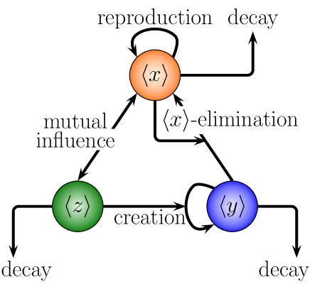
Figure 1: (Color online) Schematic illustration of the model presented in Eq. (13).

Let us compare the results of the stochastic approach with the deterministic model. The birth rate of the tumor cells $\langle x\rangle$ are affected by the noise correlation strengths $D_{x}$, $D_{z}$ associated with the tumor cells and the tumor detecting cells as well as their cross-correlation $R$. Likewise the decay rate $\rho$ in the equation for the effector cells $\langle y\rangle$ is reduced by the noise strength $D_{y}$, i.e. by the noise related to the effector cell subsystem itself. As a new nontrivial result we find noise induced terms in the evolution equation Eq. (13). So there appears a term $\propto\langle x(t)\rangle$ in the equation for the $z$-cells which are able to recognize cancer cells. In the same manner the generating term $\propto\langle z(t)\rangle$ arises in the equation for the tumor cells. These terms are originated exclusively due to the randomness in Eqs. (4) and (5). In this context the most important parameter is played by the cross correlation strength $R$ of the correlation function $\chi_{xz}=\chi_{zx}$, i.e. the correlation between the noise sources inherent in the tumor cells and the tumor detecting cells. Notice that in the noise-free case such an interlink between these two cells is missing, compare again Fig. 1. Moreover, the death rate $\mu$ is altered due to the stochastic process. Based on the implementation of noisy forces the resulting Eq. (13) differs from the deterministic equation twice. (i) Firstly, the birth and death rates as well are altered due to stochastic parameters such as the correlation time $\tau$ and the correlation strengths $D_{x}$, $D_{y}$, $D_{z}$ and $R$ defined in Eq. (7). Although the cross-correlations $S$ and $P$ were included in Eqs. (4) and (5), they do not appear in the final expression Eq. (13). This fact is related to the special kind of multiplicative noise of our model. (ii) Secondly, two new terms exist in Eq. (13). The origin of both can be solely ascribed to stochastic sources. Regarding the evolution of the tumor detecting cells $\langle z\rangle$ the new term disappears in case $R=0$ and $\tau=0$. So both parameters $R$ -the cross-correlation strength between $\eta_{x}$ and $\eta_{z}$ and $\tau$ -the correlation time of the auto-correlation functions $\langle\eta_{i}(t)\eta_{i}(t^{\prime})\rangle$- are of significant relevance. In the subsequent section the analysis is focused in particular on both parameters.

V Results and discussion

As remarked in the previous section the parameters $R$ and $\tau$ inhere a special meaning in discussing the set of Eq. (13). Before we proceed with the stability analysis and the results we want to estimate the model parameters. The starting point is the deterministic Eq. (1). One finds different values for the intrinsic tumor growth rate $a$: $0.18~{}\rm{day}^{-1}$ Kuznetsov:BullMathBiol:56:1994 and $0.51~{}\rm{day}^{-1}$ DePillis:CancerRes:65:7950:2005 . Our own study leads to $0.57~{}\rm{day}^{-1}$ BoseTrimper:PRE:2009:051903 . The first two values are based on mouse models while the latter one was obtained by means of in vitro cultivation of tumor cells. The growth rate is insofar of importance as it determines the time scale of the dynamics, see Eq. (3) ($t~{}[\rm{in\,days}]=\bar{t}/a$). Here we use $a=0.5~{}\rm{day}^{-1}$. Thus, $\bar{t}=1$ is tantamount to $t=2~{}\rm{days}$. An estimation of the carrying capacity is $b^{-1}=10^{9}~{}\rm{cells}$ Kuznetsov:BullMathBiol:56:1994 ; DePillis:CancerRes:65:7950:2005 . Further, the reaction rates take approximately $c=10^{-7}~{}\rm{cell}^{-1}~{}\rm{day}^{-1}=e$ Kuznetsov:BullMathBiol:56:1994 ; DePillis:CancerRes:65:7950:2005 ; KirschnerPanetta:JMathBiol:1998 ; Rodriguez-P:MathMedBiol:24:2007 . An estimation for the decay rates in Eq. (1) is given by $\tilde{\rho}=3\times 10^{-2}~{}\rm{day}^{-1}$ and $\tilde{\mu}=10~{}\rm{day}^{-1}$ DePillis:CancerRes:65:7950:2005 ; KirschnerPanetta:JMathBiol:1998 . In relating our results to real units one should take into account the scaling properties Eq. (3). All the results are collected at the end of this section in Tab. 1. For the subsequent analysis it is more convenient to use dimensionless quantities. The both most relevant parameters of stochastic forces are the auto-correlation time $\tau$ and the cross-correlation strength $R$. Both quantities $R$ and $\tau$ will be altered within the interval $[0,5]$. The remaining parameters are assumed to be fixed, i.e. $D_{x}=2.1$, $D_{z}=1.2$ and $D_{y}=0.01$. The values for $D_{x}$ and $D_{z}$ are chosen arbitrarily, whereas the value for $D_{y}$ is suggested to be smaller than $\rho=\tilde{\rho}/a=0.06$ in order to guarantee a sufficient stability of the differential equation system Eq. (13), cf. the term $\propto\langle y\rangle$. Moreover, since we consider cell populations the solutions of Eq. (1) should yield positive values for the cell numbers. So values of $R$ and $\tau$ are excluded when they induce negative values for the cell populations.

Now we perform the stability analysis according to the tumor-immune cells reaction system satisfying Eq. (13). We note that the numerical bifurcation analysis is performed by means of the program xppaut541 which contains the bifurcation tool autobif . This set of equations exhibits three different equilibria, i.e. the tumor-free $E_{1}=(0,0,0)$, and two non-tumor-free states designated as $E_{2}$ and $E_{3}$. The last ones are given by lengthy expressions in terms of the model parameters. Only one of the three equilibria is stable simultaneously. It is also possible that the total system becomes unstable as discussed below. The solution of Eq. (13) depends strongly on the correlation time $\tau$ and the cross-correlation strength $R$. Concerning $\tau$ we find three different regions (labeled as I-III) where the solution of Eq. (13) has different properties. The threshold values referring to our specific numerical values of the remaining model parameters are $\tau_{c_{1}}=0.636$ and $\tau_{c_{2}}=4.016$. We proceed by considering these three regions determined by the correlation time $\tau\in[0,5]$. As fixed initial values for the tumor and the tumor detecting cells, respectively, we choose $\langle x(t=0)\rangle=10^{-6}$ and $\langle z(t=0)\rangle=0$ . This reflects a situation where the tumor is small and tumor detecting cells are not present. In our case this equals an initial tumor cell number of $10^{3}~{}\rm{cells}$ which is clinically not detectable (early stages of tumor evolution).

(a)  $\tau=0.3\to$ region I

(b)  $\tau=2.0\to$ region II

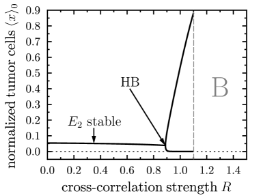
(c)  $\tau=4.5\to$ region III

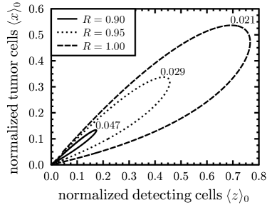
(d)  $\tau=4.5\to$ region III

Figure 2: Behavior of the solution representing the regions I-III mentioned in the text. The parameters take $\rho=0.06$, $\mu=20$, $D_{x}=2.1$, $D_{y}=0.01$ and $D_{z}=1.2$. (a)-(c): Bifurcation diagrams. (d) Limit cycles in the $\langle x\rangle-\langle z\rangle-$pahse space.

Tumor detecting cells should be only generated due to stochastic influences and did not exist a priori. For the initial state of the effector cell population we have to choose a non-zero value of $\langle y(t=0)\rangle>0$. Otherwise the solution will differ from the predictions based on the stability analysis which is due to the structure of the differential equation system in Eq. (13). In some regions this value can be very small (almost zero, e.g. $\sim 10^{-20}$) whereas in other areas corresponding to the parameters $R$ and $\tau$ the stability of the solution depends on $\langle y(t=0)\rangle$ significantly . In what follows these distinct cases will also be discussed while we want to restrict the possible values for $\langle y(t=0)\rangle$ to the left-open interval $(0,10]$.

Region I ($0\leq\tau\leq\tau_{c_{1}}=0.636$): Within this range a stable tumor-free state is missing for $R\in[0,5]$. All three fixed points exist in this region. The solution tends either to the steady states $E_{2}$ or $E_{3}$ one of which is asymptotically stable which depends on the cross-correlation strength $R$. For instance in case of $\tau=0.3$ the equilibrium value of the tumor cell population, designated as $\langle x\rangle_{0}$ as a function of $R$, is depicted in Fig. 2(a). As is visible for all $0\leq R\leq 5$ the solution will always reach the fixed point $E_{2}$. Further, the equilibrium value $\langle x\rangle_{0}$ decreases with increasing $R$. In region I the initial value of the effector cells can take arbitrary positive values in $(0,10]$ without changing the solution of Eq. (13). An exemplary dynamical solution is illustrated in Fig. 3(a).

Region II ($\tau_{c_{1}}=0.636<\tau<\tau_{c_{2}}=4.016$): In this area the behavior is changed and one observes diagrams like that one shown in Fig. 2(b) for $\tau=2.0$. The three fixed points $E_{1,2,3}$ survive for $R\in[0,5]$, but the stability is changed. If we start at $R=0$ and increase the cross-correlation strength $R$ the behavior of the solution traverses four different regions. For $0\leq R<1.242$ the steady state $E_{2}$ is stable. At $R=1.242$ a transcritical bifurcation occurs where $E_{2}$ is not stable anymore. The fixed point $E_{3}$ becomes stable but only within the interval $1.242\leq R<1.325$. At $R=1.325$ another transcritical bifurcation occurs namely the transition to the tumor-free state $E_{1}$ which becomes stable while $E_{3}$ loses its stability. Biologically such a transition is of great relevance because it manifests that the immune system is able to eliminate a growing tumor provided the tumor-immune cells reaction is assisted by a cross-correlation between stochastic events occurring in the tumor and in the tumor detecting cells subsystem. Notice that the sector A in Fig. 2(b) has to be excluded because the eigenvalues of $E_{1}=(0,0,0)$ develop an imaginary part indicating the solution tends to $E_{1}$ on a stable spiral. However, during the evolution towards the equilibrium value ($\langle x(t)\rangle\to\langle x\rangle_{0}$, $t\to\infty$) the tumor cell population $\langle x(t)\rangle$ takes negative values. This happens for $R>1.733$ which is indicated by the sector A in Fig. 2(b). In the area $R\leq 1.733$ there are no restrictions on the initial value for the effector cells $0<\langle y(0)\rangle\leq 10$. In Fig. 3(b) the time evolution of the tumor cell number $\langle x(t)\rangle$ is shown for different values of the cross-correlation strength $R$. Summarizing the result we observe in region II the occurrence of tumor escape as well as the possibility of tumor elimination depending on the value of the cross-correlation strength $R$.

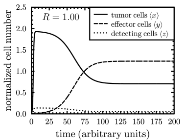
(a)  $\tau=0.3\to$ region I

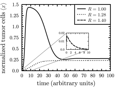
(b)  $\tau=2.0\to$ region II

(c)  $\tau=4.5\to$ region III

(d)  $\tau=4.5\to$ region III

Figure 3: Exemplary dynamic solutions according to the regions I-III mentioned in the text. The parameters take $\rho=0.06$, $\mu=20$, $D_{x}=2.1$, $D_{y}=0.01$ and $D_{z}=1.2$.

Region III ($\tau_{c_{2}}=4.016\leq\tau\leq 5$): In this parameter range one observes a new behavior determined by the cross-correlation strength $R$ and the initial value of the effector cells $\langle y(0)\rangle$. For the following discussion we refer to Fig. 2(c). Starting from $R=0$ and increasing this parameter the solution of Eq. (13) tends to the stable fixed point $E_{2}$. A related solution is represented in Fig. 3(c), where it needs a rather long time until $E_{2}$ is reached, about $t\sim 19000$. The fixed point $E_{2}$ is realized on a stable spiral within the interval $0\leq R<0.888$. The smaller the cross-correlation strength $R$ is the shorter is the time scale to reach $E_{2}$, for instance we need $t=1000$ in case $R=0.01$. When the critical value $R=0.888$ is exceeded a periodic limit cycle evolves related to the occurrence of a Hopf bifurcation. In Fig. 2(c) the minimal and the maximal numbers of tumor cells are plotted within such a limit cycle. The numerical values range below and above the former stable equilibrium $E_{2}$ which becomes now unstable. After the Hopf bifurcation the steady states $E_{1}$ and $E_{3}$ are no longer detectable. Further, Fig. 2(c) reveals that the the parameter range is limited in which such stable periodic oscillations emerge. The dashed line represents the boundary to sector B, where the total system bifurcates into an unstable state and the dynamical system is uncontrollable anymore. Thus the sector B will be excluded as a domain of accessible solutions within our tumor-immune model. Nevertheless, periodic orbits can be observed for $0.888\leq R\leq 1.101$ and fixed correlation time $\tau=4.5$. For varying values of $R$ the periodic solutions are depicted in the two-dimensional $\langle x\rangle-\langle z\rangle-$phase space, see Fig. 2(d). The numbers shown above each orbit is the frequency of the oscillations between two maxima. With growing $R$ from $0.9$ to $1.0$ the minimal and the maximal cell numbers increase for both $\langle x\rangle$ and $\langle z\rangle$ while the frequency decreases, i.e. the period of the oscillation is enlarged. This result is also valid for the effector cells $\langle y\rangle$ which are not shown here.

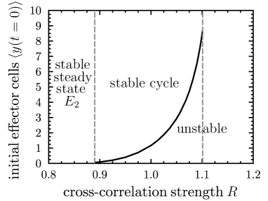
Figure 4: Distinction between stable and unstable solutions depending on $\langle y(0)\rangle$ and $R$. Further description in the text.

Coming back to the influence of the initial values of the effector cells $\langle y(0)\rangle$. As already mentioned they play a decisive role in the regime of periodic limit cycle solutions. For very low initial values the system loses its stability and the solution is not accessible biologically. The curve which separates stable periodic cycles from unstable solutions is displayed in Fig. 4. The question arises what does it means for the real tumor-immune cells interactions if stable periodic oscillations occur? In that case we argue that an intensive interaction between the cancer and the immune cells takes place at the beginning of the tumor growth as well as after a long period later. If the nascent transformed cells start to grow up the immune system is able to detect this harmful process and it responds. Such an immune attack reduces the tumor size without to delete it completely. Notice that our numerical estimation represented in Fig. 2(c) is also compatible with an elimination of the tumor cells because the lower branch is partly not distinguishable from zero in the interval $0.888\leq R\leq 1.101$. But the tumor starts anew to grow up signalizing the latent facility that the tumor evolution goes on. Otherwise, if the cancer growth is continued the immune system remains active and consequently it is still able to eliminate a large amount of tumor cells. So after a certain time one expect that a balance between tumor growth and the response of the immune system is evolved. From here one concludes that the tumor is under the control of the immune system and a so called tumor dormant state emerges. In the same manner the region with $R<0.888$ (before the Hopf bifurcations appears) may also be interlinked to the tumor dormant state. In that case the number of tumor cells is low compared to other parameter regimes, see Fig. 2. For instance the value $R=0.6$ yields an equilibrium tumor cell population of $5\%$ of the carrying capacity in Fig. 2(c). However, as a result of our computations, the size of the maximal number of tumor cells within one cycle can take large values, e.g. for $R=1.1$ we find $\langle x\rangle_{max}=0.88$. The tumor reaches $88\%$ of its carrying capacity. The time-dependent solution for $R=1.0$ is depicted in Fig. 3(d) within the interval $0\leq t\leq 500$. Eventually a periodic cycle with $\langle x\rangle_{max}=0.54$ will be reached after $t\sim 12000$.

At the end of this section we want to convert some dimensionless quantities into quantities with real units. The results are particularized in Tab. 1.

quantity	arbitrary units	real units
time t	$1$	$2~{}\rm{days}$
auto-correlation time $\tau$	$1$	$2~{}\rm{days}$
cross-correlation strength $R$	$1$	$0.5~{}\rm{day^{-1}}$
number of tumor cells $\langle x\rangle$	$1$	$10^{9}~{}\rm{cells}$
number of effector cells $\langle y\rangle$	$1$	$5\times 10^{6}~{}\rm{cells}$
number of tumor detecting cells $\langle z\rangle$	$1$	$5\times 10^{6}~{}\rm{cells}$
frequency (period) of cycles	$0.029$	$\approx 0.01~{}\rm{day}^{-1}$
according to Fig. 2(d)	($\approx 34.5$)	($\approx 69~{}\rm{days}$)

Table 1: Comparison of model quantities in arbitrary and real units. See also Eq. (3).

Not commented yet is that the strengths in the correlation functions in Eq. (6) carry the unit $\rm{day}^{-1}$ after conversion to real units. This follows from the correlation function in real units, i.e. $\langle\eta_{i}\eta_{j}^{\prime}\rangle\,a^{2}\propto(D_{ij}\,a)/(\tau_{ij}/a)$ where the intrinsic tumor growth rate $a=0.5~{}\rm{day^{-1}}$ and $D_{ij}$ and $\tau_{ij}$ are given in arbitrary units. Thus, the strengths occurring in the noise-noise correlation functions in Eq. (6) have the meaning of a rate.

VI Conclusions

We have presented a mathematical model for the tumor-immune cells reactions which is essentially supplemented by stochastic forces. The parameters of the noise correlation function have a great impact on the behavior of the coupled tumor-immune cell interaction, especially on the response of the immune system. In particular we have emphasized that the auto-correlation time $\tau$ and the cross-correlation strength $R$ are able to control the evolution of the tumor. More precise, these two quantities discriminate whether the system tends to tumor suppression, tumor progression or tumor dormancy. The assistance of an inevitable noisy influences seems to play a crucial role during cancer genesis and growth in humans. The involved random forces may be originated within the tumor as well as inside the immune system and can even interact mutually which is manifested in the cross-correlation. Our model should be considered as an attempt toward a more detailed analysis of tumor-immune systems. But also the model studied elucidates that noise plays an decisive role in such systems. The model can be refined immediately, e.g. a finite correlation time is attributed to the cross-correlation functions, too. In that case the correlation time matrix, Eq. (7), is modified and new terms in Eq.(13) occur. We believe that our approach includes the most relevant degrees of freedom.

One of us (T.B.) is grateful to the Research Network ’Nanostructured Materials’ , which is supported by the Saxony-Anhalt State, Germany.

References

- (1) V. Kuznetsov, I. Makalkin, M. Taylor, and A. Perelson, Bull. Math. Biol. 56, 295 (1994)
- (2) D. Kirschner and J. C. Panetta, J. Math. Biol. 37, 235 (1998)
- (3) V. A. Kuznetsov and G. D. Knott, Math. Comput. Modell. 33, 1275 (2001)
- (4) L. G. DePillis, A. E. Radunskaya, and C. L. Wiseman, Cancer Res. 65, 7950 (2005)
- (5) D. Rodríguez-Pérez, O. Sotolongo-Grau, R. Espinosa Riquelme, O. Sotolongo-Costa, J. A. Santos Miranda, and J. C. Antoranz, Math. Med. Biol. 24, 287 (2007)
- (6) J. D. Murray, Mathematical Biology (Springer, Berlin, 1993)
- (7) M. Khasin and M. I. Dykman, Phys. Rev. E 83, 031917 (2011)
- (8) M. Ben Amar, C. Chatelain, and P. Ciarletta, Phys. Rev. Lett. 106, 148101 (2011)
- (9) A. J. Bladon, T. Galla, and A. J. McKane, Phys. Rev. E 81, 066122 (2010)
- (10) M. Parker and A. Kamenev, Phys. Rev. E 80, 021129 (2009)
- (11) M. Assaf and B. Meerson, Phys. Rev. E 81, 021116 (2010)
- (12) T. Bose and S. Trimper, Phys. Rev. E 79, 051903 (2009)
- (13) G. Aquino, M. Bologna, and H. Calisto, Europhys. Lett. 89, 50012 (2010)
- (14) A. Di Garbo, M. D. Johnston, S. J. Chapman, and P. K. Maini, Phys. Rev. E 81, 061909 (2010)
- (15) B.-Q. Ai, X.-J. Wang, G.-T. Liu, and L.-G. Liu, Phys. Rev. E 67, 022903 (2003)
- (16) A. d’Onofrio, Phys. Rev. E 81, 021923 (2010)
- (17) P. Ehrlich, Ned. Tijdschr. Geneeskd. 5 5, 273 (1909)
- (18) F. M. Burnet, Brit. Med. J. 1, 841 (1957)
- (19) L. Thomas, Cellular and Humoral Aspects of the Hypersensitive States (Hoeber-Harper, 1959)
- (20) V. Shankaran, H. Ikeda, A. T. Bruce, J. M. White, P. E. Swanson, L. J. Old, and R. D. Schreiber, Nature 410, 1107 (2001)
- (21) G. P. Dunn, A. T. Bruce, H. Ikeda, L. J. Old, and R. D. Schreiber, Nat. Immunol. 3, 991 (2002)
- (22) R. Kim, M. Emi, and K. Tanabe, Immunology 121, 1 (2007)
- (23) R. D. Schreiber, L. J. Old, and M. J. Smyth, Science 331, 1565 (2011)
- (24) D. Hanahan and R. A. Weinberg, Cell 144, 646 (2011)
- (25) K. Schroder, P. J. Hertzog, T. Ravasi, and D. A. Hume, J. Leuk. Biol. 75, 163 (2004)
- (26) L. Wall, F. Burke, C. Barton, J. Smyth, and F. Balkwill, Clin. Cancer Res. 9, 2487 (2003)
- (27) C. W. Gardiner, Handbook of Stochastic Methods for Physics, Chemistry and the Natural Sciences (Springer, 1990)
- (28) N. G. van Kampen, Stochastic Processes in Physics and Chemistry (North-Holland, Amsterdam, 1981)
- (29) E. A. Novikov, Sov. Phys. JETP 20, 1290 (1965)
- (30) R. F. Fox, J. Math. Phys. 18, 2331 (1977)
- (31) L. Garrido and J. M. Sancho, Physica A: Statistical and Theoretical Physics 115, 479 (1982)
- (32) H. Dekker, Phys. Lett. A 90, 26 (1982)
- (33) A. Hernandez-Machado, J. M. Sancho, M. San Miguel, and L. Pesquera, Zeitschr. f. Phys. B 52, 335 (1983)
- (34) G. B. Ermentrout, XPPAUT5.41 - the differential equation tool(2003), http://www.pitt.edu/~phase/
- (35) E. Doedel, AUTO - software for continuation and bifurcation problems in ordinary differential equations(1980-2011), http://indy.cs.concordia.ca/auto/