Bounds on the capacity of OFDM underspread frequency selective fading channels

Abstract

The analysis of the channel capacity in the absence of prior channel knowledge (noncoherent channel) has gained increasing interest in recent years, but it is still unknown for the general case. In this paper we derive bounds on the capacity of the noncoherent, underspread complex Gaussian, orthogonal frequency division multiplexing (OFDM), wide sense stationary channel with uncorrelated scattering (WSSUS), under a peak power constraint or a constraint on the second and fourth moments of the transmitted signal. These bounds are characterized only by the system signal-to-noise ratio (SNR) and by a newly defined quantity termed effective coherence time. Analysis of the effective coherence time reveals that it can be interpreted as the length of a block in the block fading model in which a system with the same SNR will achieve the same capacity as in the analyzed channel. Unlike commonly used coherence time definitions, it is shown that the effective coherence time depends on the SNR, and is a nonincreasing function of it.

We show that for low SNR the capacity is proportional to the effective coherence time, while for higher SNR the coherent channel capacity can be achieved provided that the effective coherence time is large enough.

I Introduction

The analysis of communication systems is often performed under the assumption of perfect channel knowledge. In practical systems, however, the channel needs to be estimated from the communication signal itself, making this assumption unrealistic.

In this paper we study the capacity of the noncoherent, underspread, complex Gaussian, orthogonal frequency division multiplexing (OFDM), wide sense stationary channel with uncorrelated scattering (WSSUS), under a peak power constraint or a constraint on the second and fourth moments of the transmitted signal (commonly termed quadratic power constraint). We use the term noncoherent channel capacity to describe the capacity of the channel when neither the transmitter nor the receiver have any prior knowledge on the channel realization, but both have exact knowledge on the channel statistics.

The OFDM model provides a simple representation of an underspread frequency selective channel [1]. In underspread channels the channel delay spread is significantly smaller than the channel coherence time [2]. Choosing the OFDM symbol length to be significantly larger than the channel delay spread, and yet significantly smaller than the channel coherence time, results in a useful approximation of the underspread channel which is both accurate and convenient for the analysis. (Detailed description on the connection between the OFDM model and the general WSSUS channel can be found in [3, 4].)

This paper presents novel bounds on the capacity of the noncoherent underspread WSSUS channel that are characterized only by the system signal-to-noise ratio (SNR) and by a newly defined quantity termed effective coherence time. We show that the bounds are good for almost all of the SNR range as long as the effective coherence time is significantly larger than the OFDM symbol length. Analysis of the effective coherence time reveals that it characterizes the system ability to estimate the channel, and can be interpreted as the length of a block in the block fading model that achieves the same capacity as the analyzed channel at the same SNR. Surprisingly, and unlike standard coherence time definitions, the effective coherence time is actually a function of the system SNR. This dependence of the effective coherence time on SNR stems from the fact that at high SNR the system is more sensitive to changes in the channel, and hence will effectively see a shorter coherence time. The paper also includes a detailed study of the relation between the effective coherence time and the system SNR.

The noncoherent underspread WSSUS channel capacity was well characterized for the high SNR limit and for the low SNR limit (which is equivalent to the large bandwidth limit). For the low SNR limit, the capacity of the noncoherent underspread channel was shown to be proportional to $p_{x}^{2}{T_{\rm c}}/2$, where $p_{x}$ is the SNR and ${T_{\rm c}}$ is the channel coherence time [3]–[7]. These results were obtained for different channel models with different constraints. Medard and Gallager [5] analyzed a stationary wideband channel with quadratic power constraint, and presented a novel definition of the channel coherence time which is calculated from the channel correlation function. In this case, the proportionality constant is the ratio between the transmitted signal fourth moment and the square of its second moment (also termed Kurtosis). The results in that work were derived for the wide bandwidth limit (in which the capacity depends on the number of resolvable channel taps, see also [8, 9]). In this paper, the channel bandwidth is finite, and we address the above result only in its low SNR limit interpretation.

Sethuraman and Hajek [6] considered the block fading model with a peak power constraint. In that case the channel coherence time is the length of a block, and the proportionality constant was shown to be the ratio between the peak and average powers. They also considered a flat fading stationary channel model (i.e., without multipath spread) and achieved equivalent results, but using measures of the channel spectral distribution function (with no definition of channel coherence time). In a later work together with Wang and Lapidoth [7], they considered delay-separable frequency selective fading channels, and showed that the capacity is actually proportional to $p_{x}^{2}({T_{\rm c}}-1)/2$; here the definition of the channel coherence time is the identical to the one used by Medard and Gallager [5] but the term coherence time is not used. (Note that for underspread channels the difference between ${T_{\rm c}}$ and ${T_{\rm c}}-1$ is negligible.)

Durisi et al. used a similar channel model, but paid more attention to the discretization of the continuous time channel (and did not require the channel to be delay separable). As a result, they had worked with a time-frequency channel transfer function (which resembles in nature to the OFDM model used herein). They also did not use the term coherence time, but their results revealed the same behavior of the capacity in the low SNR limit, using a channel measure which is an extension of Medard and Gallager [5] coherence time to the time-frequency channel. (In their work they also analyzed the capacity with per frequency peak power constraint. This power constraint is not discussed herein, as it is quite different and leads to a significantly different capacity behavior.)

For the high SNR limit, the main issue is whether the channel estimation error can decrease to 0 as the SNR grows to infinity. The channel fading is termed regular if it cannot be completely predicted based on the full knowledge of its past [10]. An alternative definition uses the covariance matrix of the channel fading, and the channel is said to be regular if this matrix is full rank [11]. For regular channels, at high enough SNR, the capacity in the absence of channel knowledge is significantly lower than the capacity with perfect channel knowledge, and grows only double logarithmically with SNR [12, 13, 14]. On the other hand, for irregular channels the capacity can continue to grow logarithmically with SNR, (with possible degradation in the pre log constant) [13, 14].

Interestingly, no capacity expression directly depends on the common definition of coherence time (e.g., [15]), i.e., the inverse of the channel Doppler spread. For stationary channels, the only coherence time definition that was shown to be proportional to the capacity is the one given by Medard and Gallager [5], which only applies in the low SNR limit. The definition of effective coherence time in this paper coincides with Medard’s and Gallager’s coherence time definition in the low SNR limit, and extends it to higher SNR. Thus, the effective coherence time can characterize the channel capacity for all SNRs.

The paper is organized as follows: the notation and channel model are presented in Sections II and III respectively. The main results, including the definition of the effective coherence time and the capacity bounds are given in Section IV. A discussion of the results including the properties of the effective coherence time, analysis of the bounding gap, numerical examples and comparison to known results are given in Section V. Note that the proof of each of the theorems (providing capacity bounds) is partly based on information theory and partly on estimation theory. For convenience, we collect those parts in different sections. Hence, Theorem $n$ ($n=1,2,3$) is proved by lemma $n$.a in Section VI (information theory part) and lemma $n$.b in Section VII (estimation theory part). Concluding remarks are given in Section VIII.

II Notation

Throughout the paper we use Roman boldface lower case and upper case letters to denote random scalars and vectors, respectively (e.g., ${\bf x}$, ${\bf X}$). Roman italic lower case and upper case letters are used for deterministic scalars and vectors, respectively (e.g., $x$, $X$). Deterministic matrices are represented by sans-serif letters and random matrices by calligraphic letters (e.g., X, $\cal{X}$ ). Exceptions to this rule are scalar quantities that are commonly denoted by uppercase letters. These include the channel parameters $N$ and $L$, the coherence time symbol (${T_{\rm c}}$, ${\hat{T}_{{\rm c}}}(\cdot)$ and ${\hat{T}_{{\rm c}_{0}}}$), and the capacity symbol $C$. Another exception are operators that can result in a deterministic or random quantity according to their operand, i.e., the spectrum operator ${\mathcal{S}}_{\cdot}$ (see definition below) and the symbol set operator $\mathcal{I}(\cdot)$ (see definition in Lemma 1.b).

The identity matrix is denoted by I, ${\rm 0}_{N}$ and ${\rm 1}_{N}$ denote the $N\times 1$ vectors of all zeros and all ones, respectively. A $\otimes$ symbolizes the Kronecker product, a $\dagger$ stands for transposition and complex conjugation, $\left\|\textsf{A}\right\|$ denotes the absolute value of the determinant of the matrix A, and ${\rm diag}({X})$ is the diagonal matrix with the elements of the vector ${X}$ on its diagonal. The vector stacking is defined as: ${X}_{k}^{n}\triangleq[{X}_{k}^{T},\ldots,{X}_{n}^{T}]^{T}$. The $b,d$ element of a matrix A is denoted as $(\textsf{A})_{b,d}$ and the $b$-th element of the vector $X_{k}$ is denoted as $x_{k,b}$.

For discrete Fourier transform (DFT) analysis, ${\sf{F}}$ denotes the DFT matrix with elements:

$${\sf{F}}_{m,n}=\frac{1}{{\sqrt{N}}}e^{-2j\pi mn/N},$$ (1)

$\tilde{X}={\sf{F}}^{\dagger}{X}$ denotes the DFT of a vector, and each element in this vector is termed a frequency bin. The spectrum of a vector is marked by:

$${\mathcal{S}}_{X}={\rm diag}(\tilde{X}){\rm diag}(\tilde{X})^{\dagger}.$$ (2)

The cross-covariance matrix of the vectors $\bf X$ and $\bf Y$ is denoted as:

$${\sf C}_{{\bf X},{\bf Y}}=E\left[\left({\bf X}-E[{\bf X}]\right)\left({\bf Y}-E[{\bf Y}]\right)^{\dagger}\right],$$ (3)

and the auto-covariance matrix of the vector ${\bf X}$ is denoted as ${\sf C}_{{\bf X}}={\sf C}_{{\bf X},{\bf X}}$.

Finally, any matrix ordering in this paper is in the positive definite sense, i.e., $\textsf{A}\geq\textsf{B}$ means that $\textsf{A}-\textsf{B}$ is positive semi-definite.

III System model

III-A Channel model

We use the OFDM model [1, 4, 16, 17], in which the DFT of the received signal is given by:

$${{\tilde{\bf{Y}}_{k}}} = \sqrt{N}{\rm diag}({{\tilde{\bf{H}}_{k}}}){{\tilde{\bf{X}}_{k}}}+{{\tilde{\bf{W}}_{k}}}$$ (4)

$$= \sqrt{N}{\rm diag}({{\tilde{\bf{X}}_{k}}}){{\tilde{\bf{H}}_{k}}}+{{\tilde{\bf{W}}_{k}}}$$

where ${\tilde{\bf{X}}_{k}}\triangleq{\sf{F}}^{\dagger}{{\bf{X}}_{k}}$ and ${\tilde{\bf{H}}_{k}}\triangleq{\sf{F}}^{\dagger}{{\bf{H}}_{k}}$ are the DFT of the input vector and channel impulse response at the $k$-th symbol respectively, and both are vectors of length $N$. Each input vector constitutes an OFDM symbol. The frequency domain noise ${\tilde{\bf{W}}_{k}}\triangleq{\sf{F}}^{\dagger}{{\bf{W}}_{k}}$ is a zero mean complex Gaussian vector with covariance matrix: ${{{\sf{C}}_{{\bf{\tilde{W}}}}}}={{\textsf{I}}}$. The multiplication by $\sqrt{N}$ follows from the definition of the DFT matrix, (1). The channel itself is better characterized in the time domain where ${{\bf{H}}_{k}}=[{{\bf{h}}_{k,0}},\ldots,{{\bf{h}}_{k,L-1}},0,\ldots,0]^{T}$, and $L$ is termed the channel delay spread.

This model is an appropriate representation of an underspread channel in which we assume ${T_{\rm c}}\gg N\gg L-1$, where ${T_{\rm c}}$ is the channel coherence time [15]. The assumption guarantees that the channel Doppler spread is small enough to be negligible, and that the channel impulse response can be considered constant throughout the $N$ samples that constitute an OFDM symbol (for analysis of faster fading channels see [18]). The small channel delay spread, $L$, permits to neglect the time required for cyclic prefix ($L-1$ samples after each OFDM symbol).

In Section IV we define a new parameter, the effective coherence time, ${\hat{T}_{{\rm c}}}(p_{x})$, which identifies the effective number of received samples that can be used for channel estimation. The impact of the effective coherence time on the channel capacity will be treated in later sections.

The mathematical analysis in the paper requires the following assumptions:

Assumption I

The channel is underspread, i.e., the channel coherence time and the effective coherence time (measured in channel samples) are large enough so that: ${T_{\rm c}},{\hat{T}_{{\rm c}}}(p_{x})\gg N$.

Assumption II

The channel has a proper complex Gaussian distribution ([19]).

Assumption III

The transmitter has no knowledge on the channel realization.

Assumption IV

The channel is ergodic, (wide sense) stationary, with uncorrelated scattering (WSSUS channel).

Assumption V

The auto-correlation function of the different channel taps is identical up to a multiplication by a scalar.

Assumption VI

The expectation of the channel impulse response is frequency flat.

Assumption I is actually not needed for the analysis presented herein. We state it as our first assumption because it is the basis for the OFDM model. If the coherence time is not significantly larger than the symbol length, then our model, which implicitly assumes that the channel does not change during an OFDM symbol, will not be realistic.

Assumption III stems from the fact that the system has no feedback. As a result, the transmitted messages are statistically independent from the channel. The requirement of uncorrelated scattering in Assumption IV is needed mostly for low SNR where we show that it is better to concentrate the transmission power in a single frequency bin. The uncorrelated scattering guarantees that if in one OFDM symbol we transmit in a certain frequency bin, the best channel estimate for the next OFDM symbol will be achieved at the same frequency bin (see derivation in Appendix B).

Assumptions V and VI somewhat narrow the scope of the analysis. However, we keep them to simplify the mathematical derivation, and to reach closed-form expressions. Assumption V, although not necessarily realistic, is common to many simple channel models (e.g., assuming that all multipath components have identical doppler spread). Channels that satisfy this assumption are sometimes referred to as delay separable channels [7]. Assumption VI basically states that at most one channel tap has an expectation different from zero, and it includes the case of Rayleigh fading (the expectation is zero) and the case of line of sight (LOS) propagation (one channel tap has an expectation different from zero).

Using Assumption II, the stacking of the channel vector has a proper complex Gaussian distribution, ${{\bf{H}}_{0}^{k}}\sim\mathcal{CN}(E[{{\bf{H}}_{0}^{k}}],{\sf C}_{{{\bf{H}}_{0}^{k}}})$. Using Assumption IV the amplitudes of the different channel taps (in the time domain, ${{\bf{h}}_{k,0}},\ldots,{{\bf{h}}_{k,L-1}}$) are statistically independent. Using also Assumption V the covariance matrices of the channel taps are identical up to a multiplication by a scalar. Considering $k+1$ OFDM symbols, we denote by $\Delta_{k}$ the single-tap $(k+1)\times(k+1)$ Toeplitz covariance matrix, in which each element is given by

$$({{\Delta}_{k}})_{i,j}={{\sf C}_{{{\bf{h}}_{i,0}},{{\bf{h}}_{j,0}}}}/{{\sf C}_{{{\bf{h}}_{0,0}}}}.$$ (5)

We also define the $k\times 1$ vector ${{D}_{k}}$ in which the $i$-th element is given by

$${d}_{k,i}=({{\Delta}_{k}})_{i,k},\quad i=0,\ldots,k-1.$$ (6)

This vector is the correlation between the channel tap value at the $k$-th symbol and its value at all previous symbols. Considering all channel taps, the covariance matrix of the stacked channel vector ${{\bf{H}}_{0}^{k}}$ is:

$${\sf C}_{{{\bf{H}}_{0}^{k}}}={{{\Delta}_{k}}}\otimes{\sf{C}}_{{{\bf{H}}_{0}}}=\left(\begin{IEEEeqnarraybox}[]{[}][c]{c?c?c?c}({{\Delta}_{k}})_{0,0}{\sf{C}}_{{{\bf{H}}_{0}}}&({{\Delta}_{k}})_{0,1}{\sf{C}}_{{{\bf{H}}_{0}}}&\ldots&({{\Delta}_{k}})_{0,k}{\sf{C}}_{{{\bf{H}}_{0}}}\\ ({{\Delta}_{k}})_{1,0}{\sf{C}}_{{{\bf{H}}_{0}}}&({{\Delta}_{k}})_{1,1}{\sf{C}}_{{{\bf{H}}_{0}}}&\ldots&({{\Delta}_{k}})_{1,k}{\sf{C}}_{{{\bf{H}}_{0}}}\\ \vdots&\vdots&\ddots&\vdots\\ ({{\Delta}_{k}})_{k,0}{\sf{C}}_{{{\bf{H}}_{0}}}&({{\Delta}_{k}})_{k,1}{\sf{C}}_{{{\bf{H}}_{0}}}&\ldots&({{\Delta}_{k}})_{k,k}{\sf{C}}_{{{\bf{H}}_{0}}}\end{IEEEeqnarraybox}\right),$$ (11)

and ${\sf{C}}_{{{\bf{H}}_{0}}}$ is an $N\times N$ diagonal matrix, in which each diagonal element represents the power of one channel tap (note that due to Assumption IV, we can write ${\rm{C}}_{{{\bf{H}}_{k}}}={\sf{C}}_{{{\bf{H}}_{0}}}$ for any $k$). In the following we mostly consider the frequency domain channel, ${\tilde{\bf{H}}_{k}}={\sf{F}}^{\dagger}{{\bf{H}}_{k}}$. Its covariance matrix is given by ${\sf C}_{{\tilde{\bf{H}}_{k}}}={\sf{F}}^{\dagger}{\sf C}_{{{\bf{H}}_{k}}}{\sf{F}}$. For normalization purposes we will use ${\rm Tr}[{\sf{C}}_{{{\bf{H}}_{0}}}]=1$ (and hence all elements on the diagonal of ${\sf{C}}_{{\tilde{\bf{H}}_{0}}}$ equal $1/N$).

Another quantity which is useful in the characterization of the channel is the channel conditional covariance matrix given the past transmitted and received symbols:

$$\tilde{\mathcal{\bm{{\textit{\LARGE$\varepsilon$}}}}}_{k} = E\left[({\tilde{\bf{H}}_{k}}-E[{\tilde{\bf{H}}_{k}}])({\tilde{\bf{H}}_{k}}-E[{\tilde{\bf{H}}_{k}}])^{\dagger}|{\tilde{\bf{X}}_{0}^{k-1}},{\tilde{\bf{Y}}_{0}^{k-1}}\right].$$ (12)

This conditional covariance matrix is in general a random quantity since it depends on the random vectors ${\tilde{\bf{X}}_{0}^{k-1}}$ (as the channel and the noise are jointly Gaussian, it does not depend on ${\tilde{\bf{Y}}_{0}^{k-1}}$). In some cases (e.g., constant amplitude modulations) the resulting conditional covariance matrix is deterministic (does depend on ${\tilde{\bf{X}}_{0}^{k-1}}$), and hence will be denoted by $\tilde{\mathcal{{\textit{\LARGE$\varepsilon$}}}}_{k}$. We will also use the limit as both time and SNR tend to infinity ${\textit{\LARGE$\varepsilon$}}_{\infty}^{\infty}=\lim_{k\to\infty}\lim_{p_{x}\to\infty}\tilde{\mathcal{{\textit{\LARGE$\varepsilon$}}}}_{k}$. Further details on the conditional channel distribution given the past transmitted and received symbols can be found in Section VII.

III-B Power constraints

The input signal has constraints both on its average power and on its “peakiness”. Defining the OFDM symbol power and power matrix as:

$${{\bf{p}}_{k}}={\tilde{\bf{X}}_{k}^{\dagger}}{\tilde{\bf{X}}_{k}},\quad\quad{\mathcal{P}}_{k}={\rm diag}([{{\bf{p}}_{0}},\ldots,{{\bf{p}}_{k}}]),$$ (13)

respectively, we consider two types of constraints preventing the use of very high peak powers. The first, peak constraint, limits the peak power of each OFDM symbol:

$${{\bf{p}}_{k}}\leq Np_{x},\quad\forall k,$$ (14)

with probability 1 (The peak power constraint does not involve statistical averaging, and therefore it is more relevant in practical systems).

The second constraint, quadratic constraint [5, 8], limits the first and second moments of the OFDM symbol power:

$$E[{{\bf{p}}_{k}}]\leq Np_{x},\quad E[{{\bf{p}}_{k}^{2}}]\leq\alpha N^{2}p_{x}^{2},\quad\forall k,$$ (15)

where $\alpha\geq 1$ is a positive constant. This constraint limits the probability of very high peak powers, but still permits a relatively simple analysis (for example by allowing Gaussian signaling).

As the noise variance is normalized to 1, in the following we will mostly refer to $p_{x}$ as the system SNR.

IV Main results

In this section we introduce without proof upper and lower bounds on the capacity of the noncoherent channel described in the previous section. These bounds are characterized only by the system SNR and the effective coherence time:

Definition 1

The effective coherence time is given by:

$${\hat{T}_{{\rm c}}}(p_{x}) = 2N\lim\limits_{k\to\infty}{{D}_{k}^{\dagger}}\left(Np_{x}\left[{{\Delta}_{k-1}}-{{D}_{k}}{{D}_{k}^{\dagger}}\right]+{\textsf{I}}\right)^{-1}{{D}_{k}}+N.$$ (16)

As it will be shown, the effective coherence time characterizes the ”effective number of channel samples usable for channel estimation”. Although the previous statement is not precise now, it will be discussed further in Subsection V-A.

Theorem 1

The capacity of a channel with a peak power constraint is upper bounded by:

$$C\leq\min\left({\rm UB}_{\rm low}^{({\rm pk})}(p_{x}),{\rm UB}_{\rm coh}(p_{x})\right),$$ (17)

and the capacity of a channel with a quadratic power constraint is upper bounded by:

$$C\leq\min\left({\rm UB}_{\rm low}^{({\rm qd})}(p_{x}),{\rm UB}_{\rm coh}(p_{x})\right)$$ (18)

where:

$${\rm UB}_{\rm coh}(p_{x})=E\left[{\log\left(1+Np_{x}|{{\tilde{\bf{h}}_{0,0}}}|^{2}\right)}\right]$$ (19)

$${\rm UB}_{\rm low}^{({\rm pk})}(p_{x}) = Np_{x}\left|E\left[{\tilde{\bf{h}}_{0,0}}\right]\right|^{2}+p_{x}-\frac{1}{N}\log\left(1+\frac{Np_{x}}{1+\frac{p_{x}}{2}({\hat{T}_{{\rm c}}}(p_{x})-N)}\right)$$ (20)

$${\rm UB}_{\rm low}^{({\rm qd})}(p_{x}) = Np_{x}\left|E\left[{\tilde{\bf{h}}_{0,0}}\right]\right|^{2}+\alpha\frac{p_{x}^{2}({\hat{T}_{{\rm c}}}(p_{x})-N)}{2+p_{x}({\hat{T}_{{\rm c}}}(p_{x})-N)}+\frac{1}{2}\alpha Np_{x}^{2}.$$ (21)

Proof of Theorem 1: see Result 1, Lemma 1.a and Lemma 1.b.

The term ${\rm UB}_{\rm coh}(p_{x})$ in the bound is the capacity of the coherent channel with only average power constraint. We will show in Subsection V-B that it is useful in the medium-to-high SNR regime. For low SNR the coherent channel capacity is not achievable and tighter bounds are described by ${\rm UB}_{\rm low}^{({\rm pk})}(p_{x})$ and ${\rm UB}_{\rm low}^{({\rm qd})}(p_{x})$. For low enough SNR, using $\log(1+x)=x+\frac{1}{2}x^{2}+o(x^{2})$ and $1/(1+x)=1-x+o(x)$, these bounds can be approximated as:

$${\rm UB}_{\rm low}^{({\rm pk})}(p_{x}) \approx Np_{x}\left|E\left[{\tilde{\bf{h}}_{0,0}}\right]\right|^{2}+\frac{p_{x}^{2}}{2}{{{\hat{T}_{{\rm c}}}(p_{x})}},$$ (22)

$${\rm UB}_{\rm low}^{({\rm qd})}(p_{x}) \approx Np_{x}\left|E\left[{\tilde{\bf{h}}_{0,0}}\right]\right|^{2}+\alpha\frac{p_{x}^{2}}{2}{\hat{T}_{{\rm c}}}(p_{x}).$$ (23)

If the channel has a constant term ($|E[{\tilde{\bf{h}}_{0,0}}]|$) different from zero, this is the dominant term. Otherwise, the bounds are proportional to $p_{x}^{2}{\hat{T}_{{\rm c}}}(p_{x})$, but the quadratic power constraint allows a capacity which is $\alpha$ times larger.

For the lower bounds, we choose specific input distributions (modulations). For low SNR it is important to use a modulation that maximizes the estimation accuracy subject to the power constraints. Such a maximization is achieved by constant amplitude modulation, and therefore we derive a lower bound using Quadrature Phase Shift Keying (QPSK). As it was noted in previous works (e.g., [6, 9]), in the low SNR regime it is better to use only part of the time and/or part of the frequency band. Using only part of the available degrees of freedom reduces the number of parameters that need to be estimated and hence results in better estimation. In the following bounds we allow the use of only $r$ out of the $N$ frequency bins, and allow transmitting in $1/\beta$ of the time. In the time domain the signal is transmitted in long blocks (significantly larger than the effective coherence time), and the silent periods between blocks results in a duty cycle of $1/\beta$. The resulting bound is:

Theorem 2

The capacity of a channel with a peak power constraint is lower bounded by:

$$C\geq\max_{r\leq N}{\rm LB}_{\rm QPSK}(p_{x},r,1)$$ (24)

and the capacity of a channel with a quadratic power constraint is lower bounded by:

$$C\geq\max_{r\leq N}\max_{1\leq\beta\leq\alpha}{\rm LB}_{\rm QPSK}(p_{x},r,\beta)$$ (25)

where

$${\rm LB}_{\rm QPSK}(p_{x},r,\beta)=\left\{\begin{array}[]{ll}\frac{r}{N\beta}E\left[C_{{\rm QPSK}}\left(\frac{\left|\sqrt{N}E\left[{\tilde{\bf{h}}_{0,0}}\right]+\sqrt{1-\frac{1}{1+\frac{\beta}{r}\frac{p_{x}}{2}\left({\hat{T}_{{\rm c}}}\left(\frac{\beta}{r}p_{x}\right)-N\right)}}{\bf u}\right|^{2}}{\frac{r}{N}\frac{1}{\beta p_{x}}+\frac{1}{1+\frac{\beta}{r}\frac{p_{x}}{2}\left({\hat{T}_{{\rm c}}}\left(\frac{\beta}{r}p_{x}\right)-N\right)}}\right)\right]&r<N\\ \frac{1}{\beta}E\left[C_{{\rm QPSK}}\left(\frac{\left|\sqrt{N}E\left[{\tilde{\bf{h}}_{0,0}}\right]+\sqrt{1-\frac{1}{1+\frac{\beta}{L}\frac{p_{x}}{2}\left({\hat{T}_{{\rm c}}}\left(\beta p_{x}\right)-N\right)}}{\bf u}\right|^{2}}{\frac{1}{\beta p_{x}}+\frac{1}{1+\frac{\beta}{L}\frac{p_{x}}{2}\left({\hat{T}_{{\rm c}}}\left(\beta p_{x}\right)-N\right)}}\right)\right]&r=N\end{array}\right.,$$ (26)

$$C_{{\rm QPSK}}(\rho)=\log 4-\sqrt{\frac{2}{\pi}}\int_{-\infty}^{\infty}e^{-y^{2}/2}\log\left(1+e^{-2(\rho+\sqrt{\rho}y)}\right)dy$$ (27)

is the achievable mutual information for QPSK transmission over AWGN channel with SNR equal to $\rho$ ([20]) and ${\bf u}\sim{\cal CN}(0,1)$ is a proper complex Gaussian random variable.

Proof of Theorem 2: see Lemma 2.a and Lemma 2.b.

Note that if the channel has zero mean ($E[{\tilde{\bf{H}}_{0}}]=0$) then the bound in (26) simplifies to:

$${\rm LB}_{\rm QPSK}(p_{x},r,\beta)=\left\{\begin{array}[]{ll}\frac{r}{N\beta}E\left[C_{{\rm QPSK}}\left(\frac{\frac{N\beta^{2}}{r^{2}}\frac{p_{x}^{2}}{2}\left({\hat{T}_{{\rm c}}}\left(\frac{\beta}{r}p_{x}\right)-N\right)\left|{\bf u}\right|^{2}}{1+\frac{N}{r}{\beta p_{x}}+\frac{\beta}{r}\frac{p_{x}}{2}\left({\hat{T}_{{\rm c}}}\left(\frac{\beta}{r}p_{x}\right)-N\right)}\right)\right]&r<N\\ \frac{1}{\beta}E\left[C_{{\rm QPSK}}\left(\frac{\frac{\beta^{2}}{L}\frac{p_{x}^{2}}{2}\left({\hat{T}_{{\rm c}}}\left(\beta p_{x}\right)-N\right)\left|{\bf u}\right|^{2}}{1+\beta p_{x}+\frac{\beta}{L}\frac{p_{x}}{2}\left({\hat{T}_{{\rm c}}}\left(\beta p_{x}\right)-N\right)}\right)\right]&r=N\end{array}\right..$$

This bound is especially interesting in the low SNR limit. In that case, the best bound uses only a single frequency bin, and the minimum allowed duty cycle. Using $C_{\rm QPSK}(x)=x+o(x)$ and $1/(1+x)=1+o(1)$, the low SNR approximation of the above bound for the peak power constraint is:

$${\rm LB}_{\rm QPSK}(p_{x},1,1)\approx Np_{x}\left|E\left[{\tilde{\bf{h}}_{0,0}}\right]\right|^{2}+\frac{p_{x}^{2}}{2}\left({\hat{T}_{{\rm c}}}\left(p_{x}\right)-N\right),$$ (29)

and the low SNR approximation for the quadratic power constraint is:

$${\rm LB}_{\rm QPSK}(p_{x},1,\alpha)\approx Np_{x}\left|E\left[{\tilde{\bf{h}}_{0,0}}\right]\right|^{2}+\alpha\frac{p_{x}^{2}}{2}\left({\hat{T}_{{\rm c}}}\left(\alpha p_{x}\right)-N\right).$$ (30)

Comparing with (22) and (23) we see that the bounds are tight for the peak power constraint as long as ${\hat{T}_{{\rm c}}}\left(p_{x}\right)\gg N$, while for the quadratic power constraint the bound tightness depends on the properties of the effective coherence time. When the limit ${\hat{T}_{{\rm c}_{0}}}=\lim_{p_{x}\to 0}{\hat{T}_{{\rm c}}}(p_{x})$ exists, the bounds are tight up to a factor of $({\hat{T}_{{\rm c}_{0}}}-N)/{\hat{T}_{{\rm c}_{0}}}$. We will further discuss properties of the effective coherence time in Subsection V-A.

For higher SNR we expect the coherent channel bound to be achievable. In the coherent channel the capacity is achieved using a wideband Gaussian modulation, and we expect it to be close to optimal also for the noncoherent channel, in the appropriate SNR regime. Several simulations performed using Gaussian modulation showed convergence to the upper bound, and in Subsection V-A we even discuss a simulation-based approximation that holds for large enough effective coherence times and can be used to approximately lower bound the channel capacity using Gaussian modulation.

However, so far we have not been able to prove a useful lower bound using Gaussian modulation. Instead, we present here a bound which is based on truncated complex Gaussian modulation. This modulation is defined in Section VI. In essence, it uses a proper complex Gaussian distribution with the condition of a minimal and maximal power for the signal transmitted in each active bin. The presented bound will show that indeed the coherent channel capacity is achievable for high SNR and large enough effective coherence times.

For this bound we also require a zero mean channel ($E[{\tilde{\bf{h}}_{0,m}}]=0$). An alternative (simpler) bound that does not require this assumption is presented in Appendix D. This alternative bound is in general less tight, and therefore we prefer to assume a zero mean channel and focus on the following bound:

Theorem 3

The capacity of a channel with zero mean ($E[{\tilde{\bf{h}}_{0,m}}]=0$) and a quadratic power constraint is lower bounded by:

$$C\geq\sup_{\eta>0}\max_{r\leq N}\max_{1\leq\beta\leq\frac{\alpha r(1+\eta)^{2}}{1+r(1+\eta)^{2}}}{\rm LB}_{\rm TG}^{({\rm qd})}(p_{x},r,\beta,\eta)-\frac{r}{N\beta}\eta$$ (31)

and the capacity of a channel with zero mean ($E[{\tilde{\bf{h}}_{0,m}}]=0$) and a peak power constraint is lower bounded by:

$$C\geq\sup_{\eta>0}\sup_{\xi>\eta}\max_{r\leq N}{\rm LB}_{\rm TG}^{({\rm pk})}(p_{x},r,\eta,\xi)+\frac{r}{N}\log(e^{-\eta}-e^{-\xi})$$ (32)

where

$${\rm LB}_{\rm TG}^{({\rm qd})}(p_{x},r,\beta,\eta)=\left\{\begin{array}[]{ll}\frac{r}{N\beta}E\left[\log\left(1+\frac{\frac{N}{r}\beta p_{x}\left|{\bf u}\right|^{2}}{1+\frac{1+\frac{N}{r}\beta p_{x}}{\frac{\beta p_{x}}{\nu_{{\rm qd}}(\eta)}\frac{1}{2r}\left({\hat{T}_{{\rm c}}}\left(\frac{\beta p_{x}}{r\nu_{{\rm qd}}(\eta)}\right)-N\right)}}\right)\right]&r<N\\ \frac{1}{\beta}E\left[\log\left(1+\frac{\beta p_{x}\left|{\bf u}\right|^{2}}{1+\frac{1+\beta p_{x}}{\frac{\beta p_{x}}{\nu_{{\rm qd}}(\eta)}\frac{1}{2L}\left({\hat{T}_{{\rm c}}}\left(\frac{\beta p_{x}}{\nu_{{\rm qd}}(\eta)}\right)-N\right)}}\right)\right]&r=N\end{array}\right.,$$ (33)

$${\rm LB}_{\rm TG}^{({\rm pk})}(p_{x},r,\eta,\xi)=\left\{\begin{array}[]{ll}\frac{r}{N}E\left[\log\left(1+\frac{\frac{N}{r}\frac{p_{x}}{\xi}\left(1+\frac{\eta e^{-\eta}-\xi e^{-\xi}}{e^{-\eta}-e^{-\xi}}\right)\left|{\bf u}\right|^{2}}{1+\frac{1+\frac{N}{r}\frac{p_{x}}{\xi}\left(1+\frac{\eta e^{-\eta}-\xi e^{-\xi}}{e^{-\eta}-e^{-\xi}}\right)}{\frac{p_{x}}{\nu_{{\rm pk}}(\eta,\xi)}\frac{1}{2r}\left({\hat{T}_{{\rm c}}}\left(\frac{p_{x}}{r\nu_{{\rm pk}}(\eta,\xi)}\right)-N\right)}}\right)\right]&r<N\\ E\left[\log\left(1+\frac{\frac{p_{x}}{\xi}\left(1+\frac{\eta e^{-\eta}-\xi e^{-\xi}}{e^{-\eta}-e^{-\xi}}\right)\left|{\bf u}\right|^{2}}{1+\frac{1+\frac{p_{x}}{\xi}\left(1+\frac{\eta e^{-\eta}-\xi e^{-\xi}}{e^{-\eta}-e^{-\xi}}\right)}{\frac{p_{x}}{\nu_{{\rm pk}}(\eta,\xi)}\frac{1}{2L}\left({\hat{T}_{{\rm c}}}\left(\frac{p_{x}}{\nu_{{\rm pk}}(\eta,\xi)}\right)-N\right)}}\right)\right]&r=N\end{array}\right.,$$ (34)

$$\nu_{{\rm qd}}(\eta)=(1+\eta)\log\left(1+\frac{1}{\eta}\right)$$ (35)

$$\nu_{{\rm pk}}(\eta,\xi)=\frac{\xi\log(1+\frac{1}{\eta})}{1-e^{\eta-\xi}}$$ (36)

and ${\bf u}\sim\mathcal{CN}(0,1)$ is a proper complex Gaussian random variable.

Proof of Theorem 3: see Lemma 3.a and Lemma 3.b.

The bound for the quadratic power constraint is tight for high SNR and high effective coherence time. Together with Theorem 2 it yields a pair of bounds encompassing the range of SNR for which the effective coherence time is large enough. Considering in particular the case of $\beta=1$ and $r=N$, we can see two penalty terms. A capacity penalty term of $\eta$ (the second term on the right hand side of (31)), and an estimation penalty term in the denominator of (33). To show the bound tightness we can choose for example

$$\eta=\frac{1}{e^{\sqrt{{\hat{T}_{{\rm c}}}(p_{x})}}-1}.$$ (37)

Note that ${\hat{T}_{{\rm c}}}(p_{x})\geq N\geq 1$ and hence we have $\eta\leq 1$ and $\nu_{{\rm qd}}(\eta)\leq 2\log\left(1+\frac{1}{\eta}\right)=2\sqrt{{\hat{T}_{{\rm c}}}(p_{x})}$. Therefore, the estimation penalty term in (33) satisfies:

$$\frac{1+\beta p_{x}}{\frac{\beta p_{x}}{\nu_{{\rm qd}}(\eta)}\frac{1}{2L}\left({\hat{T}_{{\rm c}}}\left(\frac{\beta p_{x}}{\nu_{{\rm qd}}(\eta)}\right)-N\right)}\leq\frac{1+p_{x}}{\frac{p_{x}}{\nu_{{\rm qd}}(\eta)}\frac{1}{2L}{\hat{T}_{{\rm c}}}(p_{x})}\leq\frac{1+p_{x}}{\frac{p_{x}}{4L}\sqrt{{\hat{T}_{{\rm c}}}(p_{x})}},$$

and becomes negligible for large enough ${\hat{T}_{{\rm c}}}(p_{x})$. On the other hand, the capacity penalty term is proportional to $\eta$, (37), and is also negligible for large ${\hat{T}_{{\rm c}}}(p_{x})$. Thus, for high SNR and large enough effective coherence time, the bound can be approximated as:

$$\sup_{0<\eta<1}{\rm LB}_{\rm TG}(p_{x},N,1,\eta)\approx E\left[\log\left(1+p_{x}\left|{\bf u}\right|^{2}\right)\right].$$ (38)

Since in this case ${\tilde{\bf{h}}_{0,0}}\sim\mathcal{CN}(0,\frac{1}{N})$, this approximation converges to the coherent channel upper bound ${\rm UB}_{\rm coh}(p_{x})$ (19).

For the peak power constraint the situation is more complicated due to the power decrease that is required to allow for the truncated Gaussian modulation to satisfy the peak power constraint. This power penalty term is given by $\frac{1}{\xi}\left(1+\frac{\eta e^{-\eta}-\xi e^{-\xi}}{e^{-\eta}-e^{-\xi}}\right)$ (in the nominator of (34)). For high enough effective coherence time (using for example $\eta$ as in (37)) the estimation will be good enough so that $\eta$ will be negligible and also the denominator of (34) will be very close to 1. In such case, at high SNR and $r=N$ the capacity loss compared to the coherent channel capacity converges to:

$$\log\left(\frac{1}{\xi}\left(1-\frac{\xi e^{-\xi}}{1-e^{-\xi}}\right)\right)+\log\left(1-e^{-\xi}\right),$$

which is maximized by $\xi=1.79$ at a loss of $-1.21$ nats. Thus, the bound will be tight only for very high SNR, where such capacity loss is negligible, if the effective coherence time ${\hat{T}_{{\rm c}}}(p_{x})$ is still large enough.

V Discussion

V-A Effective coherence time

The three bounds in the previous section show that the effective coherence time can very well characterize the noncoherent channel capacity. Yet, its definition:

$${\hat{T}_{{\rm c}}}(p_{x}) = 2N\lim\limits_{k\to\infty}{{D}_{k}^{\dagger}}\left(Np_{x}\left[{{\Delta}_{k-1}}-{{D}_{k}}{{D}_{k}^{\dagger}}\right]+{\textsf{I}}\right)^{-1}{{D}_{k}}+N.$$

is not intuitive and needs a discussion on its meaning and properties. In the following we present some interesting properties of the effective coherence time, followed by a discussion on the reasoning and motivation for each property. In particular, we will also explain why to use the term effective coherence time for this quantity.

Properties of the effective coherence time

1. Using wideband constant amplitude modulation (i.e., all OFDM frequency bins are active and all have identical amplitude, $r=N$), the conditional channel covariance matrix, given all past transmitted and received symbols, is a diagonal matrix. The diagonal element that corresponds to any channel tap such that $({\sf{C}}_{{{\bf{H}}_{0}}})_{l,l}>0$ is given by:

   $$\lim\limits_{k\to\infty}({{{\textit{\LARGE$\varepsilon$}}}}_{k})_{l,l}^{-1} = ({\sf{C}}_{{{\bf{H}}_{0}}})_{l,l}^{-1}+\frac{p_{x}}{2}\left({\hat{T}_{{\rm c}}}\left(p_{x}\cdot({\sf{C}}_{{{\bf{H}}_{0}}})_{l,l}\right)-N\right).$$ (39)

2. Using wideband constant amplitude modulation, each diagonal element of the conditional channel covariance matrix in the frequency domain, given all past transmitted and received symbols, is upper bounded by:

   $$\lim\limits_{k\to\infty}(\tilde{\mathcal{{\textit{\LARGE$\varepsilon$}}}}_{k})_{m,m}\leq\frac{1}{N}\frac{1}{1+\frac{p_{x}}{2L}\left({\hat{T}_{{\rm c}}}\left(p_{x}\right)-N\right)}.$$ (40)

   Equality in (40) is achieved if the channel energy is concentrated into a single tap (i.e., if $L=1$).

3. Using narrowband (i.e., only a single frequency bin is active, using all of the OFDM symbol power, $r=1$) constant amplitude modulation, the relevant diagonal element of the conditional channel covariance matrix in the frequency domain, given all past transmitted and received symbols, is given by:

   $$\frac{1}{1+\frac{p_{x}}{2}\left({\hat{T}_{{\rm c}}}\left(p_{x}\right)-N\right)}.$$ (41)

4. At the low SNR limit, define:

   $${\hat{T}_{{\rm c}_{0}}}=\lim_{p_{x}\to 0}{\hat{T}_{{\rm c}}}(p_{x})=2N\lim\limits_{k\to\infty}{{D}_{k}^{\dagger}}{{D}_{k}}+N.$$ (42)

   If this limit exists, it converges to the definition of coherence time used by Medard and Gallager [5].

5. For any $\lambda>1$ the effective coherence time satisfies:

   $${\hat{T}_{{\rm c}}}\left(p_{x}\right)/\lambda\leq{\hat{T}_{{\rm c}}}\left(\lambda p_{x}\right)\leq{\hat{T}_{{\rm c}}}\left(p_{x}\right).$$ (43)

6. If the prediction error is not zero, i.e.:

   $${\textit{\LARGE$\varepsilon$}}_{\infty}^{\infty}=\lim_{k\to\infty}\lim_{p_{x}\to\infty}\tilde{\mathcal{{\textit{\LARGE$\varepsilon$}}}}_{k}=\lim_{k\to\infty}{\sf{C}}_{{\tilde{\bf{H}}_{0}}}[1-{{D}_{k}^{\dagger}}{\Delta}_{k-1}^{-1}{{D}_{k}}]>0$$ (44)

   then:

   $$\lim_{p_{x}\to\infty}{\hat{T}_{{\rm c}}}(p_{x})=N.$$ (45)

Properties 1–3 are shown in the proof of Lemma 2.b in Section VII. They reflect the relation between the effective coherence time and the conditional channel distribution, which is the basis for the capacity bounds. They can also be used to argue the relationship between the coherence time and the effective coherence time. To particularize the results in a case where we have a direct and intuitive relation between capacity and coherence time, we consider a block fading channel [21]. In this model, the time axis is divided into blocks of length ${T_{\rm c}}/N$, and the channel realization is fixed and independent within each block. This channel is nonstationary, and exhibits different statistics for each symbol (as an example, the first symbol of each block has correlation only with future symbols, while the last symbol of each block has correlation only with past symbols). As a reference, we assume that the $k$-th symbol is the middle symbol of a block and that the block length is an odd multiple of the symbol length $N$. It is easy to show that the conditional channel covariance matrix for the middle symbol of a block satisfies Properties 1–3 if we substitute ${\hat{T}_{{\rm c}}}(p_{x})$ with ${T_{\rm c}}$, the block length. This similarity motivates the term effective coherence time as an extension of the coherence time definition to more general channel models.

Our simulations have shown that Properties 1–3 can also well approximate the conditional channel covariance matrix given all past transmitted and received symbols when using Gaussian distributed input signals, as long as the effective coherence time is large enough. The Gaussian modulation is of interest as it achieves the coherent channel capacity. So far, we have not been able to provide a formal proof of this, and this is the reason why we used truncated Gaussian modulation instead of Gaussian modulation for the capacity lower bound in Theorem 3. We demonstrate the accuracy of this approximation in the simulation results presented in Section V-C.

Property 4 is easily verified from (16). As long as ${\hat{T}_{{\rm c}_{0}}}$ exists, the effective coherence time can be seen as an extension of the coherence time defined in [5] to higher SNR. Note that the effective coherence time gives a good characterization of the capacity even for channels for which ${\hat{T}_{{\rm c}_{0}}}$ does not exist.

The major difference between any channel coherence time definition and the effective coherence time is that the latter is a function of the system SNR. This may seem a surprising characteristic of a coherence time, since intuitively one would expect the coherence time to characterize the channel, regardless of the system parameters. This dependence of the effective coherence time on SNR comes from the fact that at high SNR the system is more sensitive to changes in the channel, and hence will effectively see a shorter coherence time. Alternatively, one can say that a system with higher SNR requires better channel estimations. Thus, such a system will be able to use only channel measurements that present higher correlation with the present channel state, so that an increase in the SNR will reduce the number of useful measurements and consequently reduce the effective coherence time. Note that some engineers actually regard the SNR as a part of the channel and not as a system parameter (in the sense that in many cases the transmission power, just like the channel, is a limitation given to the system designer and not part of the system design).

Property 5 can be seen from (16) by considering the eigenvalue decomposition of the matrix ${{\Delta}_{k-1}}-{{D}_{k}}{D}_{k}^{\dagger}$. A more detailed description can be found in [22]. As reflected by Property 5, the effective coherence time is a nonincreasing function of the SNR, and for most channel models it decreases as the SNR increases.

Property 6 follows from Property 2 and deals with the high SNR extreme behavior of the effective coherence time. The prediction error is the conditional covariance of the channel given all past channel realizations (i.e., if the prediction error is zero then the channel is fully predictable). In regular channel models ${\textit{\LARGE$\varepsilon$}}_{\infty}^{\infty}$ is larger than zero [12], and represents the inherent uncertainty in the channel estimation given the full knowledge of its past. Property 6 shows that for regular channels the effective coherence time converges to $N$ as the SNR grows to infinity (as we assume that the channel does not change within an OFDM symbol, the model cannot show a coherence time smaller than $N$).

As we limit the present analysis to large effective coherence times, for such regular channels the presented bounds will not be tight for very high SNR. The looseness of the bounds for very high SNR is in agreement with the results of Lapidoth and Moser [12], which showed that the coherent channel capacity is not achievable in regular channels in the high SNR limit (the capacity grows only doubly logarithmically with SNR).

Although not proved herein, the effective coherence time can significantly decrease even for irregular channels. As an example consider a Clarke’s fading channel [23] with a doppler spread of $300$ Hz and an OFDM symbol length of $66.7\mu$S (which corresponds to an LTE mobile device operating at the $2$GHz band and moving at a speed of $160$KMH). The effective coherence time of this channel at $6$dB SNR is $50$ symbols, and the underspread assumption is well verified. However, at a very high SNR of $116$dB the effective coherence time drops to only $10$ symbols (at which point one might start questioning the underspread assumption).

V-B Bound gap at finite SNR

We have discussed the bound tightness at the high and low SNR limits. In this subsection we discuss the gap between the bounds in finite SNR. We will show that in most cases, if the coherence time is large enough, this gap is not significant, and hence the bounds describe the channel capacity very well. For simplicity, the discussion in this subsection is limited to the case of a channel with zero mean ($E[{\tilde{\bf{H}}_{0}}]=0$).

We start with the peak power constraint for $p_{x}\leq\frac{2}{{\hat{T}_{{\rm c}}}(p_{x})}$. Using $\log(1+x)\geq x-0.5x^{2}$ the upper bound (20) is upper bounded by:

$${\rm UB}_{\rm low}^{({\rm pk})}(p_{x}) \leq \frac{\frac{p_{x}^{2}}{2}}{1+\frac{p_{x}}{2}({\hat{T}_{{\rm c}}}(p_{x})-N)}\cdot\frac{{\hat{T}_{{\rm c}}}(p_{x})+\frac{1}{2}({\hat{T}_{{\rm c}}}(p_{x})-N)^{2}\cdot p_{x}}{1+\frac{p_{x}}{2}({\hat{T}_{{\rm c}}}(p_{x})-N)}.$$ (46)

For the lower bound we substitute in (27) the inequality $\log(1+e^{-x})\leq\log 2-\frac{x}{2}+\frac{x^{2}}{8}$ which results in $C_{{\rm QPSK}}(\rho)\geq\rho-\rho^{2}$. Substituting the inequality and $r=\beta=1$ in the lower bound (26), we get:

$${\rm LB}_{\rm QPSK}(p_{x},1,1)\geq\frac{\frac{p_{x}^{2}}{2}\left({\hat{T}_{{\rm c}}}\left(p_{x}\right)-N\right)}{1+\frac{p_{x}}{2}\left({\hat{T}_{{\rm c}}}\left(p_{x}\right)-N\right)+Np_{x}}-\frac{N\frac{p_{x}^{4}}{2}\left({\hat{T}_{{\rm c}}}\left(p_{x}\right)-N\right)^{2}}{\left(1+\frac{p_{x}}{2}\left({\hat{T}_{{\rm c}}}\left(p_{x}\right)-N\right)+Np_{x}\right)^{2}}.$$ (47)

These upper and lower bounds are almost identical for very low SNR and high effective coherence time, and start diverging as the SNR increases. For the SNR range of interest, the largest gap appears at the highest SNR: $p_{x}=\frac{2}{{\hat{T}_{{\rm c}}}(p_{x})}$. Defining the factor $\kappa=\frac{{\hat{T}_{{\rm c}}}\left(p_{x}\right)-N}{{\hat{T}_{{\rm c}}}(p_{x})}$ (which is approximately $1$ for large enough effective coherence time) we have $Np_{x}=2-2\kappa$:

$${\rm UB}_{\rm low}^{({\rm pk})}\left(\frac{2}{{\hat{T}_{{\rm c}}}(p_{x})}\right) \leq \frac{p_{x}}{1+\kappa}\frac{1+\kappa^{2}}{1+\kappa},$$ (48)

$${\rm LB}_{\rm QPSK}\left(\frac{1}{{\hat{T}_{{\rm c}}}(p_{x})},1,1\right)\geq\frac{\kappa p_{x}}{3-\kappa}-\frac{4(1-\kappa)\kappa^{2}p_{x}}{\left(3-\kappa\right)^{2}}.$$ (49)

For example, if $p_{x}=\frac{2}{{\hat{T}_{{\rm c}}}(p_{x})}$ is satisfied for ${\hat{T}_{{\rm c}}}(p_{x})=100N$ then $\kappa=0.99$ and the gap between (48) and (49) is only 2.5%.

Next, for $\frac{2}{{\hat{T}_{{\rm c}}}(p_{x})}\leq p_{x}\leq\frac{1}{2}$ (and still for the peak power constraint), we turn to a numerically verified bound: For ${\bf u}\sim\mathcal{CN}(0,1)$ and $\rho<0.5$ one can verify that:

$$E\left[C_{{\rm QPSK}}(\rho|{\bf u}|^{2})\right]\geq 0.97E\left[\log(1+\rho|{\bf u}|^{2})\right].$$ (50)

Using this inequality in (26) and substituting $r=N$, $\beta=1$ we have:

$${\rm LB}_{\rm QPSK}(p_{x},N,1) = E\left[C_{{\rm QPSK}}\left(\frac{\frac{p_{x}^{2}}{2}\left({\hat{T}_{{\rm c}}}\left(p_{x}\right)-N\right)|{\bf u}|^{2}}{\frac{p_{x}}{2}\left({\hat{T}_{{\rm c}}}\left(p_{x}\right)-N\right)+L(1+p_{x})}\right)\right]$$ (51)

$$= E\left[C_{{\rm QPSK}}\left(\frac{p_{x}|{\bf u}|^{2}}{1+\frac{2L(1+p_{x})}{p_{x}\left({\hat{T}_{{\rm c}}}\left(p_{x}\right)-N\right)}}\right)\right]$$

$$\geq 0.97E\left[\log\left(1+\frac{p_{x}|{\bf u}|^{2}}{1+\frac{2L(1+p_{x})}{p_{x}\left({\hat{T}_{{\rm c}}}\left(p_{x}\right)-N\right)}}\right)\right].$$

Comparing this bound with the coherent channel upper bound, (19), and recalling that ${{\tilde{\bf{h}}_{0,0}}}\sim\mathcal{CN}(0,\frac{1}{N})$ one can evaluate the gap between the bounds. Again this gap is largest at the high SNR limit, $p_{x}=0.5$. Considering the example of ${\hat{T}_{{\rm c}}}(0.5)=100N$ and $N=5L$, the gap between the bounds is at most 4%.

Thus, for the peak power constraint case the bounds are good if the effective coherence time is large enough for SNRs of up to $p_{x}\leq 0.5$. As stated in Section IV, for higher SNRs the bounds are less tight for the peak power case (due to the power decrease that is required to allow for the truncated Gaussian modulation to satisfy the peak power constraint). The bounds can be tight again only at much higher SNR where the power penalty term (which results in an asymptotic difference of $1.2$ nats) becomes negligible (if the effective coherence time is still large enough).

In the case of the quadratic power constraint we already stated the bounds’ tightness when the effective coherence time is large enough for the high SNR limit and for the low SNR limit if the limit ${\hat{T}_{{\rm c}_{0}}}$ exists. We next quantify the bounding gap for finite SNR.

In the low SNR regime the bounds can be quite loose, depending on the behavior of the effective coherence time as a function of the SNR. Typically, the bounds are less tight at the point where the two upper bounds intersect. If ${\hat{T}_{{\rm c}}}(p_{x})\gg N$ then the two upper bounds ((19) and (21)) intersect very close to $p_{x}=\frac{2}{(\alpha-1){\hat{T}_{{\rm c}}}(p_{x})}$. Using the same derivation as in (47) and substituting $r=1$ and $\beta=\alpha$, we can lower bound the QPSK lower bound by:

$${\rm LB}_{\rm QPSK}(p_{x},1,\alpha) \geq \frac{\alpha\frac{p_{x}^{2}}{2}\left({\hat{T}_{{\rm c}}}\left(\alpha p_{x}\right)-N\right)}{1+N\alpha p_{x}+\frac{\alpha p_{x}}{2}\left({\hat{T}_{{\rm c}}}\left(\alpha p_{x}\right)-N\right)}-\frac{N\alpha^{3}\frac{p_{x}^{4}}{2}\left({\hat{T}_{{\rm c}}}\left(\alpha p_{x}\right)-N\right)^{2}}{\left(1+N\alpha p_{x}+\frac{\alpha p_{x}}{2}\left({\hat{T}_{{\rm c}}}\left(\alpha p_{x}\right)-N\right)\right)^{2}}.$$

Redefining $\kappa=\frac{{\hat{T}_{{\rm c}}}\left(\alpha p_{x}\right)-N}{{\hat{T}_{{\rm c}}}(\alpha p_{x})}$, and defining $\upsilon=\frac{\alpha}{\alpha-1}\frac{{\hat{T}_{{\rm c}}}(\alpha p_{x})}{{\hat{T}_{{\rm c}}}(p_{x})}$ we have $\upsilon=\alpha p_{x}{\hat{T}_{{\rm c}}}(\alpha p_{x})/2$, $N\alpha p_{x}=\upsilon(2-2\kappa)$ and

$${\rm LB}_{\rm QPSK}\left(\frac{2}{(\alpha-1){\hat{T}_{{\rm c}}}(p_{x})},1,\alpha\right)\geq\frac{\upsilon\kappa p_{x}}{1+\upsilon(2-\kappa)}-\frac{2\upsilon^{3}\kappa^{2}(2-2\kappa)p_{x}}{\left(1+\upsilon(2-\kappa)\right)^{2}}$$

while the upper bounds intersect very close to:

$${\rm UB}_{\rm low}^{({\rm qd})}\left(p_{x}\right) \approx {\rm UB}_{\rm coh}(p_{x})\approx p_{x}$$ (52)

Nothing that for high enough effective coherence time $\kappa\approx 1$, the bounding gap is mostly determined by the term $\upsilon$. Using Property 5 from Subsection V-A, $\upsilon$ is lower bounded by $\upsilon\geq\frac{1}{\alpha-1}$ and hence the bounds can differ by approximately a factor of $\alpha$. However, typically, the effective coherence time will not change that fast. If the effective coherence time is approximately constant at the relevant SNRs (${\hat{T}_{{\rm c}}}(\alpha p_{x})\approx{\hat{T}_{{\rm c}}}(p_{x})$) the ratio between the bounds will be approximately $\frac{2\alpha-1}{\alpha}$ (i.e., between $1.5$ for $\alpha=2$ and $2$ for high $\alpha$).

For higher SNR, the bounding gap becomes smaller. Inspecting the lower bound (31), we have two penalty terms compared to the upper bound (19). The first is a capacity penalty term (the second term on the right hand side), and the second is an SNR penalty term (at the denominator of (33) inside the $\log$). As shown above, the bounds are tight for high enough SNR and high enough effective coherence time. Taking as a reference SNR of $p_{x}=1$ (${\rm UB}_{\rm coh}(p_{x})>0.6$ nats), setting $r=N$, $\beta=1$, and $\eta=0.005$ will result in a capacity penalty term of $0.005$ nats. If the effective coherence time satisfies ${\hat{T}_{{\rm c}}}(p_{x})>330L+N$ then the SNR penalty term will be less than $0.3$ dB, and the gap between the bounds will be less than 5%. For higher SNRs (satisfying the same condition on the effective coherence time) or for higher effective coherence times, the gap will be even smaller. Note however that for high enough SNRs the effective coherence time will typically decrease to a level that will not allow coherent communication, and the bounds will diverge.

Numerical examples showing the bounds gap are shown in the next subsection.

V-C Numerical example

In order to visually demonstrate the bounds derived in the previous sections, we evaluate them numerically for the auto-regressive channel model of the first order (AR1). This channel model is defined by a single parameter, $\gamma$, the channel forgetting factor, and is characterized by ${{\rm C}}_{{{\bf{H}}_{i}},{{\bf{H}}_{j}}}=\gamma^{|i-j|}{\rm C}_{{{\bf{H}}_{0}}}$. The effective coherence time for this channel can be calculated using (16), and its low SNR limit is ${\hat{T}_{{\rm c}_{0}}}=N(1+\gamma^{2})/(1-\gamma^{2})$. Throughout this section we assume $E[{{\bf{H}}_{k}}]={\rm 0}$, equal power taps (i.e., $({\sf C}_{{{\bf{H}}_{k}}})_{l,l}=1/L$ for $0\leq l<L$) and $N=30$, $L=5$.

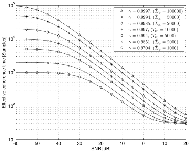
Figure 1: Effective coherence time of the AR1 channel model for various values of the channel forgetting factor.

Figure 1 shows the effective coherence time of the AR1 channel for different values of the channel forgetting factor. In all cases the effective coherence time reaches its limit, ${\hat{T}_{{\rm c}_{0}}}$, at low enough SNR (for ${\hat{T}_{{\rm c}_{0}}}\geq 50,000$ this convergence is not seen in the figure as it happens in lower SNR). For higher SNR the effective coherence time is a decreasing function of the SNR, until it reaches ${\hat{T}_{{\rm c}}}(p_{x})=N$ which is the lowest value measurable in our model.

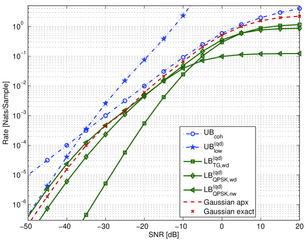
Figure 2: Upper and lower capacity bounds vs. SNR for AR1 fading channel (${\hat{T}_{{\rm c}_{0}}}=900$) and quadratic power constraint ($\alpha=10$).

Figure 2 shows the bounds on the capacity of the AR1 channel with quadratic power constraint when the quadratic constraint constant in (15) is set to $\alpha=10$. The figure shows the capacity bounds when the channel forgetting factor is $\gamma=0.9672$ (${\hat{T}_{{\rm c}_{0}}}=900$). The channel capacity is upper bounded by the low SNR upper bound, ${\rm UB}_{\rm low}^{({\rm qd})}$ (21), which is effective for low SNRs, and by the coherent channel upper bound, ${\rm UB}_{\rm coh}$ (56), which is effective in higher SNRs. In order to demonstrate the role of the different lower bounds we draw 3 lower bound curves. Two of the bounds are based on the QPSK bound (26). For low SNRs the tightest bound uses narrowband QPSK signaling: ${\rm LB_{QPSK,nw}^{(qd)}}=\max_{1\leq\beta\leq\alpha}{\rm LB}_{\rm QPSK}(p_{x},1,\beta)$. For medium SNRs the tightest bound uses wideband QPSK signaling: ${\rm LB_{QPSK,wd}^{(qd)}}=\max_{1\leq\beta\leq\alpha}{\rm LB}_{\rm QPSK}(p_{x},N,\beta)$. For high SNRs the tightest bound uses the truncated Gaussian signaling, (31): ${\rm LB_{TG,wd}^{(qd)}}=\sup_{0<\eta<1}{\rm LB}_{\rm TG}(p_{x},N,1,\eta)$. Note that the upper bounds intersect at $p_{x}=-38.5$ dB. At this point the ratio between the upper bounds and lower bounds is $0.5$. For higher and lower SNR the bounds get tighter, up to the point where, for high enough SNR, the effective coherence time decreases too much and the bounds diverge.

The figure also demonstrates the achievable rates using Gaussian signaling, and the accuracy of the approximation suggested in Section V-A. Using Montecarlo simulations, we evaluated the bound for proper complex Gaussian input distribution (using (84) with $\eta=0$ and the conditional channel covariance matrix from (89)). The resulting rate is depicted in x-marks in Figure 2 (such an evaluation is of course feasible only for short coherence times). The figure also depicts (in a dashed line) the resulting rate when the conditional channel covariance matrix is approximated according to Properties 1–3 in Subsection V-A (which where derived for the case of constant amplitude modulation, and are used here for the approximation of the capacity in the case of Gaussian modulation). As it can be seen, at least for the plotted case, the suggested approximation is very accurate and the approximation error is negligible. The large number of simulations performed have supported this claim, and shown that the approximation accuracy is even better for channels with longer coherence times. Based on these observations we suggest that Gaussian signaling may lead to an even tighter lower bound.

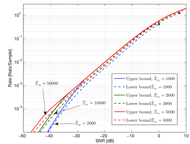
Figure 3: Upper and lower capacity bounds vs. SNR for AR1 fading channel (${\hat{T}_{{\rm c}_{0}}}=2000,10000,50000$) and quadratic power constraint ($\alpha=2$).

Figure 3 depicts the combined capacity bounds for various values of the channel forgetting factor when the quadratic constraint constant is $\alpha=2$. The upper bound (depicted by solid lines) is the bound given by Theorem 1. The lower bound (depicted by dashed lines) is the maximum of the bounds given by Theorems 2 and 3. The figure depicts the bounds for forgetting factors of $\gamma=0.9851,0.997,0.9994$ (which correspond to ${\hat{T}_{{\rm c}_{0}}}=2,000,10,000,$ and $50,000$ respectively).

As it can be seen, the bounds are good in most of the range. The bounds are least tight at SNR values in which the two upper bounds intersect. In these SNR the ratio between the upper and lower bounds is $1.89$, $1.64$ and $1.59$ for ${\hat{T}_{{\rm c}_{0}}}=2,000$, $10,000$ and $50,000$ respectively, very close to the ratio predicted in Section V-B for the case of slowly changing ${\hat{T}_{{\rm c}}}(p_{x})$. For higher and lower SNR the bounds are much tighter. In particular, for high SNR all lower bounds are close to the coherent channel upper bound, but the lower bound is tighter for channels with higher effective coherence time.

The x-marks in the top right end of the lower bounds (for ${\hat{T}_{{\rm c}_{0}}}=2,000$ and ${\hat{T}_{{\rm c}_{0}}}=10,000$) mark the point in which the effective coherence time dropped below ${\hat{T}_{{\rm c}}}(p_{x})=2N=60$. For higher SNR the lower bounds will not be tight. More importantly, for higher SNR our model will not represent well the physical channel, because the assumption that the channel impulse response does not change during one OFDM symbol can no longer be justified. For longer coherence times, this SNR threshold is higher and hence not shown in the figure. For any SNR below the x-marks, the bounds derived in the previous sections are good, and describe the channel capacity with high accuracy.

V-D Comparison to known results

V-D1 Closest results

The bounds which are most similar to the results presented here were derived by Sethuraman et al. [7] and by Durisi et al. [3]. Sethuraman et al. present an upper bound for the frequency-flat fading case ($N=1$) with a peak power constraint. In this case the upper bound in [7] is tighter than the bounds in (22), but the difference is negligible for underspread channels (${\hat{T}_{{\rm c}_{0}}}\gg N$). The difference in the upper bound results from the relaxation $\log(1+x)\leq x$ in (60). This relaxation can be easily avoided, but the resulting bounds are much more complicated for $N>1$, (in particular in the context of underspread channels and effective coherence time) while the difference between the bounds is negligible. Durisi et al. presented upper and lower bounds for frequency selective fading channels, but only for the case of a peak power constraint both in time and in frequency. Both works also presented results on low SNR capacity asymptote that will be discussed in the next subsection.

V-D2 Low SNR limit when ${\hat{T}_{{\rm c}_{0}}}$ exists

In the low SNR limit, if the limit of the effective coherence time, ${\hat{T}_{{\rm c}_{0}}}$, exists as the SNR goes to zero (42), the channel capacity is known and matches the results presented above both with quadratic power constraint and peak power constraint. For the quadratic power constraint [5], the capacity at the low SNR limit is $\alpha{T_{\rm c}}\frac{E[x^{4}]}{2}$, which is exactly equal to the low SNR limit of the upper bound (23). Note that the low SNR limit of the lower bound (30) is lower by a factor of $({\hat{T}_{{\rm c}_{0}}}-N)/{\hat{T}_{{\rm c}_{0}}}$ than the upper bound, which is negligible for ${\hat{T}_{{\rm c}_{0}}}\gg N$. (The main reason for this difference between the upper and lower bounds is the lower bounding transmission scheme which assumes that each OFDM symbol ($N$ samples) is decoded using channel estimation based only on past symbols.)

For the peak power constraint flat fading case ($N=1$), the capacity is $p_{x}^{2}({\hat{T}_{{\rm c}_{0}}}-1)/2$ [7], which matches the results presented here (again up to a negligible factor of $({\hat{T}_{{\rm c}_{0}}}-N)/{\hat{T}_{{\rm c}_{0}}}$ as discussed above). Note that for the peak power constraint we did not analyze the case where the average power constraint is lower than the peak power constraint.

For $N>1$ the same work shows that the low SNR capacity asymptote for the delay separable underspread stationary channel is also given by $p_{x}^{2}({\hat{T}_{{\rm c}_{0}}}-1)/2$. Under the assumption ${\hat{T}_{{\rm c}_{0}}}\gg N$ this channel is approximately equal to the OFDM channel considered here, and the low SNR asymptotes also match. This result also matches the low SNR asymptotes presented in [3] for the case of peak power constraint only in time. It is interesting to note that for this case the peak power constraint used in [7, 3] is stricter than the peak power constraint used here. The power constraint in this work limits the energy of a single OFDM symbol. Translating to the time domain the constraint is applied to the average energy of groups of $N$ samples. On the other hand the constraint in [7] applies for each time domain sample. Interestingly, the bounds are almost identical, even though [7] clearly shows that relaxing the peak power constraint results in a higher capacity for the same average transmission power. Comparing these two works one can conclude that the relaxation of the peak power constraint is effective only if it is applicable for time periods which are at least on the order of the channel coherence time. Allowing signal “peakiness” which must be averaged over periods ($N$) which are significantly shorter than the channel coherence time (${\hat{T}_{{\rm c}_{0}}}$) is not sufficient to increase the channel capacity.

Since the effective coherence time can be interpreted as the block length of a block fading model that achieves the same capacity, our results naturally match results that were derived for the block fading model (e.g., [6, 8]).

V-D3 Analysis for a given channel estimation error

Several works (e.g. [18, 24]) consider the effect of channel estimation error with a given variance on the channel capacity. These works have been the basis for the lower bounds presented here, but they miss the effect of the transmitted signal on the ability to estimate the channel ([18] considers also an estimation from an out-of-band pilot signal). In this sense, one can say that the QPSK lower bound presented above (Theorem 2) is the most straightforward part of the work. It combines an extension of the bounds in [18, 24] to the OFDM model, the channel estimation scheme of [25, 26] which allows to estimate the channel using all (relevant) past transmitted and received symbols, and results on channel estimation errors for constat amplitude modulations. Perhaps the most important contribution of Theorem 2 is the derivation of the bound in a way that shows the role of the effective coherence time. Note that the truncated Gaussian lower bound (Theorem 3) is more complicated as the modulation is not constant amplitude, and the upper bounds are more complicated as they cannot assume any estimation scheme.

V-D4 High SNR limit

As detailed above, for regular channels our analysis holds only up to some finite SNR. The results show that the coherent channel upper bound is achievable as long as the effective coherence time is large enough. This is in agreement with known results [12, 13, 14] showing that in the very high SNR limit the coherent channel upper bound is not achievable. Our analysis cannot predict the actual double logarithmic behavior of the capacity, as it happens at too high SNR where the assumption on the value of the effective coherence time is not valid.

For irregular channels, although not proven, the effective coherence time also typically decreases as SNR increases (although at lower rate). Hence, our analysis is limited in SNR even for irregular channels.

The modeling problem at high SNR is also discussed by Durisi et al. [27], where they focus on the characterization of the range of SNRs in which the channel discretization is reliable. Note that their approach is quite different from the one taken above. In [27], the analysis starts from a continuous time channel, and tries to analyze all modeling errors in the discretization process. In the analysis above we study the behavior of a discrete time OFDM model without assuming any discretization imperfections. Yet, we reach the same conclusion, even the discrete time OFDM model reveals the high SNR model limit.

V-D5 Dependence of coherence time on SNR

Few works analyze the dependence between the SNR and the coherence time. In these works the coherence time characterizes the channel (and does not change for each channel). For example Zheng et al. [28] consider a block-fading channel, where the channel remains constant for a block of $l$ symbols, before changing to an independent realizations. Chen and Veeravalli [29] consider a block stationary channel where the fading is constant across a block of length $T$ and changes in a stationary manner between blocks.

In both cases the analysis considers a set of channels, and tries to characterize relations between the channel coherence time and the system SNR that will result in a certain capacity behavior. Chen and Veeravalli show ([29] equation (21)) that two systems with identical block correlation have the same capacity if the product of their peak powers and block lengths ($T\cdot{\rm SNR}$) is identical.

Zheng et al. analyze the limit capacity of a set of channels with increasing coherence time $l$ and decreasing SNRs. They show that different relations between coherence time and SNR of the form $l={\rm SNR}^{\alpha}$ achieve different capacity behavior between the coherent and noncoherent scheme.

Our analysis is completely different. We consider a (single) specific channel, and show that its effective coherence time is a function of the system SNR.

VI Channel capacity and bounds

In this section we analyze the channel capacity and give the information-theoretical part of the theorem proofs.

In general, even if the input symbols are independent, the output symbols are dependent due to the channel memory. Therefore, we need to evaluate the capacity over the entire transmission, defined as:

$$C=\lim\limits_{n\to\infty}\sup\limits_{{\rm Pr}({\tilde{\bf{X}}_{0}^{n}})}\frac{1}{N(n+1)}I({\tilde{\bf{X}}_{0}^{n}};{\tilde{\bf{Y}}_{0}^{n}}).$$ (53)

Note that the ergodic requirement in Assumption IV guarantees the achievability of the capacity (see for example [12, 6]).

Most of the bounds derived in this section depend on the conditional distribution of the channel given the past transmitted and received symbols. This distribution will be analyzed in detail in the next section. For this section, it is enough to state that given the past symbols, the channel has a complex Gaussian distribution ${\tilde{\bf{H}}_{k}}|{\tilde{\bf{X}}_{0}^{k-1}},{\tilde{\bf{Y}}_{0}^{k-1}}\sim\mathcal{CN}(\tilde{\bm{\mu}}_{k},\tilde{\mathcal{\bm{{\textit{\LARGE$\varepsilon$}}}}}_{k})$. Lemma 3.a also uses the distribution of the channel mean:

$$\tilde{\bm{\mu}}_{k}|{\tilde{\bf{X}}_{0}^{k-1}}\sim\mathcal{CN}\left(E[{\tilde{\bf{H}}_{k}}],{\sf{C}}_{{\tilde{\bf{H}}_{k}}}-\tilde{\mathcal{\bm{{\textit{\LARGE$\varepsilon$}}}}}_{k}\right)$$ (54)

VI-A Coherent channel upper bound

The first upper bound we use is the well known channel capacity when the channel is known to the receiver (coherent channel) with only average power constraint:

$$C \leq \lim\limits_{n\to\infty}\frac{1}{N(n+1)}\sup\limits_{{\rm Pr}({\tilde{\bf{X}}_{0}^{n}})}I({\tilde{\bf{X}}_{0}^{n}};{\tilde{\bf{Y}}_{0}^{n}},{\tilde{\bf{H}}_{0}^{n}})$$ (55)

$$= \lim\limits_{n\to\infty}\frac{1}{N(n+1)}\sum\limits_{k=0}^{n}\sup\limits_{{\rm Pr}({\tilde{\bf{X}}_{k}})}{I({\tilde{\bf{X}}_{k}};{\tilde{\bf{Y}}_{k}},{\tilde{\bf{H}}_{k}})}.$$

$$= \frac{1}{N}\sup\limits_{{\rm Pr}({\tilde{\bf{X}}_{0}})}{I({\tilde{\bf{X}}_{0}};{\tilde{\bf{Y}}_{0}},{\tilde{\bf{H}}_{0}})}.$$

Using Assumptions IV and VI, this bound is maximized when the input signal has Gaussian distribution with $E[{\tilde{\bf{X}}_{k}}]={\rm 0}$, and ${{\rm C}}_{{\tilde{\bf{X}}_{k}}}=p_{x}\cdot{\textsf{I}}$ [30]. The maximal mutual information is given by:

Result 1: The channel capacity is upper bounded by

$$C\leq{\rm UB}_{\rm coh}(p_{x})=E_{{\tilde{\bf{H}}_{0}}}\left[{\log\left(1+Np_{x}|{{\tilde{\bf{h}}_{0,0}}}|^{2}\right)}\right].$$ (56)

The bound in (56) is the capacity of the channel with a constraint only on the average power. As both types of power constraints analyzed here must satisfy $E[{{\bf{p}}_{k}}]\leq Np_{x}$, this bound holds for both types of constraints. As in the case of the block fading model [21], we will show that for large enough effective coherence times and SNR this bound is tight, and the channel capacity does not degrade due to the lack of channel knowledge.

VI-B Low SNR upper bound

The channel capacity is upper bounded by the following lemma:

Lemma 1.a

The capacity of a channel with a peak power constraint is upper bounded by:

$$C \leq \lim\limits_{k\to\infty}\left\{p_{x}\left[1+N\left|E\left[{\tilde{\bf{h}}_{0,0}}\right]\right|^{2}\right]-\frac{1}{N}\log\left(1+N^{2}p_{x}\min_{m}\inf_{{\tilde{\bf{X}}_{0}^{k-1}}\in\mathcal{I}(Np_{x}{\textsf{I}})}(\tilde{\mathcal{\bm{{\textit{\LARGE$\varepsilon$}}}}}_{k})_{m,m}\right)\right\},$$ (57)

and the capacity of a channel with a quadratic power constraint is upper bounded by:

$$C \leq \lim\limits_{k\to\infty}\left\{Np_{x}\left|E\left[{\tilde{\bf{h}}_{0,0}}\right]\right|^{2}\phantom{\sqrt{\sup\limits_{{\rm Pr}({\mathcal{P}}_{k})}E\left[\left\{1-N\min_{m}\inf_{{\tilde{\bf{X}}_{0}^{k-1}}\in\mathcal{I}({\mathcal{P}}_{k-1})}(\tilde{\mathcal{\bm{{\textit{\LARGE$\varepsilon$}}}}}_{k})_{m,m}\right\}^{2}\right]}}\right.$$ (58)

$$+\left.\sqrt{\alpha}p_{x}\sqrt{\sup\limits_{{\rm Pr}({\mathcal{P}}_{k-1})}E\left[\left\{1-N\min_{m}\inf_{{\tilde{\bf{X}}_{0}^{k-1}}\in\mathcal{I}({\mathcal{P}}_{k-1})}(\tilde{\mathcal{\bm{{\textit{\LARGE$\varepsilon$}}}}}_{k})_{m,m}\right\}^{2}\right]}+\frac{1}{2}\alpha Np_{x}^{2}\right\},$$

where $\mathcal{I}({\mathcal{P}}_{k})=\{{\tilde{\bf{X}}_{0}^{k}}:{\tilde{\bf{X}}_{i}^{\dagger}}{\tilde{\bf{X}}_{i}}={{\bf{p}}_{i}},i=0,\ldots,k\}$ is the set of all input symbols that correspond to the power matrix ${\mathcal{P}}_{k}$.

Proof:

We start with the inequality:

$$\lim\limits_{n\to\infty}\frac{1}{N(n+1)}I({\tilde{\bf{X}}_{0}^{n}};{\tilde{\bf{Y}}_{0}^{n}}) = \lim\limits_{n\to\infty}\frac{1}{N(n+1)}\sum\limits_{k=0}^{n}{I({\tilde{\bf{Y}}_{k}};{\tilde{\bf{X}}_{0}^{n}}|{\tilde{\bf{Y}}_{0}^{k-1}})}$$ (59)

$$= \lim\limits_{n\to\infty}\frac{1}{N(n+1)}\sum\limits_{k=0}^{n}\left\{h({\tilde{\bf{Y}}_{k}}|{\tilde{\bf{Y}}_{0}^{k-1}})-h({\tilde{\bf{Y}}_{k}}|{\tilde{\bf{X}}_{0}^{n}},{\tilde{\bf{Y}}_{0}^{k-1}})\right\}$$

$$\leq \lim\limits_{n\to\infty}\frac{1}{N(n+1)}\sum\limits_{k=0}^{n}\left\{h({\tilde{\bf{Y}}_{k}})-h({\tilde{\bf{Y}}_{k}}|{\tilde{\bf{X}}_{0}^{n}},{\tilde{\bf{Y}}_{0}^{k-1}})\right\}.$$

where $h(\cdot)$ is the differential entropy. The first term in the last line of (59) can be upper bounded by the maximal entropy of a random vector with a given covariance matrix. The resulting entropy is [31]:

$$h({\tilde{\bf{Y}}_{k}})\leq\log\left({\|{\sf{C}}_{{\tilde{\bf{Y}}_{k}}}\|}\right)+N\log(\pi e)\leq{\rm Tr}\left(E[{\tilde{\bf{Y}}_{k}}{\tilde{\bf{Y}}_{k}^{\dagger}}]-{{\textsf{I}}}\right)+N\log(\pi e).$$ (60)

where the last inequality uses $\log\left({\left\|{{{\textsf{I}}}+\textsf{A}}\right\|}\right)\leq{\rm Tr}(\textsf{A})$ which holds for any positive semi-definite matrix A. Note that this inequality is tight for low SNR if the transmitted signal has zero mean. Substituting the covariance matrix:

$$E\left[{\tilde{\bf{Y}}_{k}}{\tilde{\bf{Y}}_{k}^{\dagger}}\right]=N\cdot E\left[{\rm diag}({{\tilde{\bf{X}}_{k}}}){{\tilde{\bf{H}}_{k}}}{{\tilde{\bf{H}}_{k}^{\dagger}}}{\rm diag}({{\tilde{\bf{X}}_{k}}})^{\dagger}\right]+{\textsf{I}},$$ (61)

we get:

$$h({\tilde{\bf{Y}}_{k}})-N\log(\pi e) \leq N\cdot{\rm Tr}\left(E\left[{\mathcal{S}}_{{{\bf{X}}_{k}}}\right]\left[{\sf C}_{{\tilde{\bf{H}}_{0}}}+E\left[{\tilde{\bf{H}}_{0}}\right]E\left[{\tilde{\bf{H}}_{0}}\right]^{\dagger}\right]\right)$$ (62)

$$= E\left[{\tilde{\bf{X}}_{k}^{\dagger}}{\tilde{\bf{X}}_{k}}\right]\left[1+N\left|E\left[{\tilde{\bf{h}}_{0,0}}\right]\right|^{2}\right]$$

where the first line uses the rotation property of the trace and the spectrum definition, (2). The second line uses the fact that ${\mathcal{S}}_{{{\bf{X}}_{k}}}$ is a diagonal matrix, while all elements on the diagonal of the second term are equal. We also use the normalization ${\rm Tr}[{\sf{C}}_{{{\bf{H}}_{0}}}]=1$, which results in $({\sf C}_{{\tilde{\bf{H}}_{0}}})_{m,m}=1/N$.

Turning to the second entropy in the last line of (59), we note that the conditional distribution of the output given the input is Gaussian. We also observe that:

$${\sf{C}}_{{\tilde{\bf{Y}}_{k}}|{\tilde{\bf{X}}_{0}^{n}},{\tilde{\bf{Y}}_{0}^{k-1}}}=N\cdot{\rm diag}({{\tilde{\bf{X}}_{k}}})\tilde{\mathcal{\bm{{\textit{\LARGE$\varepsilon$}}}}}_{k}{\rm diag}({{\tilde{\bf{X}}_{k}}})^{\dagger}+{\textsf{I}},$$ (63)

where $\tilde{\mathcal{\bm{{\textit{\LARGE$\varepsilon$}}}}}_{k}$ is the conditional channel covariance matrix given the past transmitted and received symbols. Using (13), the entropy is written as:

$$h({\tilde{\bf{Y}}_{k}}|{\tilde{\bf{X}}_{0}^{n}},{\tilde{\bf{Y}}_{0}^{k-1}})-N\log(\pi e) = E_{{\tilde{\bf{X}}_{0}^{n}},{\tilde{\bf{Y}}_{0}^{k-1}}}\left[{\log\left({\left\|{\sf{C}}_{{\tilde{\bf{Y}}_{k}}|{\tilde{\bf{X}}_{0}^{n}},{\tilde{\bf{Y}}_{0}^{k-1}}}\right\|}\right)}\right]$$ (64)

$$= E_{{\mathcal{P}}_{n}}\left[E_{{\tilde{\bf{X}}_{0}^{n}}|{\mathcal{P}}_{n}}\left[\log\left(\left\|N{\rm diag}({{\tilde{\bf{X}}_{k}}})\tilde{\mathcal{\bm{{\textit{\LARGE$\varepsilon$}}}}}_{k}{\rm diag}({{\tilde{\bf{X}}_{k}}})^{\dagger}+{\textsf{I}}\right\|\right)\right]\right]$$

$$= E_{{\mathcal{P}}_{k}}\left[E_{{\tilde{\bf{X}}_{0}^{k}}|{\mathcal{P}}_{k}}\left[\log\left(\left\|N\tilde{\mathcal{\bm{{\textit{\LARGE$\varepsilon$}}}}}_{k}{\mathcal{S}}_{{{\bf{X}}_{k}}}+{{\textsf{I}}}\right\|\right)\right]\right]$$

$$\geq E_{{\mathcal{P}}_{k}}\left[\inf_{{\tilde{\bf{X}}_{0}^{k}}\in\mathcal{I}({\mathcal{P}}_{k})}\log\left(\left\|N\tilde{\mathcal{\bm{{\textit{\LARGE$\varepsilon$}}}}}_{k}{\mathcal{S}}_{{{\bf{X}}_{k}}}+{{\textsf{I}}}\right\|\right)\right],$$

where we use the rotation property $\left\|{{\textsf{I}}}+\textsf{A}\textsf{B}\right\|=\left\|{{\textsf{I}}}+\textsf{B}\textsf{A}\right\|$.

Now, we observe that since ${\mathcal{S}}_{{{\bf{X}}_{k}}}$ is diagonal and nonnegative,

$${\rm Tr}\left(\tilde{\mathcal{\bm{{\textit{\LARGE$\varepsilon$}}}}}_{k}{\mathcal{S}}_{{{\bf{X}}_{k}}}\right)\geq\min_{m}(\tilde{\mathcal{\bm{{\textit{\LARGE$\varepsilon$}}}}}_{k})_{m,m}{\rm Tr}\left({\mathcal{S}}_{{{\bf{X}}_{k}}}\right).$$ (65)

Using also the inequality $\log\left\|{{\textsf{I}}}+\textsf{A}\right\|\geq\log\left(1+{\rm Tr}(\textsf{A})\right)$ which holds for any positive semi-definite matrix A, the term inside the expectation in the last row of (64) is lower bounded by:

$$\inf_{{\tilde{\bf{X}}_{0}^{k}}\in\mathcal{I}({\mathcal{P}}_{k})}\log\left(\left\|N\tilde{\mathcal{\bm{{\textit{\LARGE$\varepsilon$}}}}}_{k}{\mathcal{S}}_{{{\bf{X}}_{k}}}+{{\textsf{I}}}\right\|\right) \geq \inf_{{\tilde{\bf{X}}_{0}^{k}}\in\mathcal{I}({\mathcal{P}}_{k})}\log\left(1+N{\rm Tr}\left(\tilde{\mathcal{\bm{{\textit{\LARGE$\varepsilon$}}}}}_{k}{\mathcal{S}}_{{{\bf{X}}_{k}}}\right)\right)$$ (66)

$$\geq \log\left(1+N{{\bf{p}}_{k}}\min_{m}\inf_{{\tilde{\bf{X}}_{0}^{k-1}}\in\mathcal{I}({\mathcal{P}}_{k-1})}(\tilde{\mathcal{\bm{{\textit{\LARGE$\varepsilon$}}}}}_{k})_{m,m}\right).$$

Note that this lower bound is achievable using a transmission spectrum that concentrates all of the power on the frequency bin that has minimal estimation error.

Substituting (66) and (62) in (59) results in:

$$C \leq \lim\limits_{n\to\infty}\frac{1}{N(n+1)}\sum\limits_{k=0}^{n}\sup\limits_{{\rm Pr}({\mathcal{P}}_{k})}\Bigg{\{}E\left[{{\bf{p}}_{k}}\right]\left[1+N\left|E\left[{\tilde{\bf{h}}_{0,0}}\right]\right|^{2}\right]$$ (67)

$$-\>E\Big{[}\log\Big{(}1+N{{\bf{p}}_{k}}\min_{m}\inf_{{\tilde{\bf{X}}_{0}^{k-1}}\in\mathcal{I}({\mathcal{P}}_{k-1})}(\tilde{\mathcal{\bm{{\textit{\LARGE$\varepsilon$}}}}}_{k})_{m,m}\Big{)}\Big{]}\Bigg{\}}.$$

Noting also that the resulting quantity is monotonically nondecreasing in $k$, the capacity is upper bounded by:

$$C \leq \frac{1}{N}\lim\limits_{k\to\infty}\sup\limits_{{\rm Pr}({\mathcal{P}}_{k})}\Bigg{\{}E\left[{{\bf{p}}_{k}}\right]\left[1+N\left|E\left[{\tilde{\bf{h}}_{0,0}}\right]\right|^{2}\right]$$ (68)

$$-\>E\Big{[}\log\Big{(}1+N{{\bf{p}}_{k}}\min_{m}\inf_{{\tilde{\bf{X}}_{0}^{k-1}}\in\mathcal{I}({\mathcal{P}}_{k-1})}(\tilde{\mathcal{\bm{{\textit{\LARGE$\varepsilon$}}}}}_{k})_{m,m}\Big{)}\Big{]}\Bigg{\}}.$$

Subject to the peak power constraint, for every $k$ the bound is maximized if ${{\bf{p}}_{k}}=Np_{x}$ (as ${{\bf{p}}_{k}}$ appears inside the log in the second (negative) term). Substituting this optimal transmission power in (68) results in (57) and proves the first part of the lemma.

In order to derive the bound for the quadratic power constraint we use the inequality $\log(1+x)\geq x-\frac{1}{2}x^{2}$ and simplify (68) to:

$$C \leq \frac{1}{N}\lim\limits_{k\to\infty}\sup\limits_{{\rm Pr}({\mathcal{P}}_{k})}\left\{E\left[{{\bf{p}}_{k}}\right]\left[1+N\left|E\left[{\tilde{\bf{h}}_{0,0}}\right]\right|^{2}\right]\phantom{\left[\left\{\inf_{{\tilde{\bf{X}}_{0}^{k-1}}\in\mathcal{I}({\mathcal{P}}_{k-1})}(\tilde{\mathcal{\bm{{\textit{\LARGE$\varepsilon$}}}}}_{k})_{m,m}\right\}^{2}\right]}\right.$$ (69)

$$-\left.E\left[N{{\bf{p}}_{k}}\min_{m}\inf_{{\tilde{\bf{X}}_{0}^{k-1}}\in\mathcal{I}({\mathcal{P}}_{k-1})}(\tilde{\mathcal{\bm{{\textit{\LARGE$\varepsilon$}}}}}_{k})_{m,m}-\frac{1}{2}N^{2}{{\bf{p}}_{k}^{2}}\left\{\min_{m}\inf_{{\tilde{\bf{X}}_{0}^{k-1}}\in\mathcal{I}({\mathcal{P}}_{k-1})}(\tilde{\mathcal{\bm{{\textit{\LARGE$\varepsilon$}}}}}_{k})_{m,m}\right\}^{2}\right]\right\}.$$

Using $(\tilde{\mathcal{\bm{{\textit{\LARGE$\varepsilon$}}}}}_{k})_{m,m}\leq({\sf C}_{{\tilde{\bf{H}}_{0}}})_{m,m}=1/N$, we rewrite (69) as:

$$C \leq \frac{1}{N}\lim\limits_{k\to\infty}\sup\limits_{{\rm Pr}({\mathcal{P}}_{k})}\left\{NE\left[{{\bf{p}}_{k}}\right]\left|E\left[{\tilde{\bf{h}}_{0,0}}\right]\right|^{2}\phantom{\left[\left(\inf_{{\tilde{\bf{X}}_{0}^{k-1}}}(\tilde{\mathcal{\bm{{\textit{\LARGE$\varepsilon$}}}}}_{k})_{m}\right)\right]}\right.$$ (70)

$$+\left.E\left[{{\bf{p}}_{k}}\left(1-N\min_{m}\inf_{{\tilde{\bf{X}}_{0}^{k-1}}\in\mathcal{I}({\mathcal{P}}_{k-1})}(\tilde{\mathcal{\bm{{\textit{\LARGE$\varepsilon$}}}}}_{k})_{m,m}\right)+\frac{1}{2}{{\bf{p}}_{k}^{2}}\right]\right\},$$

and use the Cauchy-Schwartz inequality and the power constraint, (15), to prove (58). ∎

The exact values of the bounds depend on the conditional channel distribution, through $\min_{m}\inf_{{\tilde{\bf{X}}_{0}^{k-1}}\in\mathcal{I}({\mathcal{P}}_{k-1})}(\tilde{\mathcal{\bm{{\textit{\LARGE$\varepsilon$}}}}}_{k})_{m,m}$. This distribution is analyzed in the next section.

VI-C QPSK lower bound

For the lower bound we need to select an input distribution. The first lower bound derived herein is based on QPSK modulation. This bound applies for both power constraints. For the quadratic power constraint, the bound is especially significant at the low SNR regime, where it is crucial to use a low fourth moment. The QPSK modulation uses constant amplitude and hence minimizes the ratio $\frac{E[|{\tilde{\bf{x}}_{k,m}}|^{4}]}{E^{2}[|{\tilde{\bf{x}}_{k,m}}|^{2}]}$.

The input symbol is given by:

$${\tilde{\bf{X}}_{k}}=\sqrt{\beta\frac{N}{r}p_{x}}{\bf g}{\tilde{\bf{B}}_{k}},$$ (71)

where ${\tilde{\bf{B}}_{k}}=\left[{\tilde{\bf{b}}_{k,0}}\ldots,{\tilde{\bf{b}}_{k,r-1}},0,\ldots,0\right]$, $r$ ($1\leq r\leq N$) is the number of active frequency bins, $\{{\tilde{\bf{b}}_{k,m}}\}$ is the sequence of iid QPSK data, and ${\tilde{\bf{b}}_{k,m}}\in\{\pm 1,\pm j\}$ with equal probability. On the other hand, ${\bf g}\in\{0,1\}$ is a binary random variable, statistically independent from ${\tilde{\bf{b}}_{k,0}},\ldots{\tilde{\bf{b}}_{k,r-1}}$, that determines whether the system will transmit or not (i.e., a single variable that affects all transmitted symbols). The transmission probability is ${\rm Pr}({\bf g}=1)=\frac{1}{\beta}$. This distribution is convenient for analysis, although it is not reasonable for practical systems (one cannot consider a practical system that has a positive probability not to transmit any symbol at any time). A practical system can achieve the same performance by transmitting in blocks with large gaps between the blocks, as long as the block length is significantly larger than the channel coherence time.

Lemma 2.a

The capacity of a channel with a quadratic power constraint is lower bounded by:

$$C\geq\lim\limits_{k\to\infty}\max_{r\leq N}\max_{1\leq\beta\leq\alpha}\frac{1}{N\beta}\sum_{m=0}^{r-1}E\left[\left.C_{{\rm QPSK}}\left(\frac{\beta\frac{N^{2}}{r}p_{x}|{\tilde{\bm{\mu}}}_{k,m}|^{2}}{1+\beta\frac{N^{2}}{r}p_{x}(\tilde{\mathcal{\bm{{\textit{\LARGE$\varepsilon$}}}}}_{k})_{m,m}}\right)\right|{\bf g}=1\right],$$ (72)

where $C_{{\rm QPSK}}(\rho)$, defined in (27), is the achievable mutual information for QPSK transmission over AWGN channel with SNR equal to $\rho$ (see for example [20], which also gives some useful bounds). The capacity of a channel with a peak power constraint is lower bounded by:

$$C\geq\lim\limits_{k\to\infty}\max_{r\leq N}\frac{1}{N}\sum_{m=0}^{r-1}E\left[\left.C_{{\rm QPSK}}\left(\frac{\frac{N^{2}}{r}p_{x}|{\tilde{\bm{\mu}}}_{k,m}|^{2}}{1+\frac{N^{2}}{r}p_{x}(\tilde{\mathcal{\bm{{\textit{\LARGE$\varepsilon$}}}}}_{k})_{m,m}}\right)\right|{\bf g}=1\right].$$ (73)

Proof:

As g is constant throughout the transmission, we can safely assume that after long enough time the receiver can decode ${\bf g}$ with no error. Thus, we can write:

$$\lim\limits_{n\to\infty}\frac{1}{N(n+1)}I({\tilde{\bf{X}}_{0}^{n}};{\tilde{\bf{Y}}_{0}^{n}}) = \lim\limits_{n\to\infty}\frac{1}{N(n+1)}I({\tilde{\bf{X}}_{0}^{n}};{\tilde{\bf{Y}}_{0}^{n}}|{\bf g})$$ (74)

$$= \frac{1}{\beta}\lim\limits_{n\to\infty}\frac{1}{N(n+1)}I({\tilde{\bf{B}}_{0}^{n}};{\tilde{\bf{Y}}_{0}^{n}}|{\bf g}=1).$$

Given ${\bf g}=1$ the transmitted symbols are statistically independent. We use the following equality:

$$I({\tilde{\bf{B}}_{0}^{n}};{\tilde{\bf{Y}}_{0}^{n}}|{\bf g}=1) = \sum\limits_{k=0}^{n}{I({\tilde{\bf{B}}_{k}};{\tilde{\bf{Y}}_{k}}|{\bf g}=1,{\tilde{\bf{B}}_{0}^{k-1}},{\tilde{\bf{Y}}_{0}^{k-1}},{\tilde{\bf{Y}}_{k+1}^{n}})}$$ (75)

$$+\sum\limits_{k=0}^{n}{I({\tilde{\bf{B}}_{k}};{\tilde{\bf{Y}}_{0}^{k-1}}|{\bf g}=1,{\tilde{\bf{B}}_{0}^{k-1}},{\tilde{\bf{Y}}_{k+1}^{n}})}$$

$$+\sum\limits_{k=0}^{n}{I({\tilde{\bf{B}}_{k}};{\tilde{\bf{Y}}_{k+1}^{n}}|{\bf g}=1,{\tilde{\bf{B}}_{0}^{k-1}})}$$

The second and third terms on the right hand side of this equation correspond to the mutual information between an input symbol and the past or future output symbols. As these terms do not use the $k$-th symbol output, they both vanish when the input symbols are iid. The first term can be lower bounded by:

$$I({\tilde{\bf{B}}_{0}^{n}};{\tilde{\bf{Y}}_{0}^{n}}|{\bf g}=1) = \sum\limits_{k=0}^{n}{I({\tilde{\bf{B}}_{k}};{\tilde{\bf{Y}}_{k}}|{\bf g}=1,{\tilde{\bf{B}}_{0}^{k-1}},{\tilde{\bf{Y}}_{0}^{k-1}},{\tilde{\bf{Y}}_{k+1}^{n}})}$$ (76)

$$\geq \sum\limits_{k=0}^{n}{I({\tilde{\bf{B}}_{k}};{\tilde{\bf{Y}}_{k}}|{\bf g}=1,{\tilde{\bf{B}}_{0}^{k-1}},{\tilde{\bf{Y}}_{0}^{k-1}})}$$

$$\geq \sum\limits_{k=0}^{n}\sum\limits_{m=0}^{r-1}{I({\tilde{\bf{b}}_{k,m}};{\tilde{\bf{y}}_{k,m}}|{\bf g}=1,{\tilde{\bf{B}}_{0}^{k-1}},{\tilde{\bf{Y}}_{0}^{k-1}})},$$

where the second line uses the statistical independence of ${\tilde{\bf{Y}}_{k+1}^{n}}$ and ${\tilde{\bf{B}}_{k}}$, and the third line uses the statistical independence between the elements of ${\tilde{\bf{B}}_{k}}$. Substituting (76) in (74), and noting again that the term inside the summation is monotonic in $k$, results in the lower bound on the capacity:

$$C\geq\lim\limits_{k\to\infty}\frac{1}{N\beta}\sum\limits_{m=0}^{r-1}{I({\tilde{\bf{b}}_{k,m}};{\tilde{\bf{y}}_{k,m}}|{\tilde{\bf{B}}_{0}^{k-1}},{\tilde{\bf{Y}}_{0}^{k-1}},{\bf g}=1)}.$$ (77)

Note that the past symbols affect the distribution of the current symbol only through the conditional distribution of the channel. Thus, in this lower bound, the decoding of correlated output symbols is replaced by the decoding of uncorrelated symbols with channel state information (CSI). This CSI is produced by optimal channel estimation based on past input and output symbols. A coding scheme that allows to decode the previous symbols and use them for channel estimation for the next symbol is shown in [25, 26].

Focusing on the $m$-th frequency bin of the $k$-th symbol, given ${\bf g}=1$, the channel output is:

$${\tilde{\bf{y}}_{k,m}}=\sqrt{\frac{\beta}{r}p_{x}}N{\tilde{\bm{\mu}}}_{k,m}{\tilde{\bf{b}}_{k,m}}+{\tilde{\bf{w}}_{k,m}}+{\tilde{\bf{v}}_{k,m}}.$$ (78)

where ${\tilde{\bf{w}}_{k,m}}$ is the $m$-th element of the DFT of the Complex Gaussian noise, and ${\tilde{\bf{v}}_{k,m}}=\sqrt{\frac{\beta}{r}p_{x}}N({\tilde{\bf{h}}_{k,m}}-{\tilde{\bm{\mu}}}_{k,m}){\tilde{\bf{b}}_{k,m}}$ is the interference term due to channel estimation error. Since the estimation error is a circularly symmetric Gaussian random variable and the data has constant amplitude, the interference term is also Gaussian and is statistically independent from the data (${\tilde{\bf{b}}_{k,m}}$). Assuming optimal channel estimation, the resulting channel is equivalent to a coherent flat fading channel with additive independent complex Gaussian noise samples of variance $1+\beta\frac{N^{2}}{r}p_{x}(\tilde{\mathcal{\bm{{\textit{\LARGE$\varepsilon$}}}}}_{k})_{m,m}$. Evaluating the mutual information of this channel for QPSK modulation and multiplying it by the transmission probability ($1/\beta$) leads to (72) and (73), depending on the allowed range of the parameter $\beta$. ∎

VI-D Truncated Gaussian lower bound

For high SNR, the QPSK bound will not be tight (most obviously as it is limited to 2 bits per frequency bin). The most intuitive alternative is a complex Gaussian input distribution. Such a distribution seems very close to optimal (based on a large set of simulations). However, we were unable to produce an appropriate bound on the resulting conditional channel variance, and therefore turned to a slightly modified distribution.

Let ${\bf u}$ be a proper complex Gaussian distribution, ${\bf u}\sim\mathcal{CN}(0,1)$. We denote hereafter by truncated Gaussian distribution with parameters $\eta$ and $\xi$ the distribution of ${\bf u}$ given : $\eta\leq|{\bf u}|^{2}\leq\xi$. In mathematical terms, we say that ${\bf z}\sim\mathcal{TCN}(\eta,\xi)$ if for any function $f(\cdot)$ we have:

$$E\left[f({\bf z})\right]=E\left[f({\bf u})\Big{|}\eta\leq|{\bf u}|^{2}\leq\xi\right].$$ (79)

Note that $|{\bf u}|^{2}$ has an exponential distribution with parameter 1. Define:

$$\theta=\textrm{Pr}({{\eta\leq|{\bf u}|^{2}\leq\xi}})=e^{-\eta}-e^{-\xi}.$$ (80)

The second moment of the truncated Gaussian distribution is:

$$p_{z} = \frac{1}{\theta}\int_{\eta}^{\xi}{\chi e^{-\chi}d\chi}=1+\frac{\eta e^{-\eta}-\xi e^{-\xi}}{e^{-\eta}-e^{-\xi}}.$$ (81)

The Fourth moment of the truncated Gaussian distribution is:

$$E\left[|{\bf z}|^{4}\right] = \frac{1}{\theta}\int_{\eta}^{\xi}{\chi^{2}e^{-\chi}d\chi}=2+\frac{(\eta^{2}+2\eta)e^{-\eta}-(\xi^{2}+2\xi)e^{-\xi}}{e^{-\eta}-e^{-\xi}}$$ (82)

Using the truncated Gaussian distribution, we define the input symbol as:

$${\tilde{\bf{X}}_{k}}=\frac{c}{\sqrt{p_{z}}}{\bf g}{\tilde{\bf{Z}}_{k}},$$ (83)

where $c$ is chosen to satisfy the power constraint, $\bf g$ is defined as in the QPSK lower bound, ${\tilde{\bf{Z}}_{k}}=\left[{\tilde{\bf{z}}_{k,0}}\ldots,{\tilde{\bf{z}}_{k,r-1}},0,\ldots,0\right]$, $1\leq r\leq N$ is the number of active frequency bins, and $\{{\tilde{\bf{z}}_{k,m}}\}$ is the sequence of iid input random variables with truncated Gaussian distribution ${\tilde{\bf{z}}_{k,m}}\sim\mathcal{TCN}(\eta,\xi)$.

Lemma 3.a

If $E[{\tilde{\bf{h}}_{0,m}}]=0$, the capacity of a channel with a quadratic power constraint (and $\alpha>1$) is lower bounded by:

$$C \geq \lim\limits_{k\to\infty}\max_{r\leq N}\sup_{\eta>0}\max_{1\leq\beta\leq\frac{\alpha r(1+\eta)^{2}}{1+r(1+\eta)^{2}}}-\frac{r\eta}{N\beta}$$ (84)

$$+\frac{1}{N\beta}\sum_{m=0}^{r-1}\log\left(1+\frac{\beta\frac{N^{2}}{r}p_{x}\left(\frac{1}{N}-E\left[\left.(\tilde{\mathcal{\bm{{\textit{\LARGE$\varepsilon$}}}}}_{k})_{m,m}\right|{\bf g}=1\right]\right)\left|{\bf u}\right|^{2}}{1+\beta\frac{N^{2}}{r}p_{x}E\left[\left.(\tilde{\mathcal{\bm{{\textit{\LARGE$\varepsilon$}}}}}_{k})_{m,m}\right|{\bf g}=1\right]}\right)$$

and the capacity of a channel with a peak power constraint is lower bounded by:

$$C \geq \lim\limits_{k\to\infty}\max_{r\leq N}\sup_{0<\eta<\xi}\frac{1}{N}\sum_{m=0}^{r-1}\log\left(1+\frac{\frac{N^{2}p_{x}p_{z}}{r\xi}\left(\frac{1}{N}-E\left[\left.(\tilde{\mathcal{\bm{{\textit{\LARGE$\varepsilon$}}}}}_{k})_{m,m}\right|{\bf g}=1\right]\right)\left|{\bf u}\right|^{2}}{1+\frac{N^{2}p_{x}p_{z}}{r\xi}E\left[\left.(\tilde{\mathcal{\bm{{\textit{\LARGE$\varepsilon$}}}}}_{k})_{m,m}\right|{\bf g}=1\right]}\right)$$ (85)

$$+\frac{r}{N\beta}\log(e^{-\eta}-e^{-\xi}).$$

where ${\bf u}$ is a proper complex Gaussian random variable $\left({\bf u}\sim\mathcal{CN}(0,1)\right)$ and $\eta$ and $\xi$ are the thresholds used to define the truncated Gaussian distribution.

As in the previous bounds, this lower bound depends on the conditional channel distribution (through the expectation of the conditional channel covariance matrix). Note that the covariance matrix itself also depends on the definition of the truncated Gaussian distribution, i.e., on the parameters $\eta$ and $\xi$.

Proof of Lemma 3.a: See Appendix A.

VII Channel estimation

In this section we analyze the conditional distribution of the channel given the past transmitted and received symbols, and provide the bounds required for the capacity evaluation.

Using Assumption III (no feedback) the transmitted signal is statistically independent from the channel, and hence, given the input symbols ${\tilde{\bf{X}}_{0}^{k-1}}$, the output symbols ${\tilde{\bf{Y}}_{0}^{k-1}}$ are jointly Gaussian with the channel ${\tilde{\bf{H}}_{0}^{k}}$. Thus, the desired distribution can be analyzed through the theory of optimal linear estimation. The auto-covariance of the conditioned output symbols, ${\tilde{\bf{Y}}_{0}^{k-1}}|{\tilde{\bf{X}}_{0}^{k-1}}$, is:

$${{\rm C}}_{{\tilde{\bf{Y}}_{0}^{k-1}}|{\tilde{\bf{X}}_{0}^{k-1}}}=N{\rm diag}({\tilde{\bf{X}}_{0}^{k-1}}){\sf{C}}_{{\tilde{\bf{H}}_{0}^{k-1}}}{\rm diag}({\tilde{\bf{X}}_{0}^{k-1}})^{\dagger}+{\textsf{I}}$$ (86)

and their cross covariance matrix with ${\tilde{\bf{H}}_{k}}$ is:

$${{\rm C}}_{{\tilde{\bf{Y}}_{0}^{k-1}},{\tilde{\bf{H}}_{k}}|{\tilde{\bf{X}}_{0}^{k-1}}}=\sqrt{N}\cdot{\rm diag}({\tilde{\bf{X}}_{0}^{k-1}}){\sf{C}}_{{\tilde{\bf{H}}_{0}^{k-1}},{\tilde{\bf{H}}_{k}}}$$ (87)

where ${\sf{C}}_{{\tilde{\bf{H}}_{0}^{k-1}},{\tilde{\bf{H}}_{k}}}$ is the sub-matrix of ${\sf{C}}_{{\tilde{\bf{H}}_{0}^{k-1}}}$ describing the cross covariance between current channel vector and the past channel vectors. Therefore, ${\tilde{\bf{H}}_{k}}|{\tilde{\bf{X}}_{0}^{k-1}},{\tilde{\bf{Y}}_{0}^{k-1}}$ has complex Gaussian distribution ${\tilde{\bf{H}}_{k}}|{\tilde{\bf{X}}_{0}^{k-1}},{\tilde{\bf{Y}}_{0}^{k-1}}\sim\mathcal{CN}(\tilde{\bm{\mu}}_{k},\tilde{\mathcal{\bm{{\textit{\LARGE$\varepsilon$}}}}}_{k})$, where the conditional channel mean, $\tilde{\bm{\mu}}_{k}$, and the conditional channel covariance matrix, $\tilde{\mathcal{\bm{{\textit{\LARGE$\varepsilon$}}}}}_{k}$, are given by [32]:

$$\tilde{\bm{\mu}}_{k} = E[{\tilde{\bf{H}}_{k}}]+\sqrt{N}{{\sf{C}}_{{\tilde{\bf{H}}_{0}^{k-1}},{\tilde{\bf{H}}_{k}}}^{\dagger}}{\rm diag}({\tilde{\bf{X}}_{0}^{k-1}})^{\dagger}\left(N{\rm diag}({\tilde{\bf{X}}_{0}^{k-1}}){\sf{C}}_{{\tilde{\bf{H}}_{0}^{k-1}}}{\rm diag}({\tilde{\bf{X}}_{0}^{k-1}})^{\dagger}+{\textsf{I}}\right)^{-1}$$ (88)

$$\cdot\left({\tilde{\bf{Y}}_{0}^{k-1}}-\sqrt{N}{\rm diag}({\tilde{\bf{X}}_{0}^{k-1}})E[{\tilde{\bf{H}}_{0}^{k-1}}]\right)$$

$$\tilde{\mathcal{\bm{{\textit{\LARGE$\varepsilon$}}}}}_{k} = {\sf{C}}_{{\tilde{\bf{H}}_{k}}}-N{{\sf{C}}_{{\tilde{\bf{H}}_{0}^{k-1}},{\tilde{\bf{H}}_{k}}}^{\dagger}}{\rm diag}({\tilde{\bf{X}}_{0}^{k-1}})^{\dagger}\left(N{\rm diag}({\tilde{\bf{X}}_{0}^{k-1}}){\sf{C}}_{{\tilde{\bf{H}}_{0}^{k-1}}}{\rm diag}({\tilde{\bf{X}}_{0}^{k-1}})^{\dagger}+{\textsf{I}}\right)^{-1}$$ (89)

$$\cdot{\rm diag}({\tilde{\bf{X}}_{0}^{k-1}}){{\sf{C}}_{{\tilde{\bf{H}}_{0}^{k-1}},{\tilde{\bf{H}}_{k}}}}.$$

We note that the conditional channel mean is characterized by the conditional channel covariance matrix, $\tilde{\mathcal{\bm{{\textit{\LARGE$\varepsilon$}}}}}_{k}$, since we can write the distribution of the channel mean as $\tilde{\bm{\mu}}_{k}|{\tilde{\bf{X}}_{0}^{k-1}}\sim\mathcal{CN}\left(E[{\tilde{\bf{H}}_{k}}],{\sf{C}}_{{\tilde{\bf{H}}_{k}}}-\tilde{\mathcal{\bm{{\textit{\LARGE$\varepsilon$}}}}}_{k}\right)$. Therefore, we will focus hereon on the characterization of the conditional channel covariance matrix $\tilde{\mathcal{\bm{{\textit{\LARGE$\varepsilon$}}}}}_{k}$.

In this section we characterize the bounds on $(\tilde{\mathcal{\bm{{\textit{\LARGE$\varepsilon$}}}}}_{k})_{m,m}$ and its moments in terms of the effective coherence time.

Lemma 1.b

With a peak power constraint, the conditional channel covariance matrix is lower bounded by:

$$\lim\limits_{k\to\infty}\min_{m}\inf_{{\tilde{\bf{X}}_{0}^{k-1}}\in\mathcal{I}(Np_{x}{\textsf{I}})}(\tilde{\mathcal{\bm{{\textit{\LARGE$\varepsilon$}}}}}_{k})_{m,m} \geq \frac{1}{N}\frac{1}{1+\frac{p_{x}}{2}({\hat{T}_{{\rm c}}}(p_{x})-N)}.$$ (90)

With a quadratic power constraint, the conditional channel covariance matrix satisfies:

$$\lim\limits_{k\to\infty}\sup\limits_{{\rm Pr}({\mathcal{P}}_{k-1})}E\left[\left\{1-N\min_{m}\inf_{{\tilde{\bf{X}}_{0}^{k-1}}\in\mathcal{I}({\mathcal{P}}_{k-1})}(\tilde{\mathcal{\bm{{\textit{\LARGE$\varepsilon$}}}}}_{k})_{m,m}\right\}^{2}\right] \leq \alpha\left(1-\frac{1}{1+\frac{p_{x}}{2}({\hat{T}_{{\rm c}}}(p_{x})-N)}\right)^{2},$$ (91)

Proof:

In Appendix B we prove the following inequality:

$$(\tilde{\mathcal{\bm{{\textit{\LARGE$\varepsilon$}}}}}_{k})_{m,m} \geq \frac{1}{N}\left[1-{{D}_{k}^{\dagger}}{\mathcal{P}}_{k-1}\left({\textsf{I}}+{{{\Delta}_{k-1}}}{\mathcal{P}}_{k-1}\right)^{-1}{{D}_{k}}\right].$$ (92)

The proof is based on showing that the conditional covariance is minimized using ${\mathcal{S}}_{{{\bf{X}}_{0}^{k-1}}}={\mathcal{P}}_{k-1}\otimes{\textsf{J}}_{m}$, where ${\textsf{J}}_{m}$ is an $N\times N$ matrix with only one nonzero element, the $m$-th element on the diagonal, which equals 1.

The first part of the lemma follows directly from (92) by noting that the conditional covariance matrix is a nonincreasing function of each element in ${\mathcal{P}}_{k-1}$. Therefore, it is minimized when all elements take their maximal value (${\mathcal{P}}_{k-1}=Np_{x}{\textsf{I}}$), so that

$$\lim\limits_{k\to\infty}\min_{m}\inf_{{\tilde{\bf{X}}_{0}^{k-1}}\in\mathcal{I}(Np_{x}{\textsf{I}})}(\tilde{\mathcal{\bm{{\textit{\LARGE$\varepsilon$}}}}}_{k})_{m,m} \geq \frac{1}{N}\left[1-\lim\limits_{k\to\infty}Np_{x}{{D}_{k}^{\dagger}}\left({\textsf{I}}+Np_{x}{{{\Delta}_{k-1}}}\right)^{-1}{{D}_{k}}\right].$$ (93)

Using the definition of the effective coherence time, (16), and the matrix inversion lemma leads to (90) and completes the first part of the proof.

For the quadratic case the bounding is slightly more complicated, and we search for bounds on moments of the conditional covariance matrix that will hold for any distribution of the transmission powers, ${\mathcal{P}}_{k-1}$. To do so, we use the same derivation as in (B.4), and apply it to (92) with ${\mathcal{P}}_{k-1}=E[{\mathcal{P}}_{k-1}]+\breve{\mathcal{P}}$. We get:

$$(\tilde{\mathcal{\bm{{\textit{\LARGE$\varepsilon$}}}}}_{k})_{m,m} \geq \frac{1}{N}-\frac{1}{N}{{D}_{k}^{\dagger}}E[{\mathcal{P}}_{k-1}]\left({\textsf{I}}+{{{\Delta}_{k-1}}}{E[{\mathcal{P}}_{k-1}]}\right)^{-1}{{D}_{k}}$$ (94)

$$-\frac{1}{N}{{D}_{k}^{\dagger}}\left({\textsf{I}}+{E[{\mathcal{P}}_{k-1}]}{{{\Delta}_{k-1}}}\right)^{-1}\breve{\mathcal{P}}\left({\textsf{I}}+{{{\Delta}_{k-1}}}{E[{\mathcal{P}}_{k-1}]}\right)^{-1}{{D}_{k}}.$$

Taking the expectation of the square of (94) and using $(\tilde{\mathcal{\bm{{\textit{\LARGE$\varepsilon$}}}}}_{k})_{m,m}\leq\frac{1}{N}$, we have:

$$E\left[\left\{1-N(\tilde{\mathcal{\bm{{\textit{\LARGE$\varepsilon$}}}}}_{k})_{m,m}\right\}^{2}\right] \leq \left({{D}_{k}^{\dagger}}E[{\mathcal{P}}_{k-1}]\left({\textsf{I}}+{{{\Delta}_{k-1}}}E[{\mathcal{P}}_{k-1}]\right)^{-1}{{D}_{k}}\right)^{2}+E\left[{V^{\dagger}\breve{\mathcal{P}}VV^{\dagger}\breve{\mathcal{P}}V}\right].$$ (95)

where ${{V}}=\left({\textsf{I}}+{{{\Delta}_{k-1}}}E[{\mathcal{P}}_{k-1}]\right)^{-1}{{D}_{k}}$. Focusing on the second term in the righthand side of (95) we have:

$$E\left[{V^{\dagger}\breve{\mathcal{P}}VV^{\dagger}\breve{\mathcal{P}}V}\right] = E\left[\sum_{a}\sum_{b}v^{*}_{a}\breve{\mathcal{P}}_{a,a}v_{a}v^{*}_{b}\breve{\mathcal{P}}_{b,b}v_{b}\right]$$ (96)

$$= \sum_{a}\sum_{b}\left|v_{a}\right|^{2}\left|v_{b}\right|^{2}E\left[\breve{\mathcal{P}}_{a,a}\breve{\mathcal{P}}_{b,b}\right]$$

$$\leq \sum_{a}\sum_{b}\left|v_{a}\right|^{2}\left|v_{b}\right|^{2}\sqrt{E\left[\breve{\mathcal{P}}_{a,a}^{2}\right]E\left[\breve{\mathcal{P}}_{b,b}^{2}\right]}$$

$$\leq (\alpha-1)N^{2}p_{x}^{2}(V^{\dagger}V)^{2}$$

where we use $\breve{\mathcal{P}}_{b,b}={{\bf{p}}_{b}}-E[{{\bf{p}}_{b}}]$, and hence $E\left[\breve{\mathcal{P}}_{b,b}^{2}\right]\leq(\alpha-1)N^{2}p_{x}^{2}$. Substituting back in (95), we observe that the righthand side of (95) is maximized with $E[{\mathcal{P}}_{k-1}]=Np_{x}{\textsf{I}}$ and we get:

$$E\left[\left\{1-N(\tilde{\mathcal{\bm{{\textit{\LARGE$\varepsilon$}}}}}_{k})_{m,m}\right\}^{2}\right] \leq N^{2}p_{x}^{2}\left({{D}_{k}^{\dagger}}\left({\textsf{I}}+Np_{x}{{{\Delta}_{k-1}}}\right)^{-1}{{D}_{k}}\right)^{2}$$ (97)

$$+\>(\alpha-1)N^{2}p_{x}^{2}\left({{D}_{k}^{\dagger}}\left({\textsf{I}}+Np_{x}{{{\Delta}_{k-1}}}\right)^{-2}{{D}_{k}}\right)^{2}$$

$$\leq N^{2}p_{x}^{2}\left({{D}_{k}^{\dagger}}\left({\textsf{I}}+Np_{x}{{{\Delta}_{k-1}}}\right)^{-1}{{D}_{k}}\right)^{2}$$

$$+\>(\alpha-1)N^{2}p_{x}^{2}\left({{D}_{k}^{\dagger}}\left({\textsf{I}}+Np_{x}{{{\Delta}_{k-1}}}\right)^{-1}{{D}_{k}}\right)^{2}$$

$$= \alpha N^{2}p_{x}^{2}\left({{D}_{k}^{\dagger}}\left({\textsf{I}}+Np_{x}{{{\Delta}_{k-1}}}\right)^{-1}{{D}_{k}}\right)^{2}$$

where the second inequality in (97) uses the fact that all eigenvalues of ${\textsf{I}}+Np_{x}{{{\Delta}_{k-1}}}$ are larger or equal to 1, and therefore $\left({\textsf{I}}+Np_{x}{{{\Delta}_{k-1}}}\right)^{-1}\geq\left({\textsf{I}}+Np_{x}{{{\Delta}_{k-1}}}\right)^{-2}$. Using the effective coherence time definition results in (91) and completes the proof of the lemma. ∎

Lemma 2.b

Using QPSK modulation, as defined in (71), for each active frequency bin ($0\leq m\leq r-1$) the diagonal element of the conditional channel covariance matrix is lower bounded by:

$$\lim\limits_{k\to\infty}(\tilde{\mathcal{\bm{{\textit{\LARGE$\varepsilon$}}}}}_{k})_{m,m} \leq \left\{\begin{array}[]{ll}\frac{1}{N}\frac{1}{1+\frac{\beta}{L}\frac{p_{x}}{2}\left({\hat{T}_{{\rm c}}}\left(\beta p_{x}\right)-N\right)}&r=N\\ \frac{1}{N}\frac{1}{1+\frac{\beta}{r}\frac{p_{x}}{2}\left({\hat{T}_{{\rm c}}}\left(\frac{\beta}{r}p_{x}\right)-N\right)}&r<N\end{array}\right.$$ (100)

Proof:

Starting with the wideband QPSK modulation ($r=N$), the transmission spectrum given $\textbf{g}=1$ is equal to ${\mathcal{S}}_{{{\bf{X}}_{0}^{k-1}}}=\beta p_{x}{\textsf{I}}$. Substituting in the estimation error covariance matrix, (89) (see also (B.3)), we have:

$$\tilde{{\bm{{\textit{\LARGE$\varepsilon$}}}}}_{k}={\sf{C}}_{{\tilde{\bf{H}}_{k}}}-N\beta p_{x}{{\sf{C}}_{{\tilde{\bf{H}}_{0}^{k-1}},{\tilde{\bf{H}}_{k}}}^{\dagger}}\left(N\beta p_{x}{\sf{C}}_{{\tilde{\bf{H}}_{0}^{k-1}}}+{\textsf{I}}\right)^{-1}{{\sf{C}}_{{\tilde{\bf{H}}_{0}^{k-1}},{\tilde{\bf{H}}_{k}}}}.$$ (101)

Writing the estimation error covariance matrix, (101), in the time domain, and substituting (11) we have:

$${\bm{{\textit{\LARGE$\varepsilon$}}}}_{k}={\sf{F}}\tilde{{\bm{{\textit{\LARGE$\varepsilon$}}}}}_{k}{\sf{F}}^{\dagger}={\sf{C}}_{{{\bf{H}}_{k}}}-N\beta p_{x}{{D}_{k}^{\dagger}}\otimes{\sf{C}}_{{{\bf{H}}_{k}}}\left(N\beta p_{x}{{\Delta}_{k-1}}\otimes{\sf{C}}_{{{\bf{H}}_{k}}}+{\textsf{I}}\right)^{-1}{{D}_{k}}\otimes{\sf{C}}_{{{\bf{H}}_{k}}}.$$ (102)

Note that covariance matrices are hermitian so that ${\sf{C}}_{{{\bf{H}}_{k}}}^{\dagger}={\sf{C}}_{{{\bf{H}}_{k}}}$. In Appendix C we show that this is a diagonal matrix in which the $l$-th element on the diagonal is given by:

$$({\bm{{\textit{\LARGE$\varepsilon$}}}}_{k})_{l,l} = ({\sf{C}}_{{{\bf{H}}_{k}}})_{l,l}-N\beta p_{x}{{D}_{k}^{\dagger}}({\sf{C}}_{{{\bf{H}}_{k}}})_{l,l}\left(N\beta p_{x}{{\Delta}_{k-1}}({\sf{C}}_{{{\bf{H}}_{k}}})_{l,l}+{\textsf{I}}\right)^{-1}{{D}_{k}}({\sf{C}}_{{{\bf{H}}_{k}}})_{l,l}.$$ (103)

For any channel tap such that $({\sf{C}}_{{{\bf{H}}_{k}}})_{l,l}>0$ we can use the matrix inversion lemma to write the inverse of the estimation error as:

$$({{\bm{{\textit{\LARGE$\varepsilon$}}}}}_{k})_{l,l}^{-1} = ({\sf{C}}_{{{\bf{H}}_{k}}})_{l,l}^{-1}+N\beta p_{x}{{D}_{k}^{\dagger}}\cdot\left(N\beta p_{x}({\sf{C}}_{{{\bf{H}}_{k}}})_{l,l}\left[{{\Delta}_{k-1}}-{{D}_{k}}{{D}_{k}^{\dagger}}\right]+{\textsf{I}}\right)^{-1}{{D}_{k}}$$ (104)

and taking the limit as $k$ goes to infinity:

$$\lim\limits_{k\to\infty}({{\bm{{\textit{\LARGE$\varepsilon$}}}}}_{k})_{l,l}^{-1} = ({\sf{C}}_{{{\bf{H}}_{k}}})_{l,l}^{-1}+\frac{\beta p_{x}}{2}\left({\hat{T}_{{\rm c}}}\left(\beta p_{x}({\sf{C}}_{{{\bf{H}}_{k}}})_{l,l}\right)-N\right)$$ (105)

$$\geq ({\sf{C}}_{{{\bf{H}}_{k}}})_{l,l}^{-1}+\frac{\beta p_{x}}{2}({\hat{T}_{{\rm c}}}\left(\beta p_{x}\right)-N).$$

Going back to the frequency domain, the properties of the DFT guarantee that all elements on the diagonal of $\tilde{\bm{{\textit{\LARGE$\varepsilon$}}}}_{k}$ are equal. We therefore have:

$$\lim\limits_{k\to\infty}(\tilde{\mathcal{\bm{{\textit{\LARGE$\varepsilon$}}}}}_{k})_{m,m} = \frac{1}{N}{\rm Tr}\left\{\lim\limits_{k\to\infty}{\bm{{\textit{\LARGE$\varepsilon$}}}}_{k}\right\}\leq\frac{1}{N}\sum_{l:({\rm C}_{{{\bf{H}}_{k}}})_{l,l}\neq 0}\frac{1}{({\rm C}_{{{\bf{H}}_{k}}})_{l,l}^{-1}+\beta\frac{p_{x}}{2}\left({\hat{T}_{{\rm c}}}\left(\beta p_{x}\right)-N\right)}.$$ (106)

Using the concavity of the function $(a+1/x)^{-1}$ for positive $a$ and ${\rm Tr}[{\sf{C}}_{{{\bf{H}}_{k}}}]=1$ proves the first (upper) part of (100).

For $r<N$ we lower bound the diagonal element of the conditional channel covariance matrix by the performance of a sub-optimal estimation scheme. This estimation scheme estimates the channel at the $m$-th frequency bin based only on data transmitted and received over the $m$ frequency bin. Inspecting (101) and taking only the elements that correspond to the $m$ frequency bin ($0\leq m\leq r-1$) the conditional channel variance is lower bounded by:

$$(\tilde{\bm{{\textit{\LARGE$\varepsilon$}}}}_{k})_{m,m}\leq\frac{1}{N}-\frac{1}{N}\beta\frac{N}{r}p_{x}D_{k}^{\dagger}\left(\beta\frac{N}{r}p_{x}\Delta_{k-1}+{\textsf{I}}\right)^{-1}D_{k}.$$ (107)

where we took into account the normalization $({\sf{C}}_{{\tilde{\bf{H}}_{k}}})_{m,m}=\frac{1}{N}$ and the fact that the transmitted power for an active bin, given $\textbf{g}=1$, is $\beta\frac{N}{r}p_{x}$. Using the matrix inversion lemma and the definition of the effective coherence time, (16), results in the second part of (100) and completes the proof of the lemma. ∎

Lemma 3.b

Using truncated Gaussian input distribution, as defined in (83), for each active frequency bin ($0\leq m\leq r-1$) the mean of the diagonal element of the conditional channel covariance matrix is lower bounded for quadratic power constraint by:

$$\lim\limits_{k\to\infty}E\left[(\tilde{\mathcal{\bm{{\textit{\LARGE$\varepsilon$}}}}}_{k})_{m,m}\right] \leq \left\{\begin{array}[]{ll}\frac{1}{N}\frac{1}{1+\frac{\beta p_{x}}{(1+\eta)\log(1+\frac{1}{\eta})}\frac{1}{2L}\left({\hat{T}_{{\rm c}}}\left(\frac{\beta p_{x}}{(1+\eta)\log(1+\frac{1}{\eta})}\right)-N\right)}&r=N\\ \frac{1}{N}\frac{1}{1+\frac{\beta p_{x}}{(1+\eta)\log(1+\frac{1}{\eta})}\frac{1}{2r}\left({\hat{T}_{{\rm c}}}\left(\frac{\beta p_{x}}{r(1+\eta)\log(1+\frac{1}{\eta})}\right)-N\right)}&r<N\end{array}\right.$$ (110)

and for peak power constraint by:

$$\lim\limits_{k\to\infty}E\left[(\tilde{\mathcal{\bm{{\textit{\LARGE$\varepsilon$}}}}}_{k})_{m,m}\right] \leq \left\{\begin{array}[]{ll}\frac{1}{N}\frac{1}{1+\frac{p_{x}}{\xi}\frac{1-e^{\eta-\xi}}{\log(1+\frac{1}{\eta})}\frac{1}{2L}\left({\hat{T}_{{\rm c}}}\left(\frac{p_{x}}{\xi}\frac{1-e^{\eta-\xi}}{\log(1+\frac{1}{\eta})}\right)-N\right)}&r=N\\ \frac{1}{N}\frac{1}{1+\frac{p_{x}}{\xi}\frac{1-e^{\eta-\xi}}{\log(1+\frac{1}{\eta})}\frac{1}{2r}\left({\hat{T}_{{\rm c}}}\left(\frac{p_{x}}{r\xi}\frac{1-e^{\eta-\xi}}{\log(1+\frac{1}{\eta})}\right)-N\right)}&r<N\end{array}\right.$$ (113)

Proof:

Starting from the wideband truncated Gaussian distribution ($r=N$), the power transmitted in all frequency bins is strictly positive. We therefore can write the conditional channel covariance matrix (89) (see also (B.3)), as:

$$\tilde{\mathcal{\bm{{\textit{\LARGE$\varepsilon$}}}}}_{k}=f_{1}\left(\frac{1}{N}{\mathcal{S}}_{{{\bf{X}}_{0}^{k-1}}}^{-1}\right)={\sf{C}}_{{\tilde{\bf{H}}_{k}}}-{\sf C}_{{\tilde{\bf{H}}_{0}^{k-1}}{\tilde{\bf{H}}_{k}}}^{\dagger}\left({\sf C}_{{\tilde{\bf{H}}_{0}^{k-1}}}+\frac{1}{N}{\mathcal{S}}_{{{\bf{X}}_{0}^{k-1}}}^{-1}\right)^{-1}{\sf C}_{{\tilde{\bf{H}}_{0}^{k-1}}{\tilde{\bf{H}}_{k}}}.$$ (114)

Next we show that $f_{1}({{\textsf{A}}})$ is a concave function of each of the elements in the strictly positive diagonal matrix A. Denote by ${{I}}_{i}$ the vector which is all zeros except for a 1 in the $i$-th element. The derivative of $f_{1}(\textsf{A})$ with respect to $(\textsf{A})_{i,i}$ is given by:

$$\frac{\partial f_{1}(\textsf{A})}{\partial(\textsf{A})_{i,i}}={\sf C}_{{\tilde{\bf{H}}_{0}^{k-1}}{\tilde{\bf{H}}_{k}}}^{\dagger}\left({\sf C}_{{\tilde{\bf{H}}_{0}^{k-1}}}+\textsf{A}\right)^{-1}{{{I}}}_{i}{{{I}}}_{i}^{\dagger}\left({\sf C}_{{\tilde{\bf{H}}_{0}^{k-1}}}+\textsf{A}\right)^{-1}{\sf C}_{{\tilde{\bf{H}}_{0}^{k-1}}{\tilde{\bf{H}}_{k}}}$$ (115)

which is a positive semi-definite matrix. The second derivative is given by:

$$\frac{\partial^{2}f_{1}(\textsf{A})}{\partial(\textsf{A})_{i,i}^{2}}=-2{\sf C}_{{\tilde{\bf{H}}_{0}^{k-1}}{\tilde{\bf{H}}_{k}}}^{\dagger}\left({\sf C}_{{\tilde{\bf{H}}_{0}^{k-1}}}+\textsf{A}\right)^{-1}{{{I}}}_{i}{{{I}}}_{i}^{\dagger}\left({\sf C}_{{\tilde{\bf{H}}_{0}^{k-1}}}+\textsf{A}\right)^{-1}{{{I}}}_{i}{{{I}}}_{i}^{\dagger}\left({\sf C}_{{\tilde{\bf{H}}_{0}^{k-1}}}+\textsf{A}\right)^{-1}{\sf C}_{{\tilde{\bf{H}}_{0}^{k-1}}{\tilde{\bf{H}}_{k}}}$$ (116)

which is a negative semi-definite matrix, and guaranties that the function $f_{1}(\textsf{A})$ is a concave function of $(\textsf{A})_{i,i}$.

In order to avoid the differentiation with respect to the whole matrix A we considered only the derivatives with respect to each single element in it. But, as we showed that the function $f_{1}(\textsf{A})$ is a concave function of each of the (diagonal) elements in A regardless of the others elements, we can now apply the Jensen’s inequality serially on one matrix element at a time. Going over all matrix elements we get:

$$E\left[\tilde{\mathcal{\bm{{\textit{\LARGE$\varepsilon$}}}}}_{k}\right]=E\left[f_{1}\left(\frac{1}{N}{\mathcal{S}}_{{{\bf{X}}_{0}^{k-1}}}^{-1}\right)\right]\leq{\sf{C}}_{{\tilde{\bf{H}}_{k}}}-{\sf C}_{{\tilde{\bf{H}}_{0}^{k-1}}{\tilde{\bf{H}}_{k}}}^{\dagger}\left({\sf C}_{{\tilde{\bf{H}}_{0}^{k-1}}}+\frac{1}{N}E\left[{\mathcal{S}}_{{{\bf{X}}_{0}^{k-1}}}^{-1}\right]\right)^{-1}{\sf C}_{{\tilde{\bf{H}}_{0}^{k-1}}{\tilde{\bf{H}}_{k}}}.$$ (117)

Taking into account the definition of the transmitted signal, (83), the expectation of the inverse of the transmitted spectrum, given $\textbf{g}=1$, is:

$$E\left[{\mathcal{S}}_{{{\bf{X}}_{0}^{k-1}}}^{-1}\right] = {\textsf{I}}\cdot\frac{p_{z}}{c^{2}}\frac{1}{\theta}\int_{\eta}^{\xi}{\chi^{-1}e^{-\chi}d\chi}<{\textsf{I}}\cdot\frac{p_{z}}{c^{2}}\frac{E_{1}(\eta)}{e^{-\eta}-e^{-\xi}}<{\textsf{I}}\cdot\frac{p_{z}}{c^{2}}\frac{e^{-\eta}\log(1+\frac{1}{\eta})}{e^{-\eta}-e^{-\xi}}$$ (118)

where $E_{1}()$ is the exponential integral function, and the second inequality used $E_{1}(a)<e^{-a}\log(1+\frac{1}{a})$ [33].

Substituting (118) in (117) results in:

$$E\left[\tilde{\mathcal{\bm{{\textit{\LARGE$\varepsilon$}}}}}_{k}\right]\leq{\sf{C}}_{{\tilde{\bf{H}}_{k}}}-N\zeta{\sf C}_{{\tilde{\bf{H}}_{0}^{k-1}}{\tilde{\bf{H}}_{k}}}^{\dagger}\left(N\zeta{\sf C}_{{\tilde{\bf{H}}_{0}^{k-1}}}+{\textsf{I}}\right)^{-1}{\sf C}_{{\tilde{\bf{H}}_{0}^{k-1}}{\tilde{\bf{H}}_{k}}}$$ (119)

where for quadratic power constraint, substituting (81), (A.21), $r=N$ and $\xi=\infty$ we have:

$$\zeta = \beta\frac{N}{r}p_{x}\frac{1}{(1+\eta)\log(1+\frac{1}{\eta})}.$$ (120)

For the peak power constraint, substituting (A.25) and $\beta=1$

$$\zeta = \frac{Np_{x}}{r\xi}\frac{e^{-\eta}-e^{-\xi}}{e^{-\eta}\log(1+\frac{1}{\eta})}.$$ (121)

Comparing (119) with (101) we note that the only difference is the change of the factor $\beta p_{x}$ with the factor $\zeta$. Hence, repeating the derivation of Lemma 2.b (Equations (102) to (106)) with the replaced factor results in:

$$\lim\limits_{k\to\infty}E\left[(\tilde{\mathcal{\bm{{\textit{\LARGE$\varepsilon$}}}}}_{k})_{m,m}\right] \leq \frac{1}{N}\frac{1}{1+\frac{\zeta}{2L}\left({\hat{T}_{{\rm c}}}\left(\zeta\right)-N\right)}.$$ (122)

Substituting the proper values of $\zeta$ in (122) lead to the upper parts of (110) and (113) and completes the first part of the lemma.

Next for $r<N$. As in the QPSK case, we turn to the suboptimal single frequency bin estimation. In this case, the estimation error in the $m$-th frequency bin ($0\leq m\leq r-1$) is given by:

$$\left(\tilde{\mathcal{\bm{{\textit{\LARGE$\varepsilon$}}}}}_{k}\right)_{m,m}\leq\frac{1}{N}-\frac{1}{N^{2}}D_{k}^{\dagger}\left(\frac{1}{N}\Delta_{k-1}+\frac{1}{N}{\cal A}_{m}\right)^{-1}D_{k}$$ (123)

where the diagonal matrix ${\cal A}_{m}$ is generated by taking from the matrix ${\mathcal{S}}_{{{\bf{X}}_{0}^{k-1}}}^{-1}$ only the terms corresponding to the $m$-th element of each OFDM symbol.

Comparing (123) with (114), they have exactly the same structure, and hence we can repeat the first part of the proof (Equations (115) to (119)), adjusting only the corresponding matrices. The resulting bound is:

$$E\left[\tilde{\mathcal{\bm{{\textit{\LARGE$\varepsilon$}}}}}_{k}\right]\leq\frac{1}{N}-\frac{1}{N}\zeta D_{k}^{\dagger}\left(\zeta\Delta_{k-1}+{\textsf{I}}\right)^{-1}D_{k}.$$ (124)

with the values of $\zeta$ given by (120) and (121).

Using the matrix inversion lemma $\left({A+UCV}\right)^{-1}=A^{-1}-A^{-1}U\left({C^{-1}+VA^{-1}U}\right)^{-1}VA^{-1}$ and the definition of the effective coherence time, (16), results in the lower parts of (110) and (113) and completes the proof of the lemma. ∎

VIII Conclusions

In this paper we derived bounds on the capacity of the noncoherent stationary underspread complex Gaussian OFDM-WSSUS channel with a peak power constraint or a quadratic power constraint. The bounds are characterized only by the system signal-to-noise ratio (SNR) $p_{x}$ and by a newly defined effective coherence time ${\hat{T}_{{\rm c}}}(p_{x})$, which measures the capability to estimate the channel and is a nonincreasing function of the system SNR. The bounds show that:

• The coherent channel capacity is achievable if $p_{x}{\hat{T}_{{\rm c}}}(p_{x})\gg 1$ and ${\hat{T}_{{\rm c}}}(p_{x})\gg N$.

• For the peak power constraint, if the channel has zero mean and $p_{x}\ll 1/{\hat{T}_{{\rm c}}}(p_{x})$ the capacity is approximately $\frac{1}{2}p_{x}^{2}{\hat{T}_{{\rm c}}}(p_{x})$.

• For the quadratic power constraint if the channel has zero mean and $p_{x}\ll 1/{\hat{T}_{{\rm c}}}(p_{x})$ the capacity ranges between $\frac{1}{2}p_{x}^{2}{\hat{T}_{{\rm c}}}(p_{x})$ and $\frac{\alpha}{2}p_{x}^{2}{\hat{T}_{{\rm c}}}(p_{x})$ (typically the effective coherence time changes slowly with SNR and the higher bound better characterizes the capacity). If the limit ${\hat{T}_{{\rm c}_{0}}}=\lim_{p_{x}\rightarrow 0}{\hat{T}_{{\rm c}}}(p_{x})$ exists, the capacity in the very low SNR limit is $\frac{\alpha}{2}p_{x}^{2}{\hat{T}_{{\rm c}}}(p_{x})$.

• As long as the effective coherence time is large enough (${\hat{T}_{{\rm c}}}(p_{x})\gg N$) the channel capacity is achievable using a receiver that performs channel estimation based on past received and transmitted symbols, and decodes based on minimum Euclidean distance.

The paper presented an initial study of the effective coherence time and plotted it for the auto-regressive AR1 channel. Owing to its relevance in the characterization of the channel capacity, it is important to better understand its properties. Future work is required to characterize the effective coherence time of commonly used channels, and to study the relationship between the effective coherence time and channel capacity in more complicated channel structures.

Appendix A Proof of Lemma 3.a

As stated in the proof of Lemma 2.a, we can safely assume that ${\bf g}$ can be decoded with no error. We reuse the derivation of Lemma 2.a up to Equation (77), and focus on the mutual information of a single frequency bin:

$$C\geq\lim\limits_{k\to\infty}\frac{1}{N\beta}\sum\limits_{m=0}^{r-1}{I({\tilde{\bf{z}}_{k,m}};{\tilde{\bf{y}}_{k,m}}|{\tilde{\bf{Z}}_{0}^{k-1}},{\tilde{\bf{Y}}_{0}^{k-1}},{\bf g}=1)}.$$

In order to lower bound the mutual information we use the generalized mutual information (GMI, see for example [24]). The derivation of the GMI can give a lower bound on the mutual information evaluated by:

$$I({\bf z};{\bf y})\geq E\left[\log\frac{e^{-sd({\bf z},{\bf y})}}{E\left[e^{-sd({\bf z}^{\prime},{\bf y})}|{\bf y}\right]}\right]$$ (A.1)

where $s$ is any positive constant, $d({\bf z},{\bf y})$ is any distance metric that defines the operation of the receiver (which chooses the codeword that minimizes the distance to the received signal), and ${\bf z}^{\prime}$ is a random variable with the same distribution of ${\bf z}$ but statistically independent of ${\bf z}$ and ${\bf y}$.

We next evaluate such lower bound based on the transmission of a truncated Gaussian distributed symbol over a flat fading Gaussian channel. Consider the channel:

$${\bf y}=\textbf{h}{\bf z}+\textbf{v}$$ (A.2)

where ${\bf z}\sim\mathcal{TCN}(\eta,\xi)$ is the input symbol with truncated Gaussian distribution, h is the Gaussian channel with $\textbf{h}\sim\mathcal{CN}(\mu,\epsilon)$ and v is an additive white proper complex Gaussian noise with $\textbf{v}\sim\mathcal{CN}(0,1)$. We assume a conventional coherent receiver, i.e., the distance metric is:

$$d(z,y)=\left|y-\mu z\right|^{2}.$$ (A.3)

The more difficult part in the evaluation of (A.1) is typically the evaluation of the expectation in the denominator. Luckily, we can use the fact that the input distribution is close to the Gaussian distribution. For a proper complex Gaussian random variable ${\bf u}\sim\mathcal{CN}(0,1)$ we have:

$$E\left[e^{-\left|\nu-a{\bf u}\right|^{2}}\right]=\frac{1}{1+|a|^{2}}e^{-\frac{|\nu|^{2}}{1+|a|^{2}}}.$$ (A.4)

As the expression inside the expectation is always positive, we can lower bound this expectation using the truncated Gaussian distribution by:

$$\frac{1}{1+|a|^{2}}e^{-\frac{|\nu|^{2}}{1+|a|^{2}}}\geq\theta E\left[\left.e^{-\left|\nu-a{\bf u}\right|^{2}}\right|\eta\leq|{\bf u}|^{2}\leq\xi\right].$$ (A.5)

where $\theta=e^{-\eta}-e^{-\xi}$ is the probability that $\eta\leq|{\bf u}|^{2}\leq\xi$. Substituting $\nu=\sqrt{s}{\bf y}$ and $a=\sqrt{s}\mu$, we have for a truncated Gaussian distributed ${\bf z}^{\prime}$:

$$E\left[e^{-sd({\bf z}^{\prime},{\bf y})}\Big{|}{\bf y}\right]\leq\frac{1}{e^{-\eta}-e^{-\xi}}\frac{1}{1+s|\mu|^{2}}e^{-\frac{s\left|{\bf y}\right|^{2}}{1+s|\mu|^{2}}}$$ (A.6)

Substituting (A.6) in (A.1), the resulting bound is:

$$I({\bf z};{\bf y}) \geq \log(e^{-\eta}-e^{-\xi})+\log\left(1+s|\mu|^{2}\right)+E\left[-s\left|{\bf y}-\mu{\bf z}\right|^{2}+\frac{s|{\bf y}|^{2}}{1+s|\mu|^{2}}\right]$$ (A.7)

$$= \log(e^{-\eta}-e^{-\xi})+\log\left(1+s|\mu|^{2}\right)-s(1+p_{z}\epsilon)+\frac{s(|\mu|^{2}p_{z}+1+p_{z}\epsilon)}{1+s|\mu|^{2}}.$$

We arbitrarily choose $s$ to zero the last 2 terms in (A.7), i.e.:

$$s=\frac{p_{z}}{1+p_{z}\epsilon},$$ (A.8)

which results in:

$$I({\bf z};{\bf y}) \geq \log(e^{-\eta}-e^{-\xi})+\log\left(1+\frac{p_{z}|\mu|^{2}}{1+p_{z}\epsilon}\right).$$ (A.9)

To use this bound for the actual channel at hand and the modulation described by (83), we substitute $\mu=c\tilde{\bm{\mu}}_{k,m}\sqrt{N/p_{z}}$ and $\epsilon=Nc^{2}(\tilde{\mathcal{\bm{{\textit{\LARGE$\varepsilon$}}}}}_{k})_{m,m}/p_{z}$, which results in the bound:

$$C \geq \lim\limits_{k\to\infty}\frac{1}{N\beta}\sum_{m=0}^{r-1}E\left[\left.\log\left(1+\frac{Nc^{2}|\tilde{\bm{\mu}}_{k,m}|^{2}}{1+Nc^{2}(\tilde{\mathcal{\bm{{\textit{\LARGE$\varepsilon$}}}}}_{k})_{m,m}}\right)\right|{\bf g}=1\right]+\frac{r}{N\beta}\log(e^{-\eta}-e^{-\xi}).$$ (A.10)

Next, we show that (A.10) is convex with respect to $(\tilde{\mathcal{\bm{{\textit{\LARGE$\varepsilon$}}}}}_{k})_{m,m}$, and hence can be lower bounded using the expectation of $(\tilde{\mathcal{\bm{{\textit{\LARGE$\varepsilon$}}}}}_{k})_{m,m}$. To do so we use the distribution of $\tilde{\bm{\mu}}_{k,m}$, (54). At this point we also use $E[{\tilde{\bf{h}}_{k,m}}]=0$, as was stated in the body of the lemma. We introduce a new proper complex Gaussian random variable, ${\bf u}\sim{\cal CN}(0,1)$, statistically independent of $(\tilde{\mathcal{\bm{{\textit{\LARGE$\varepsilon$}}}}}_{k})_{m,m}$, and note that the distribution of ${\tilde{\bm{\mu}}}_{k,m}$ is identical to the distribution of ${\bf u}\sqrt{\frac{1}{N}-(\tilde{\mathcal{\bm{{\textit{\LARGE$\varepsilon$}}}}}_{k})_{m,m}}$. Using the random variable ${\bf u}$ we can rewrite (A.10) as:

$$C \geq \lim\limits_{k\to\infty}\frac{1}{N\beta}\sum_{m=0}^{r-1}E\left[\left.\log\left(1+\frac{Nc^{2}\left(\frac{1}{N}-(\tilde{\mathcal{\bm{{\textit{\LARGE$\varepsilon$}}}}}_{k})_{m,m}\right)\left|{\bf u}\right|^{2}}{1+Nc^{2}(\tilde{\mathcal{\bm{{\textit{\LARGE$\varepsilon$}}}}}_{k})_{m,m}}\right)\right|{\bf g}=1\right]+\frac{r}{N\beta}\log(e^{-\eta}-e^{-\xi})$$ (A.11)

$$= \frac{r}{N\beta}\log(e^{-\eta}-e^{-\xi})+\lim\limits_{k\to\infty}\frac{1}{N\beta}\sum_{m=0}^{r-1}$$

$$E\left[\left.E\left[\left.\log\left(1+\frac{Nc^{2}\left(\frac{1}{N}-(\tilde{\mathcal{\bm{{\textit{\LARGE$\varepsilon$}}}}}_{k})_{m,m}\right)\left|{\bf u}\right|^{2}}{1+Nc^{2}(\tilde{\mathcal{\bm{{\textit{\LARGE$\varepsilon$}}}}}_{k})_{m,m}}\right)\right|(\tilde{\mathcal{\bm{{\textit{\LARGE$\varepsilon$}}}}}_{k})_{m,m}\right]\right|{\bf g}=1\right].$$

where in the second equation we used the law of total expectations, and the inner expectation is taken only with respect to ${\bf u}$.

We define the function:

$$f(\epsilon)=E\left[\log\left(1+\frac{Nc^{2}\left(\frac{1}{N}-\epsilon\right)\left|{\bf u}\right|^{2}}{1+Nc^{2}\epsilon}\right)\right]$$ (A.12)

and rewrite (A.11) as:

$$C\geq \lim\limits_{k\to\infty} \frac{1}{N\beta}\sum_{m=0}^{r-1}E\left[\left.f\left((\tilde{\mathcal{\bm{{\textit{\LARGE$\varepsilon$}}}}}_{k})_{m,m}\right)\right|{\bf g}=1\right]+\frac{r}{N\beta}\log(e^{-\eta}-e^{-\xi}).$$ (A.13)

We next show that $f(\epsilon)$ is convex for $0\leq\epsilon\leq\frac{1}{N}$ by proving that its second derivative with respect to $\epsilon$ is nonnegative. The first derivative is given by:

$$\frac{df(\epsilon)}{d\epsilon} = E\left[\frac{-Nc^{2}|{\bf u}|^{2}\left(1+Nc^{2}\epsilon\right)-Nc^{2}\left(Nc^{2}\left(\frac{1}{N}-\epsilon\right)|{\bf u}|^{2}\right)}{\left(1+Nc^{2}\epsilon+Nc^{2}\left(\frac{1}{N}-\epsilon\right)|{\bf u}|^{2}\right)\left(1+Nc^{2}\epsilon\right)}\right]$$ (A.14)

$$= Nc^{2}E\left[\frac{-(1+c^{2})|{\bf u}|^{2}}{\left(1+Nc^{2}\epsilon+Nc^{2}\left(\frac{1}{N}-\epsilon\right)|{\bf u}|^{2}\right)\left(1+Nc^{2}\epsilon\right)}\right].$$

The second derivative is:

$$\frac{d^{2}f(\epsilon)}{d\epsilon^{2}} = N^{2}c^{4}E\left[\frac{(1+c^{2})|{\bf u}|^{2}\left(1-|{\bf u}|^{2}\right)\left(1+Nc^{2}\epsilon\right)}{\left(1+Nc^{2}\epsilon+Nc^{2}\left(\frac{1}{N}-\epsilon\right)|{\bf u}|^{2}\right)^{2}\left(1+Nc^{2}\epsilon\right)^{2}}\right]$$ (A.15)

$$+N^{2}c^{4}E\left[\frac{(1+c^{2})|{\bf u}|^{2}\left(1+Nc^{2}\epsilon+Nc^{2}\left(\frac{1}{N}-\epsilon\right)|{\bf u}|^{2}\right)}{\left(1+Nc^{2}\epsilon+Nc^{2}\left(\frac{1}{N}-\epsilon\right)|{\bf u}|^{2}\right)^{2}\left(1+Nc^{2}\epsilon\right)^{2}}\right]$$

Inspecting the expectation in the second line of (A.15), the term inside the expectation is always positive. Using $\epsilon<\frac{1}{N}$ we can lower bound this expectation by removing the term $Nc^{2}\left(\frac{1}{N}-\epsilon\right)|{\bf u}|^{2}$ from the numerator. The resulting expectation is quite similar to the expectation in the first line of (A.15). Combining the two expectation results in:

$$\frac{d^{2}f(\epsilon)}{d\epsilon^{2}} \geq N^{2}c^{4}E\left[\frac{(1+c^{2})|{\bf u}|^{2}\left(2-|{\bf u}|^{2}\right)}{\left(1+Nc^{2}\epsilon+Nc^{2}\left(\frac{1}{N}-\epsilon\right)|{\bf u}|^{2}\right)^{2}\left(1+Nc^{2}\epsilon\right)}\right].$$ (A.16)

We next use the inequality $(a-x)/(b+x)\geq(a-x)/(b+a)$ which holds for $a,x>-b$. Slightly rewriting this inequality we have $(2-x)/(c+dx)\geq(2-x)/(c+2d)$, and using it in (A.16) we have:

$$\frac{d^{2}f(\epsilon)}{d\epsilon^{2}} \geq \frac{N^{2}c^{4}(1+c^{2})}{\left(1+Nc^{2}\epsilon+Nc^{2}\left(\frac{1}{N}-\epsilon\right)\cdot 2\right)^{2}\left(1+\beta\frac{N^{2}}{r}p_{x}\epsilon\right)}E\left[|{\bf u}|^{2}\left(2-|{\bf u}|^{2}\right)\right].$$ (A.17)

To complete this part we note that the multiplicative term in (A.17) is positive, and the expectation is easily evaluated using $E[|{\bf u}|^{2}]=1$ and $E[|{\bf u}|^{4}]=2$. Thus, the second derivative is always nonnegative:

$$\frac{d^{2}f(\epsilon)}{d\epsilon^{2}} \geq 0.$$ (A.18)

Equation (A.18) shows that the function $f(\epsilon)$ is convex. Using the Jensen’s inequality we have:

$$E\left[\left.f\left((\tilde{\mathcal{\bm{{\textit{\LARGE$\varepsilon$}}}}}_{k})_{m,m}\right)\right|{\bf g}=1\right]\geq f\left(E\left[\left.(\tilde{\mathcal{\bm{{\textit{\LARGE$\varepsilon$}}}}}_{k})_{m,m}\right|{\bf g}=1\right]\right).$$ (A.19)

Substituting (A.19) and (A.12) in (A.13) we get:

$$C\geq \lim\limits_{k\to\infty} \frac{1}{N\beta}\sum_{m=0}^{r-1}\log\left(1+\frac{Nc^{2}\left(\frac{1}{N}-E\left[\left.(\tilde{\mathcal{\bm{{\textit{\LARGE$\varepsilon$}}}}}_{k})_{m,m}\right|{\bf g}=1\right]\right)\left|{\bf u}\right|^{2}}{1+Nc^{2}E\left[\left.(\tilde{\mathcal{\bm{{\textit{\LARGE$\varepsilon$}}}}}_{k})_{m,m}\right|{\bf g}=1\right]}\right)+\frac{r}{N\beta}\log(e^{-\eta}-e^{-\xi}).$$ (A.20)

For the last stage of the proof we need to consider the different power constraints. For the quadratic constraint we set $\xi=\infty$ and $c$ in (83) to:

$$c=\sqrt{\beta\frac{N}{r}p_{x}}$$ (A.21)

using (83), (81) and (82) we have:

$$E[{\tilde{\bf{X}}_{k}^{\dagger}}{\tilde{\bf{X}}_{k}}]=Np_{x}$$ (A.22)

$$E[({\tilde{\bf{X}}_{k}^{\dagger}}{\tilde{\bf{X}}_{k}})^{2}] = \frac{\beta N^{2}p_{x}^{2}}{r^{2}}\frac{r(r-1)(1+\eta)^{2}+r(2+\eta^{2}+2\eta)}{(1+\eta)^{2}}=\beta N^{2}p_{x}^{2}\left[1+\frac{1}{r(1+\eta)^{2}}\right].$$ (A.23)

Adding to (A.20) the requirement to satisfy the quadratic power constraint results in (84) and proves the first part of the lemma.

For the peak power constraint we need to satisfy:

$$\frac{c^{2}}{p_{z}}r\xi\leq Np_{x}$$ (A.24)

We thus set $\beta=1$ and

$$c^{2}=\frac{Np_{x}p_{z}}{r\xi},$$ (A.25)

which leads to (85) and completes the proof of the lemma.

Appendix B Minimization of the conditional covariance: Proof of Equation (92)

We search for the minimal estimation error in the $m$-th frequency bin given the transmitted power in each symbol. We use the following inequality which holds for the square matrices $\sf D$, $\sf E$ and $\sf F$ if $\sf F$ and ${\sf D}+{\sf E}$ are positive semi-definite:

$$({\sf D}+{\sf E})\left({\sf F}({\sf D}+{\sf E})+{\textsf{I}}\right)^{-1}\leq{\sf D}\left({\sf F}{\sf D}+{\textsf{I}}\right)^{-1}+\left({\sf D}{\sf F}+{\textsf{I}}\right)^{-1}{\sf E}\left({\sf F}{\sf D}+{\textsf{I}}\right)^{-1}.$$ (B.1)

where $\textsf{A}\geq\textsf{B}$ means $\textsf{A}-\textsf{B}$ is positive semi-definite. To prove the inequality we write:

$$({\sf D}+{\sf E})\left({\sf F}({\sf D}+{\sf E})+{\textsf{I}}\right)^{-1} = ({\sf D}+{\sf E})\left({\sf F}{\sf D}+{\textsf{I}}\right)^{-1}$$ (B.2)

$$-\>({\sf D}+{\sf E})\left({\sf F}({\sf D}+{\sf E})+{\textsf{I}}\right)^{-1}{\sf F}{\sf E}\left({\sf F}{\sf D}+{\textsf{I}}\right)^{-1}$$

$$= {\sf D}\left({\sf F}{\sf D}+{\textsf{I}}\right)^{-1}$$

$$+\left[{\textsf{I}}-({\sf D}+{\sf E}){\sf F}\left(({\sf D}+{\sf E}){\sf F}+{\textsf{I}}\right)^{-1}\right]{\sf E}\left({\sf F}{\sf D}+{\textsf{I}}\right)^{-1}$$

$$= {\sf D}\left({\sf F}{\sf D}+{\textsf{I}}\right)^{-1}$$

$$+\left(({\sf D}+{\sf E}){\sf F}+{\textsf{I}}\right)^{-1}{\sf E}\left({\sf F}{\sf D}+{\textsf{I}}\right)^{-1}$$

$$= {\sf D}\left({\sf F}{\sf D}+{\textsf{I}}\right)^{-1}$$

$$+\left({\sf D}{\sf F}+{\textsf{I}}\right)^{-1}{\sf E}\left({\sf F}{\sf D}+{\textsf{I}}\right)^{-1}$$

$$-\left({\sf D}{\sf F}+{\textsf{I}}\right)^{-1}{\sf EF}\left(({\sf D}+{\sf E}){\sf F}+{\textsf{I}}\right)^{-1}{\sf E}\left({\sf F}{\sf D}+{\textsf{I}}\right)^{-1},$$

where the first and fourth equalities use the identity $(\textsf{A}+\textsf{B})^{-1}={\sf A}^{-1}-({\sf A}+{\sf B})^{-1}{\sf BA}^{-1}$ and its transpose respectively, which hold for any nonsingular matrix ${\sf A}$, as long as $({\sf A}+{\sf B})^{-1}$ exists. The second equality uses the identity $({\textsf{I}}+{\sf BA})^{-1}{\sf B}={\sf B}({\textsf{I}}+{\sf AB})^{-1}$, which is obvious if the matrix $\sf B$ is nonsingular, but holds for any positive semi-definite matrix ${\sf B}$ as long as the inverse of $({\textsf{I}}+{\sf BA})$ exists. The inequality in (B.1) results from the fact that the matrix ${\sf F}\left(({\sf D}+{\sf E}){\sf F}+{\textsf{I}}\right)^{-1}$ is positive semi-definite.

We use the identity ${\sf B}^{\dagger}({\textsf{I}}+{\sf BAB}^{\dagger})^{-1}{\sf B}={\sf B}^{\dagger}{\sf B}({\textsf{I}}+\textsf{A}{\sf B}^{\dagger}{\sf B})^{-1}$, which holds as long as the inverse exists, and rewrite the estimation error covariance (89) as:

$$\tilde{\mathcal{\bm{{\textit{\LARGE$\varepsilon$}}}}}_{k} ={\sf{C}}_{{\tilde{\bf{H}}_{k}}}-N{\sf C}_{{\tilde{\bf{H}}_{0}^{k-1}}{\tilde{\bf{H}}_{k}}}^{\dagger}{\mathcal{S}}_{{{\bf{X}}_{0}^{k-1}}}\left(N{\sf C}_{{\tilde{\bf{H}}_{0}^{k-1}}}{\mathcal{S}}_{{{\bf{X}}_{0}^{k-1}}}+{\textsf{I}}\right)^{-1}{\sf C}_{{\tilde{\bf{H}}_{0}^{k-1}}{\tilde{\bf{H}}_{k}}}.$$ (B.3)

Setting ${\mathcal{S}}_{{{\bf{X}}_{0}^{k-1}}}={\mathcal{J}}_{m}+{\mathcal{J}}_{\overline{m}}$ where ${\mathcal{J}}_{m}$ and ${\mathcal{J}}_{\overline{m}}$ are both diagonal, and using Inequality (B.1) results in:

$$\tilde{\mathcal{\bm{{\textit{\LARGE$\varepsilon$}}}}}_{k} = {\sf{C}}_{{\tilde{\bf{H}}_{k}}}-N{\sf C}_{{\tilde{\bf{H}}_{0}^{k-1}}{\tilde{\bf{H}}_{k}}}^{\dagger}({\mathcal{J}}_{m}+{\mathcal{J}}_{\overline{m}})\left(N{\sf C}_{{\tilde{\bf{H}}_{0}^{k-1}}}({\mathcal{J}}_{m}+{\mathcal{J}}_{\overline{m}})+{\textsf{I}}\right)^{-1}{\sf C}_{{\tilde{\bf{H}}_{0}^{k-1}}{\tilde{\bf{H}}_{k}}}$$ (B.4)

$$\geq {\sf{C}}_{{\tilde{\bf{H}}_{k}}}-N{\sf C}_{{\tilde{\bf{H}}_{0}^{k-1}}{\tilde{\bf{H}}_{k}}}^{\dagger}{\mathcal{J}}_{m}\left(N{\sf C}_{{\tilde{\bf{H}}_{0}^{k-1}}}{\mathcal{J}}_{m}+{\textsf{I}}\right)^{-1}{\sf C}_{{\tilde{\bf{H}}_{0}^{k-1}}{\tilde{\bf{H}}_{k}}}$$

$$-\>N{\sf C}_{{\tilde{\bf{H}}_{0}^{k-1}}{\tilde{\bf{H}}_{k}}}^{\dagger}\left(N{\mathcal{J}}_{m}{\sf C}_{{\tilde{\bf{H}}_{0}^{k-1}}}+{\textsf{I}}\right)^{-1}{\mathcal{J}}_{\overline{m}}\left(N{\sf C}_{{\tilde{\bf{H}}_{0}^{k-1}}}{\mathcal{J}}_{m}+{\textsf{I}}\right)^{-1}{\sf C}_{{\tilde{\bf{H}}_{0}^{k-1}}{\tilde{\bf{H}}_{k}}}$$

Without loss of generality we will assume in this appendix that $m=0$. Now assume that ${\mathcal{J}}_{0}={\mathcal{P}}_{k-1}\otimes{\textsf{J}}_{0}$ and ${\textsf{J}}_{0}={\rm diag}([1,0,\ldots,0])$. Also recall that ${\sf C}_{{\tilde{\bf{H}}_{0}^{k-1}}}={{{\Delta}_{k-1}}}\otimes{\sf C}_{{\tilde{\bf{H}}_{0}}}$. Using the identity $(\textsf{A}\otimes\textsf{B})\cdot(\textsf{C}\otimes\textsf{D})=\textsf{AC}\otimes\textsf{BD}$, the matrix inverse in the second line of (B.4) can be written as:

$$\left(N{\sf C}_{{\tilde{\bf{H}}_{0}^{k-1}}}{\mathcal{J}}_{0}+{{\textsf{I}}}\right)^{-1} = \left(N\left({{{\Delta}_{k-1}}}{\mathcal{P}}_{k-1}\right)\otimes\left({\sf C}_{{\tilde{\bf{H}}_{0}}}{\textsf{J}}_{0}\right)+{{\textsf{I}}}\right)^{-1}.$$ (B.5)

Noting that $({\sf C}_{{\tilde{\bf{H}}_{0}}}{\textsf{J}}_{0})^{2}=({\sf C}_{{\tilde{\bf{H}}_{0}}})_{0,0}({\sf C}_{{\tilde{\bf{H}}_{0}}}{\textsf{J}}_{0})$, we use the identity:

$$\left({\textsf{I}}+\textsf{A}\otimes{\sf B}\right)^{-1}={\textsf{I}}-\left(\left({\textsf{I}}+\phi{\sf A}\right)^{-1}\textsf{A}\right)\otimes{\sf B}$$ (B.6)

which holds if the inverse exists and ${\sf B}^{2}=\phi{\sf B}$, and can be easily verified by direct multiplication. Using Identity (B.6), the inverse in (B.5) can be written as:

$$\left(N{\sf C}_{{\tilde{\bf{H}}_{0}^{k-1}}}{\mathcal{J}}_{0}+{{\textsf{I}}}\right)^{-1}={{\textsf{I}}}-\left\{N\left({{\textsf{I}}}+N{{{\Delta}_{k-1}}}{\mathcal{P}}_{k-1}({\sf C}_{{\tilde{\bf{H}}_{0}}})_{0,0}\right)^{-1}{{{\Delta}_{k-1}}}{\mathcal{P}}_{k-1}\right\}\otimes\left({\sf C}_{{\tilde{\bf{H}}_{0}}}{\textsf{J}}_{0}\right).$$ (B.7)

Substituting also ${\sf C}_{{\tilde{\bf{H}}_{0}^{k-1}}{\tilde{\bf{H}}_{k}}}={{D}_{k}}\otimes{\sf C}_{{\tilde{\bf{H}}_{0}}}$, we can write the multiplication:

$$\IEEEeqnarraymulticol{3}{l}{\left(N{\sf C}_{{\tilde{\bf{H}}_{0}^{k-1}}}{\mathcal{J}}_{0}+{{\textsf{I}}}\right)^{-1}{\sf C}_{{\tilde{\bf{H}}_{0}^{k-1}}{\tilde{\bf{H}}_{k}}}}$$

$$= {{D}_{k}}\otimes{\sf C}_{{\tilde{\bf{H}}_{0}}}-N\left\{\left({{\textsf{I}}}+N{{{\Delta}_{k-1}}}{\mathcal{P}}_{k-1}({\sf C}_{{\tilde{\bf{H}}_{0}}})_{0,0}\right)^{-1}{{{\Delta}_{k-1}}}{\mathcal{P}}_{k-1}{{D}_{k}}\right\}\otimes\left({\sf C}_{{\tilde{\bf{H}}_{0}}}{\textsf{J}}_{0}{\sf C}_{{\tilde{\bf{H}}_{0}}}\right).$$ (B.8)

As we test the estimation error in the first frequency bin, we need to evaluate the first column of the matrix $\left(N{\sf C}_{{\tilde{\bf{H}}_{0}^{k-1}}}{\mathcal{J}}_{0}+{{\textsf{I}}}\right)^{-1}{\sf C}_{{\tilde{\bf{H}}_{0}^{k-1}}{\tilde{\bf{H}}_{k}}}$. This column is given by:

$$\IEEEeqnarraymulticol{3}{l}{v_{aN+b}}$$ (B.9)

$$= ({{D}_{k}})_{a}({\sf C}_{{\tilde{\bf{H}}_{0}}})_{b,0}-N\left(\left({{\textsf{I}}}+N{{{\Delta}_{k-1}}}{\mathcal{P}}_{k-1}({\sf C}_{{\tilde{\bf{H}}_{0}}})_{0,0}\right)^{-1}{{{\Delta}_{k-1}}}{\mathcal{P}}_{k-1}{{D}_{k}}\right)_{a}({\sf C}_{{\tilde{\bf{H}}_{0}}})_{0,0}({\sf C}_{{\tilde{\bf{H}}_{0}}})_{b,0}$$

$$= g(a)({\sf C}_{{\tilde{\bf{H}}_{0}}})_{b,0}$$

Now the top left element of the matrix described by the last line of (B.4) can be written as:

$$\IEEEeqnarraymulticol{3}{l}{-N\sum_{a=0}^{k-1}\sum_{b=0}^{N-1}|v_{aN+b}|^{2}({\mathcal{J}}_{\overline{0}})_{aN+b,aN+b}}$$

$$= -N\sum_{a=0}^{k-1}|g(a)|^{2}\sum_{b=0}^{N-1}\left|({\sf C}_{{\tilde{\bf{H}}_{0}}})_{b,0}\right|^{2}({\mathcal{J}}_{\overline{0}})_{aN+b,aN+b}$$ (B.10)

$$= -N\sum_{a=0}^{k-1}|g(a)|^{2}\left[\left|({\sf C}_{{\tilde{\bf{H}}_{0}}})_{0,0}\right|^{2}({\mathcal{J}}_{\overline{0}})_{aN,aN}+\sum_{b=1}^{N-1}\left|({\sf C}_{{\tilde{\bf{H}}_{0}}})_{b,0}\right|^{2}({\mathcal{J}}_{\overline{0}})_{aN+b,aN+b}\right]$$

$$\geq 0$$

where we use the fact that ${\mathcal{S}}_{{{\bf{X}}_{0}^{k-1}}}={\mathcal{J}}_{0}+{\mathcal{J}}_{\overline{0}}$ and ${\rm Tr}({\mathcal{S}}_{{{\bf{X}}_{a}}})\leq{{\bf{p}}_{a}}$, and therefore $({\mathcal{J}}_{\overline{0}})_{aN,aN}\leq 0$ and $\sum_{b=0}^{N-1}({\mathcal{J}}_{\overline{0}})_{aN+b,aN+b}=0$. We also use the positive semi-definiteness of the matrix ${\sf C}_{{\tilde{\bf{H}}_{0}}}$ so that $|({\sf C}_{{\tilde{\bf{H}}_{0}}})_{0,0}|^{2}\geq|({\sf C}_{{\tilde{\bf{H}}_{0}}})_{b,0}|^{2}$.

We conclude that the bound on the estimation error for the first frequency bin is achieved when ${\mathcal{J}}_{\overline{0}}=0$. Using ${\textsf{J}}_{0}{\sf C}_{{\tilde{\bf{H}}_{0}}}{\textsf{J}}_{0}=({\sf C}_{{\tilde{\bf{H}}_{0}}})_{0,0}{\textsf{J}}_{0}$ and (B.7) we evaluate the matrix:

$${\mathcal{J}}_{0}\cdot\left(N{\sf C}_{{\tilde{\bf{H}}_{0}^{k-1}}}{\mathcal{J}}_{0}+{{\textsf{I}}}\right)^{-1} = {\mathcal{P}}_{k-1}\otimes{\textsf{J}}_{0}$$ (B.11)

$$-\left\{{\mathcal{P}}_{k-1}N\left({{\textsf{I}}}+N{{{\Delta}_{k-1}}}{\mathcal{P}}_{k-1}({\sf C}_{{\tilde{\bf{H}}_{0}}})_{0,0}\right)^{-1}{{{\Delta}_{k-1}}}{\mathcal{P}}_{k-1}({\sf C}_{{\tilde{\bf{H}}_{0}}})_{0,0}\right\}\otimes{\textsf{J}}_{0}$$

$$= \left\{{\mathcal{P}}_{k-1}\left({{\textsf{I}}}+N{{{\Delta}_{k-1}}}{\mathcal{P}}_{k-1}({\sf C}_{{\tilde{\bf{H}}_{0}}})_{0,0}\right)^{-1}\right\}\otimes{\textsf{J}}_{0}.$$

Substituting (B.11) and ${\mathcal{J}}_{\overline{0}}=0$ in (B.3), the bound is given by:

$$(\tilde{\mathcal{\bm{{\textit{\LARGE$\varepsilon$}}}}}_{k})_{0,0} \geq ({\sf C}_{{\tilde{\bf{H}}_{0}}})_{0,0}-N\left(\left({{D}_{k}^{\dagger}}\otimes{\sf C}_{{\tilde{\bf{H}}_{0}}}\right){\mathcal{J}}_{0}\left(N{\sf C}_{{\tilde{\bf{H}}_{0}^{k-1}}}{\mathcal{S}}_{{{\bf{X}}_{0}^{k-1}}}+{\textsf{I}}\right)^{-1}\left({{D}_{k}}\otimes{\sf C}_{{\tilde{\bf{H}}_{0}}}\right)\right)_{0,0}$$ (B.12)

$$= ({\sf C}_{{\tilde{\bf{H}}_{0}}})_{0,0}-N{{D}_{k}^{\dagger}}{\mathcal{P}}_{k-1}\left({{\textsf{I}}}+N{{{\Delta}_{k-1}}}{\mathcal{P}}_{k-1}({\sf C}_{{\tilde{\bf{H}}_{0}}})_{0,0}\right)^{-1}{{D}_{k}}\cdot\left({\sf C}_{{\tilde{\bf{H}}_{0}}}{\textsf{J}}_{0}{\sf C}_{{\tilde{\bf{H}}_{0}}}\right)_{0,0}$$

$$= ({\sf C}_{{\tilde{\bf{H}}_{0}}})_{0,0}-N({\sf C}_{{\tilde{\bf{H}}_{0}}})_{0,0}^{2}{{D}_{k}^{\dagger}}{\mathcal{P}}_{k-1}\left({{\textsf{I}}}+N{{{\Delta}_{k-1}}}{\mathcal{P}}_{k-1}({\sf C}_{{\tilde{\bf{H}}_{0}}})_{0,0}\right)^{-1}{{D}_{k}}.$$

Using our normalization $({\sf C}_{{\tilde{\bf{H}}_{0}}})_{0,0}=1/N$, and we get (92).

Appendix C Derivation of Equation (103)

In this appendix we present the derivation of Equation (103) from Equation (102). The easiest way to do so is to define a matrix modulo concatenation, and use its properties to simplify the derivation. Note that the matrix modulo concatenation can be seen as a permutation of a block diagonal matrix concatenation. Therefore the two concatenations share the same properties. Yet, for the problems at hand, the modulo concatenation is more convenient as the matrices we handle have the desired form.

For the matrices of identical size $\textsf{A}_{0},\textsf{A}_{1},{\ldots},\textsf{A}_{{{v}}-1}$ we define the modulo concatenation as $\textsf{A}={\bm{\backslash}}\textsf{A}_{0},\textsf{A}_{1},{\ldots},\textsf{A}_{v-1}{\bm{\backslash}}$ so that its elements satisfy:

$$\left(\textsf{A}\right)_{k,l}=\left\{\begin{array}[]{ll}0&k\ {\rm mod}\ v\neq l\ {\rm mod}\ v\\ \left(\textsf{A}_{k\ {\rm mod}\ v}\right)_{{\lfloor\frac{k}{v}\rfloor},{\lfloor\frac{l}{v}\rfloor}}&k\ {\rm mod}\ v=l\ {\rm mod}\ v\\ \end{array}\right.,$$ (C.3)

i.e., the elements of the concatenated matrices are placed on the diagonals of the blocks of the matrix A. If the size of the matrices is $r\times N$ then the size of their diagonal concatenation is $vr\times vN$.

The modulo concatenation has the following useful properties:

1. If $\textsf{A}={\bm{\backslash}}\textsf{A}_{0},\textsf{A}_{1},{\ldots},\textsf{A}_{v-1}{\bm{\backslash}}$ and $\textsf{B}={\bm{\backslash}}\textsf{B}_{0},\textsf{B}_{1},{\ldots},\textsf{B}_{v-1}{\bm{\backslash}}$ are the modulo concatenation of $r\times N$ matrices, then $\textsf{A}+\textsf{B}={\bm{\backslash}}\textsf{A}_{0}+\textsf{B}_{0},\textsf{A}_{1}+\textsf{B}_{1},{\ldots},\textsf{A}_{v-1}+\textsf{B}_{v-1}{\bm{\backslash}}$.

2. If $\textsf{A}={\bm{\backslash}}\textsf{A}_{0},\textsf{A}_{1},{\ldots},\textsf{A}_{v-1}{\bm{\backslash}}$ is the modulo concatenation of $r\times N$ matrices, and $\textsf{B}={\bm{\backslash}}\textsf{B}_{0},\textsf{B}_{1},{\ldots},\textsf{B}_{v-1}{\bm{\backslash}}$ is the modulo concatenation of $N\times U$ matrices, then $AB=\\ {\bm{\backslash}}\textsf{A}_{0}\textsf{B}_{0},\textsf{A}_{1}\textsf{B}_{1},{\ldots},\textsf{A}_{v-1}\textsf{B}_{v-1}{\bm{\backslash}}$.

3. ${\textsf{I}}={\bm{\backslash}}{\textsf{I}},{\textsf{I}},{\ldots},{\textsf{I}}{\bm{\backslash}}$.

4. If the inverse exists then $\textsf{A}^{-1}={\bm{\backslash}}\textsf{A}_{0}^{-1},\textsf{A}_{1}^{-1},{\ldots},\textsf{A}_{v-1}^{-1}{\bm{\backslash}}$.

5. If $D={\rm diag}([d_{0},d_{1},\ldots,d_{v-1}])$ is a diagonal matrix, then $\textsf{A}\otimes D={\bm{\backslash}}\textsf{A}d_{0},\textsf{A}d_{1},{\ldots},\textsf{A}d_{v-1}{\bm{\backslash}}$.

Note that properties 1,3 and 5 follow directly from the definition of modulo concatenation, and property 4 follows from 2 and 3. Property 2 can be proved by permutating the matrices into block diagonal matrices. But, for the completeness of the treatment we give here a short direct proof:

The $k,l$ element of the multiplication in property 2 is:

$$\left(\textsf{A}\textsf{B}\right)_{k,l} = \sum_{w=0}^{Nv-1}\textsf{A}_{k,w}\textsf{B}_{w,l}$$ (C.4)

$$= \sum_{w=0}^{N-1}\textsf{A}_{k,wv+(k\ {\rm mod}\ v)}\textsf{B}_{wv+(k\ {\rm mod}\ v),l}$$

which is 0 if $k\ {\rm mod}\ v\neq l\ {\rm mod}\ v$, if $k\ {\rm mod}\ v=l\ {\rm mod}\ v$ the $k,l$ element is:

$$\left(\textsf{A}\textsf{B}\right)_{k,l} = \sum_{w=0}^{v-1}\left(\textsf{A}_{k\ {\rm mod}\ v}\right)_{{\lfloor\frac{k}{v}\rfloor},w}\left(\textsf{B}_{k\ {\rm mod}\ v}\right)_{w,{\lfloor\frac{l}{v}\rfloor}}=\left(\textsf{A}_{k\ {\rm mod}\ v}\textsf{B}_{k\ {\rm mod}\ v}\right)_{{\lfloor\frac{k}{v}\rfloor},{\lfloor\frac{l}{v}\rfloor}}$$ (C.5)

which completes the proof.

Using the properties of the modulo concatenation and noting that the matrix ${\sf{C}}_{{{\bf{H}}_{k}}}$ is diagonal, we can now rewrite Equation (102) as:

$$\hat{{\textit{\LARGE$\varepsilon$}}}_{k} = {\sf{C}}_{{{\bf{H}}_{k}}}-N\beta p_{x}{{D}_{k}^{\dagger}}\otimes{\sf{C}}_{{{\bf{H}}_{k}}}\left(N\beta p_{x}{{\Delta}_{k-1}}\otimes{\sf{C}}_{{{\bf{H}}_{k}}}+{\textsf{I}}\right)^{-1}{{D}_{k}}\otimes{\sf{C}}_{{{\bf{H}}_{k}}}$$ (C.6)

$$= {\sf{C}}_{{{\bf{H}}_{k}}}-N\beta p_{x}{\bm{\backslash}}{{D}_{k}^{\dagger}}({\sf{C}}_{{{\bf{H}}_{k}}})_{0,0},\ldots,{{D}_{k}^{\dagger}}({\sf{C}}_{{{\bf{H}}_{k}}})_{N-1,N-1}{\bm{\backslash}}$$

$$\cdot{\bm{\backslash}}N\beta p_{x}{{\Delta}_{k-1}}({\sf{C}}_{{{\bf{H}}_{k}}})_{0,0}+{\textsf{I}},\ldots,N\beta p_{x}{{\Delta}_{k-1}}({\sf{C}}_{{{\bf{H}}_{k}}})_{N-1,N-1}+{\textsf{I}}{\bm{\backslash}}^{-1}$$

$$\cdot{\bm{\backslash}}{{D}_{k}}({\sf{C}}_{{{\bf{H}}_{k}}})_{0,0},\ldots,{{D}_{k}}({\sf{C}}_{{{\bf{H}}_{k}}})_{N-1,N-1}{\bm{\backslash}}$$

$$= {\sf{C}}_{{{\bf{H}}_{k}}}-N\beta p_{x}{\bm{\backslash}}{{D}_{k}^{\dagger}}({\sf{C}}_{{{\bf{H}}_{k}}})_{0,0}\left(N\beta p_{x}{{\Delta}_{k-1}}({\sf{C}}_{{{\bf{H}}_{k}}})_{0,0}+{\textsf{I}}\right)^{-1}{{D}_{k}}({\sf{C}}_{{{\bf{H}}_{k}}})_{0,0},\ldots$$

$$,{{D}_{k}^{\dagger}}({\sf{C}}_{{{\bf{H}}_{k}}})_{N-1,N-1}\left(N\beta p_{x}{{\Delta}_{k-1}}({\sf{C}}_{{{\bf{H}}_{k}}})_{N-1,N-1}+{\textsf{I}}\right)^{-1}{{D}_{k}}({\sf{C}}_{{{\bf{H}}_{k}}})_{N-1,N-1}{\bm{\bm{\backslash}}}.$$

which leads to (103).

Appendix D Alternative truncated Gaussian lower bound

In this appendix we derive an alternative bound that can replace the one in Theorem 3 without the need for the zero mean assumption. This bound is given by:

The capacity of a channel with a quadratic power constraint is lower bounded by:

$$C\geq\sup_{\eta>0}\max_{r\leq N}\max_{1\leq\beta\leq\frac{\alpha r(1+\eta)^{2}}{1+r(1+\eta)^{2}}}{\rm LB}_{\rm TG}^{({\rm qd})}(p_{x},r,\beta,\eta)-\frac{r}{N\beta}\eta$$ (D.7)

and the capacity of a channel with a peak power constraint is lower bounded by:

$$C\geq\sup_{\eta>0}\sup_{\xi>\eta}\max_{r\leq N}{\rm LB}_{\rm TG}^{({\rm pk})}(p_{x},r,\eta,\xi)-\frac{r}{N}\log(e^{-\eta}-e^{-\xi})$$ (D.8)

where

$${\rm LB}_{\rm TG}^{({\rm qd})}(p_{x},r,\beta,\eta)=\left\{\begin{array}[]{ll}\frac{r}{N\beta}\log\left(1+\frac{\beta\frac{N^{2}}{r}p_{x}\left|E\left[{\tilde{\bf{h}}_{0,0}}\right]+\frac{{\bf u}}{\sqrt{N}}\sqrt{1-\frac{1}{1+\frac{\beta p_{x}\eta}{1+\eta}\frac{1}{2r}\left({\hat{T}_{{\rm c}}}\left(\frac{\beta p_{x}\eta}{r(1+\eta)}\right)-N\right)}}\right|^{2}}{1+\frac{\beta\frac{N}{r}p_{x}}{1+\frac{\beta p_{x}\eta}{1+\eta}\frac{1}{2r}\left({\hat{T}_{{\rm c}}}\left(\frac{\beta p_{x}\eta}{r(1+\eta)}\right)-N\right)}}\right)&r<N\\ \frac{1}{\beta}\log\left(1+\frac{\beta Np_{x}\left|E\left[{\tilde{\bf{h}}_{0,0}}\right]+\frac{{\bf u}}{\sqrt{N}}\sqrt{1-\frac{1}{1+\frac{\beta p_{x}\eta}{1+\eta}\frac{1}{2L}\left({\hat{T}_{{\rm c}}}\left(\frac{\beta p_{x}\eta}{1+\eta}\right)-N\right)}}\right|^{2}}{1+\frac{\beta p_{x}}{1+\frac{\beta p_{x}\eta}{1+\eta}\frac{1}{2L}\left({\hat{T}_{{\rm c}}}\left(\frac{\beta p_{x}\eta}{1+\eta}\right)-N\right)}}\right)&r=N\end{array}\right.,$$ (D.9)

$${\rm LB}_{\rm TG}^{({\rm pk})}(p_{x},r,\eta,\xi)=\left\{\begin{array}[]{ll}\frac{r}{N}\log\left(1+\frac{\frac{N^{2}p_{x}p_{z}}{r\xi}\left|E\left[{\tilde{\bf{h}}_{0,0}}\right]+\frac{{\bf u}}{\sqrt{N}}\sqrt{1-\frac{1}{1+\frac{p_{x}\eta}{\xi}\frac{1}{2r}\left({\hat{T}_{{\rm c}}}\left(\frac{p_{x}\eta}{r\xi}\right)-N\right)}}\right|^{2}}{1+\frac{\frac{p_{x}}{\xi}\left(1+\frac{\eta e^{-\eta}-\xi e^{-\xi}}{e^{-\eta}-e^{-\xi}}\right)}{1+\frac{p_{x}\eta}{\xi}\frac{1}{2r}\left({\hat{T}_{{\rm c}}}\left(\frac{p_{x}\eta}{r\xi}\right)-N\right)}}\right)&r<N\\ \log\left(1+\frac{\frac{Np_{x}p_{z}}{\xi}\left|E\left[{\tilde{\bf{h}}_{0,0}}\right]+\frac{{\bf u}}{\sqrt{N}}\sqrt{1-\frac{1}{1+\frac{p_{x}\eta}{\xi}\frac{1}{2L}\left({\hat{T}_{{\rm c}}}\left(\frac{p_{x}\eta}{\xi}\right)-N\right)}}\right|^{2}}{1+\frac{\frac{p_{x}}{\xi}\left(1+\frac{\eta e^{-\eta}-\xi e^{-\xi}}{e^{-\eta}-e^{-\xi}}\right)}{1+\frac{p_{x}\eta}{\xi}\frac{1}{2L}\left({\hat{T}_{{\rm c}}}\left(\frac{p_{x}\eta}{\xi}\right)-N\right)}}\right)&r=N\end{array}\right.,$$ (D.10)

and ${\bf u}\sim{\cal CN}(0,1)$ is a proper complex Gaussian random variable.

The proof of this bound follows the same lines as the proof of Theorem 3 with one major shortcut. We use the fact that the estimation error variance is a decreasing function of each of the transmitted symbols’ power. We thus upper bound it by the estimation error variance that is achieved when all previous symbol used the minimal allowed transmission power. Taking into account the transmitted signal structure, (83), the bound results by replacing the term $\zeta$ by $\frac{c^{2}\eta}{p_{z}}$ in (119) and (124).

As this bound does not use the convexity argument, (A.11) - (A.18), it does not require the zero mean assumption and holds for any expectation of the channel.

References

• [1] D. Tse and P. Viswanath, Fundamentals of Wireless Communication.   Cambridge University Press, 2005.
• [2] W. Kozek and A. Molisch, “Nonorthogonal pulseshapes for multicarrier communications in doubly dispersive channels,” IEEE Journal on Selected Areas in Communications, vol. 16, no. 8, pp. 1579–1589, 1998.
• [3] G. Durisi, U. Schuster, H. Bölcskei, and S. Shamai, “Noncoherent capacity of underspread fading channels,” IEEE Trans. on Information Theory, vol. 56, no. 1, pp. 367–395, 2010.
• [4] F. Hlawatsch and G. Matz, Wireless Communications Over Rapidly Time-Varying Channels.   Academic Press, 2011.
• [5] M. Medard and R. G. Gallager, “Bandwith Scaling for Fading Multipath Channels,” IEEE Trans. on Information Theory, vol. 48, no. 4, pp. 840–852, Apr. 2002.
• [6] V. Sethuraman and B. Hajek, “Capacity Per Unit Energy of Fading Channels With a Peak Constraint,” IEEE Trans. on Information Theory, vol. 51, no. 9, pp. 3102–3120, 2005.
• [7] V. Sethuraman, L. Wang, B. Hajek, and A. Lapidoth, “Low-SNR capacity of noncoherent fading channels,” IEEE Trans. on Information Theory, vol. 55, no. 4, pp. 1555–1574, 2009.
• [8] I. E. Telatar and D. N. C. Tse, “Capacity and Mutual Information of Wideband Multipath Fading Channels,” IEEE Trans. on Information Theory, vol. 46, no. 4, pp. 1384–1400, July 2000.
• [9] D. Porrat, D. Tse, and S. Nacu, “Channel Uncertainty in Ultra-Wideband Communication Systems,” IEEE Trans. on Information Theory, vol. 53, no. 1, pp. 194–208, 2007.
• [10] J. Doob, Stochastic processes.   Wiley, New York, 1953.
• [11] Y. Liang and V. V. Veeravalli, “Capacity of Noncoherent Time-selective Rayleigh-fading Channels,” IEEE Trans. on Information Theory, vol. IT-50, no. 12, pp. 3095–3110, Dec. 2004.
• [12] A. Lapidoth and S. M. Moser, “Capacity Bounds Via Duality With Applications to Multiple-Antenna Systems on Flat-Fading Channels,” IEEE Trans. on Information Theory, vol. 49, no. 10, pp. 2426–2443, Oct. 2003.
• [13] A. Lapidoth, “On the Asymptotic Capacity of Stationary Gaussian Fading Channels,” IEEE Trans. on Information Theory, vol. 51, no. 2, pp. 437–446, Feb. 2005.
• [14] T. Koch and A. Lapidoth, “The fading number and degrees of freedom in non-coherent MIMO fading channels: a peace pipe,” in Proceedings of the International Symposium on Information Theory, ISIT, 2005, pp. 661–665.
• [15] J. G. Proakis, Digital Communications.   McGraw-Hill, 1995.
• [16] H. Bölcskei, D. Gesbert, and A. Paulraj, “On the capacity of OFDM-based spatial multiplexing systems,” IEEE Trans. on Communications, vol. 50, no. 2, pp. 225–234, 2002.
• [17] D. Schafhuber and G. Matz, “MMSE and adaptive prediction of time-varying channels for OFDM systems,” IEEE Trans. on Wireless Communications, vol. 4, no. 2, pp. 593–602, 2005.
• [18] M. Medard, “The Effect upon Channel Capacity in Wireless Communications of Imperfect Knowledge of the Channel,” IEEE Trans. on Information Theory, vol. 46, no. 3, pp. 933–946, May 2000.
• [19] F. Neeser and J. Massey, “Proper complex random processes with applications to information theory,” IEEE Trans. on Information Theory, vol. 39, no. 4, pp. 1293–1302, 1993.
• [20] E. Baccarelli and A. Fasano, “Some simple bounds on the symmetric capacity and outage probability for QAM wireless channels with Rice and Nakagami fadings,” IEEE Journal on Selected Areas in Communications, vol. 18, no. 3, pp. 361–368, 2000.
• [21] T. Marzetta and B. Hochwald, “Capacity of a mobile multiple-antenna communication link in Rayleigh flat fading,” IEEE Trans. on Information Theory, vol. 45, no. 1, pp. 139–157, 1999.
• [22] I. Bergel and S. Benedetto, “The effective coherence time of common channel models,” in IEEE 11th Workshop on Signal Processing Advances in Wireless Communications. SPAWC, 2010.
• [23] R. Clarke, “A statistical theory of mobile-radio reception,” Bell Syst. Tech. J, vol. 47, no. 6, pp. 957–1000, 1968.
• [24] A. Lapidoth and S. Shamai, “Fading Channels: How Perfect Need “Perfect Side Information” Be?” IEEE Trans. on Information Theory, vol. 48, no. 5, pp. 1118–1134, May 2002.
• [25] X. Jin, T. Li, O. Collins, and T. Fuja, “The universality of LDPC codes on correlated fading channels with decision feedback based receiver,” IEEE Global Telecommunications Conference, GLOBECOM 2005, vol. 3, 2005.
• [26] T. Li and O. Collins, “A successive decoding strategy for channels with memory,” IEEE Trans. on Information Theory, vol. 53, no. 2, pp. 628–646, 2007.
• [27] G. Durisi, V. Morgenshtern, and H. Bölcskei, “On the Sensitivity of Noncoherent Capacity to the Channel Model,” in Proceedings of the International Symposium on Information Theory, ISIT, 2009, pp. 2174–2178.
• [28] L. Zheng, D. Tse, and M. Medard, “Channel Coherence in the Low-SNR Regime,” IEEE Trans. on Information Theory, 2007.
• [29] J. Chen and V. Veeravalli, “Capacity Results for Block-Stationary Gaussian Fading Channels With a Peak Power Constraint,” IEEE Trans. on Information Theory, vol. 53, no. 12, pp. 4498–4520, 2007.
• [30] I. E. Telatar, “Capacity of Multi-Antenna Gaussian Channels,” European Trans. on Telecommunications, vol. 10, pp. 585–595, Nov. 1999.
• [31] T. M. Cover and J. A. Thomas, Elements of Information Theory.   John Wiley & Sons, Inc., 1991.
• [32] S. Kay, Fundamentals of statistical signal processing: estimation theory.   Prentice Hall PTR, 1993.
• [33] M. Abramowitz and I. Stegun, Handbook of mathematical functions: with formulas, graphs, and mathematical tables.   Courier Dover Publications, 1965.
Refer to caption