11institutetext: Astronomical Institute, Graduate School of Science, Tohoku University, Sendai 980-8578, Japan 22institutetext: Institute of Astronomy and Astrophysics, Academia Sinica, P.O. Box 23-141, Taipei 10617, Taiwan 33institutetext: Excellence Cluster Universe, Technische Universität München, Boltzmannstr. 2, 85748 Garching, Germany 44institutetext: Universitäts-Sternwarte München, Scheinerstr. 1, 81679 München, Germany 55institutetext: Institut d’Astrophysique de Paris, UMR7095 CNRS, Université Pierre et Marie Curie, 98 bis Boulevard Arago, 75014 Paris, France 66institutetext: Laboratoire d’Astrophysique de Marseille (UMR 6110), CNRS-Université de Provence, 38, rue Frédéric Joliot-Curie, 13388 Marseille Cedex 13, France 77institutetext: Canada-France-Hawaii Telescope, 65–1238 Mamalahoa Highway, Kamuela, HI 9674 88institutetext: INAF-Osservatorio Astronomico di Torino, 10025 Pino Torinese, Italy 99institutetext: SUPA, Institute for Astronomy, University of Edinburgh, Royal Observatory, Blackford Hill, Edinburgh EH9 3HJ, UK

Galaxy clustering in the CFHTLS-Wide: the changing relationship between galaxies and haloes since z1.2similar-to𝑧1.2z\sim 1.2thanks: Based on observations obtained with MegaPrime/MegaCam, a joint project of CFHT and CEA/DAPNIA, at the Canada-France-Hawaii Telescope (CFHT) which is operated by the National Research Council (NRC) of Canada, the Institut National des Sciences de l’Univers of the Centre National de la Recherche Scientifique (CNRS) of France, and the University of Hawaii. This work is based in part on data products produced at TERAPIX and the Canadian Astronomy Data Centre as part of the Canada-France-Hawaii Telescope Legacy Survey, a collaborative project of NRC and CNRS.

J. Coupon, 1122 coupon@asiaa.sinica.edu.tw    M. Kilbinger 3344    H. J. McCracken 55    O. Ilbert 66    S. Arnouts 77    Y. Mellier 55   
U. Abbas
88
   S. de la Torre 99    Y. Goranova 55    P. Hudelot 55    J.-P. Kneib 66    and O. Le Fèvre 66
(Received date / Accepted date)

It has become increasingly apparent that studying how dark matter haloes are populated by galaxies can provide new insights into galaxy formation and evolution. In this paper, we present a detailed investigation of the changing relationship between galaxies and the dark matter haloes they inhabit from z1.2similar-to𝑧1.2z\sim 1.2 to the present day. We do this by comparing precise galaxy clustering measurements over 133 deg2superscriptdegree2\deg^{2} of the “Wide” component of the Canada-France-Hawaii Telescope Legacy Survey (CFHTLS) with predictions of an analytic halo occupation distribution (HOD) model where the number of galaxies in each halo depends only on the halo mass. Starting from a parent catalogue of 3×10⁶similar-toabsent3superscript106\sim 3\times 10^{6} galaxies at iAB<22.5subscriptsuperscript𝑖AB22.5i^{\prime}_{\rm AB}<22.5 we use accurate photometric redshifts calibrated using 104similar-toabsentsuperscript104\sim 10^{4} spectroscopic redshifts to create a series of type-selected volume-limited samples covering 0.2<z<1.20.2𝑧1.20.2<z<1.2. Our principal result, based on clustering measurements in these samples, is a robust determination of the luminosity-to-halo mass ratio and its dependence on redshift and galaxy type. For the full sample, this reaches a peak at low redshifts of Mhpeak=4.5×10¹¹h1Msubscriptsuperscript𝑀peakh4.5superscript1011superscript1subscript𝑀direct-productM^{\rm peak}_{\rm h}=4.5\times 10^{11}h^{-1}M_{\odot} and moves towards higher halo masses at higher redshifts. For redder galaxies the peak is at higher halo masses and does not evolve significantly over the entire redshift range of our survey. We also consider the evolution of bias, average halo mass and the fraction of satellites as a function of redshift and luminosity. Our observed growth of a factor of 2similar-toabsent2\sim 2 in satellite fraction between z1similar-to𝑧1z\sim 1 and z0similar-to𝑧0z\sim 0 is testament to the limited role that galaxy merging plays in galaxy evolution for 1012h1Msimilar-toabsentsuperscript1012superscript1subscript𝑀direct-product\sim 10^{12}h^{-1}M_{\odot} mass haloes at z<1𝑧1z<1. Qualitatively, our observations are consistent with a picture in which red galaxies in massive haloes have already accumulated most of their stellar mass by z1similar-to𝑧1z\sim 1 and subsequently undergo little evolution until the present day. The observed movement of the peak location for the full galaxy population is consistent with the bulk of star-formation activity migrating from higher mass haloes at high redshifts to lower mass haloes at lower redshifts.

Key Words.:
Cosmology: observations - large-scale structure of Universe - Galaxies: distances and redshifts - Galaxies: evolution - Galaxies: haloes
offprints: J. Coupon

1 Introduction

In our current paradigm of galaxy formation, haloes of dark matter grow from tiny imperfections in the early Universe. Against the background (at the present day) of an accelerating Universe, structures grow “hierarchically”: small haloes form first and merge to build up larger ones, resulting in a complex filamentary network where the most massive haloes lie at the nodes of the cosmic web (Springel et al., 2006). Galaxies form as baryons fall into the centres of dark matter haloes and the inflow of cold gas provides the fuel for star formation (White & Rees, 1978; Fall & Efstathiou, 1980). While this scenario broadly reproduces the observed galaxy distribution over a large range of scales and cosmic time, several open questions remain concerning which processes regulate star formation inside haloes and how this leads to the Hubble sequence observed at the present day.

These physical processes which drive galaxy formation and regulate star formation are expected to correlate closely to the mass of dark matter haloes which host galaxies. Therefore, a profitable avenue to pursue to better understand the physics of galaxy formation is to determine how the relationship between the stellar mass Mstarsubscript𝑀starM_{\rm star} and the dark matter halo mass Mhsubscript𝑀hM_{\rm h} changes over the lifetime of the Universe. In the local Universe, abundance-matching studies have shown that at z<0.1𝑧0.1z<0.1 the stellar-to-halo mass ratio (SHMR, Mstar/Mhsubscript𝑀starsubscript𝑀hM_{\rm star}/M_{\rm h}) reaches a maximum of a few percent at Mh1012Msimilar-tosubscript𝑀hsuperscript1012subscript𝑀direct-productM_{\rm h}\sim 10^{12}M_{\odot}, much smaller than the universal baryon fraction (Guo et al., 2010). This indicates that the conversion efficiency of baryons to luminous galaxies is highest at these halo masses. In less massive haloes, supernovae winds are responsible for gas reheating, which reduces star formation and flattens the galaxy luminosity function at the faint end (Benson et al., 2003). In more massive haloes, feedback from active galactic nuclei (Hopkins et al., 2006; Somerville et al., 2008) can “quench” star formation, leading to formation of the “red sequence” of passively evolving galaxies (Bower et al., 2006; Croton et al., 2006). The relative importance of these different processes as well as their dependence on environment, redshift and galaxy type is still very much an open question.

Ideally we would like to make a detailed comparison between the luminous content of dark matter haloes and the halo masses themselves as a function of redshift. Several methodologies exist to estimate halo masses: for example, using satellite kinematics (More et al., 2011), X-ray temperatures (Peterson & Fabian, 2006; Cattaneo et al., 2009), or gravitational lensing (Heymans et al., 2006; Mandelbaum et al., 2006; Auger et al., 2010; Leauthaud et al., 2011b). However, the range in redshifts over which these techniques can be applied is limited, and amassing large samples is not always easy.

At the price of making some assumptions concerning the profiles of dark matter haloes and their evolution in number density, another way of inferring halo masses is from the observed galaxy clustering and mass functions. Usually, one makes the simplifying assumption that the number of galaxies in a given dark matter halo only depends on the halo mass, an assumption which has been verified with N𝑁N-body simulations (Berlind et al., 2003, 2005; Berlind & Weinberg, 2002; Kravtsov et al., 2004). Furthermore, the galaxy population of a halo, described by the “halo occupation distribution” (HOD), is assumed to be independent of environment and assembly history of the halo. Although some authors have shown that this “halo assembly bias” can have an observable effect on galaxy clustering measurements, the magnitude of this effect is, for the moment, much smaller than the size of systematic errors (Croton et al., 2007). This will be an important effect to test in future surveys.

In this paper we will use this model to investigate the changing relationship of dark matter and luminous matter from z1.2similar-to𝑧1.2z\sim 1.2 to the present day. Until now, the majority of papers which have used HOD modelling to interpret galaxy clustering have analysed either large, low redshift surveys such as the SDSS (see, for e.g., Zehavi et al., 2010; Blake et al., 2008; Zehavi et al., 2010), or smaller (1similar-toabsent1\sim 1 deg2) deep fields such as the COMBO-17 and COSMOS surveys (Phleps et al., 2006; Simon et al., 2009; Leauthaud et al., 2011b). For the moment, spectroscopic surveys at higher redshifts are also limited to small fields of view (Zheng et al., 2007; Abbas et al., 2010). Brown et al. (2008) has interpreted clustering measurements in the framework of the halo model of slightly larger redshift baseline, although their survey only covered 7similar-toabsent7\sim 7 deg2 and used five-band photometric redshifts. None of these surveys had the required combination of depth and areal coverage to make reliable measurements from low redshift to z1similar-to𝑧1z\sim 1 of large samples of galaxies selected by type and intrinsic luminosity. In contrast, this is an ideal task for the Canada-France-Hawaii Legacy Survey (CFHTLS) with its unique combination of depth, area, and image quality.

The five-band u,g,r,i,zsuperscript𝑢superscript𝑔superscript𝑟superscript𝑖superscript𝑧u^{\ast},g^{\prime},r^{\prime},i^{\prime},z^{\prime} CFHTLS photometry allows us to measure photometric redshifts out to z1.2similar-to𝑧1.2z\sim 1.2 with 3%similar-toabsentpercent3\sim 3\% accuracy and small systematic errors (Coupon et al., 2009). The large sky coverage, 133similar-toabsent133\sim 133 deg2 after masking, enables us to probe a large range of halo masses. In addition, from the four independent fields of the CFHTLS we can obtain a reliable estimate of cosmic variance from the data itself. In this paper we construct a series of volume-limited samples selected by type, luminosity, and redshift, and use the halo model combined with the HOD formalism to infer how each galaxy sample populates their hosting dark matter haloes, and how this changes with look-back time.

The paper is organized as follows. In Section 2, we present our data set and catalogue production, including data reduction and photometric redshift measurement. In Section 3 we outline the techniques we use to estimate galaxy clustering, and in Section 4 we present our model. Results are described in Section 5 and discussed in Section 6. Conclusions are presented in Section 7.

Throughout the paper we use a flat ΛΛ\LambdaCDM cosmology (Ωm= 0.25subscriptΩ𝑚0.25\Omega_{m}\leavevmode\nobreak\ =\leavevmode\nobreak\ 0.25, ΩΛ= 0.75subscriptΩΛ0.75\Omega_{\Lambda}\leavevmode\nobreak\ =\leavevmode\nobreak\ 0.75, H0=70subscript𝐻070H_{0}=70 km s-1  Mpc-1 and σ8=0.8subscript𝜎80.8\sigma_{8}=0.8) with h=H0/100subscript𝐻0100h\leavevmode\nobreak\ =\leavevmode\nobreak\ H_{\rm 0}/100 km s-1 Mpc-1. All magnitudes are given in the AB system.

2 Observations, reductions and catalogue production

2.1 The Canada-France-Hawaii Legacy Survey

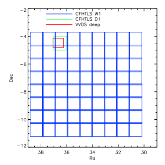
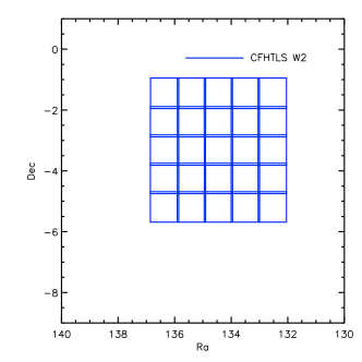
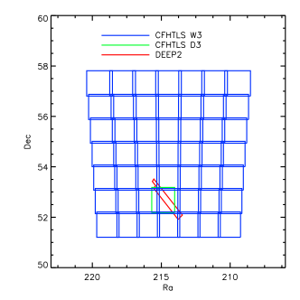
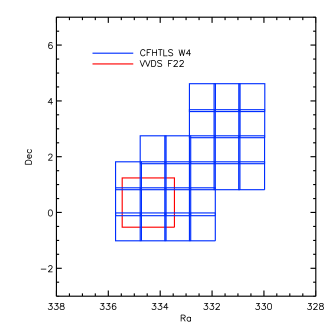
We use the “T0006” release of the CFHTLS Wide111http://terapix.iap.fr/cplt/T0006-doc.pdf (Goranova et al., 2009). The CFHTLS Wide has the mean limiting AB magnitudes (measured as the 50% completeness for point sources) 25.3,25.5,24.8,24.48,23.60similar-toabsent25.325.524.824.4823.60\sim 25.3,25.5,24.8,24.48,23.60 in u,g,r,i,zsuperscript𝑢superscript𝑔superscript𝑟superscript𝑖superscript𝑧u^{\ast},g^{\prime},r^{\prime},i^{\prime},z^{\prime}, respectively. An important feature in T0006 compared to previous releases is that for each MegaCam pointing (“tile”), the TERAPIX group provides a magnitude offset in each filter to account for tile-to-tile variations in magnitude zero points. These offsets are calculated using a stellar locus regression technique (High et al., 2009). In each tile, objects are detected on a gri𝑔𝑟𝑖gri-χ2superscript𝜒2\chi^{2} image (Szalay et al., 1999). Galaxies are selected using SEXtractormag_auto” magnitudes (Bertin & Arnouts, 1996), and colours are measured in 333\arcsec apertures which are all well matched to the median size of galaxies at our i<22.5superscript𝑖22.5i^{\prime}<22.5 magnitude limit. The sky coverage of the four CFHTLS Wide fields is shown in Figure 1.

The MegaCam i𝑖i-band filter broke in 2006, and subsequent observations were made with a new i𝑖i-band filter denoted by “y𝑦y”. Data from these two filters were treated separately with separate filter curves. Using a small data set observed with both the new y𝑦y- and the old i𝑖i-band, we detected no significant difference in photometric redshift accuracy. For the rest of the paper, we use isuperscript𝑖i^{\prime} to represent both filters.

Refer to caption Refer to caption
Figure 1: Sky coverage of W1,W2,W3 and W4 fields. Each blue square represents one MegaCam pointing. Spectroscopic data (VVDS F02, F22, and DEEP2) are in red. CFHTLS Deep fields overlapping with the wide survey (D1 and D3) are shown in green.

2.2 Photometric redshift estimation

Our photometric redshifts were measured using LePhare (Arnouts et al., 2002) following the procedures outlined in Ilbert et al. (2006) and Coupon et al. (2009). Our primary template set is composed of the four Coleman et al. (1980) (CWW) observed spectra (Ell, Sbc, Scd, Irr) complemented with two observed starburst spectral energy distributions (SED) from Kinney et al. (1996). This primary set of templates is optimized using the VVDS Deep spectroscopic sample. We performed an automatic calibration of the zero-points using spectroscopic redshifts in the W1, W3 and W4 fields. The calibration is obtained by comparing the observed and modelled fluxes, and done iteratively until the zero-points converge. For spectral types later than Sbc, we introduced a reddening E(BV)=0𝐸𝐵𝑉0E(B-V)=0 to 0.350.350.35 using the Calzetti et al. (2000) extinction law.

Without near-infrared photometry, Lyman- and Balmer- breaks create degeneracies between high and low photometric redshift solutions. Following a Bayesian approach similar to Benítez (2000) and Ilbert et al. (2006), we adopt a “prior” based on the observed spectroscopic redshift distribution to reduce the number of catastrophic failures. No redshift solution is allowed which will produce a galaxy brighter than Mg=24subscript𝑀𝑔24M_{g}=-24.

Our photometric redshifts were calibrated with spectroscopic samples. The VVDS Deep survey (Le Fèvre et al., 2005) is available in the W1 field. The VVDS Deep is a pure magnitude-limited sample at IAB<24subscript𝐼AB24I_{\rm AB}<24 and we used 5 92659265\,926 secure redshifts (flags 4 and 5) for photometric calibration, and for building the redshift distribution prior. From the VVDS F22 (“VVDS WIDE”, Garilli et al., 2008) in W4 we used 4 51445144\,514 galaxies limited to IAB<22.5subscript𝐼AB22.5I_{\rm AB}<22.5. This sample has a success rate of 92%. Finally, in the W3 field, 1 26712671\,267 redshifts from the DEEP2 survey (Davis et al., 2003) selected at RAB<24.1subscript𝑅AB24.1R_{\rm AB}<24.1 were used for photometric calibration. No spectroscopic redshifts were available in W2.

To estimate photometric redshifts, we adopted a slightly different method than for previous studies to measure redshifts from the probability distribution function (PDF). Rather than directly using the redshift that minimizes the χ2superscript𝜒2\chi^{2} distribution function, we chose the median of the PDF. It has been found that the maximum likelihood estimate can lead to a systematic concentration of photometric redshifts around discrete values (“redshift focusing”), although we checked that the effect is very small for redshift bins of size Δz>0.1Δ𝑧0.1\Delta z>0.1.

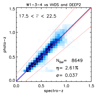
The redshift accuracy (“σ𝜎\sigma”) of our samples with spectroscopic redshift zssubscript𝑧sz_{\rm s} and photometric redshift zpsubscript𝑧pz_{\rm p} is defined as σΔz/(1+zs)subscript𝜎subscriptΔ𝑧1subscript𝑧s\sigma_{\Delta_{z}}/(1+z_{\rm s}), where Δz=|zpzs|Δ𝑧subscript𝑧psubscript𝑧s\Delta z=|z_{\rm p}-z_{\rm s}| represents the difference between spectroscopic and photometric redshift. We use the normalised median absolute deviation as accuracy estimator (NMAD, Hoaglin et al., 1983), expressed as σΔz=1.48×median(|zpzs|)subscript𝜎subscriptΔ𝑧1.48mediansubscript𝑧psubscript𝑧s\sigma_{\Delta_{z}}=1.48\times{\rm median}(|z_{\rm p}-z_{\rm s}|). “Catastrophic” redshifts are defined as objects with |zpzs|/(1+zs)>0.15subscript𝑧psubscript𝑧s1subscript𝑧s0.15|z_{\rm p}-z_{\rm s}|/(1+z_{\rm s})>0.15. The percentage of catastrophic redshifts is denoted by η𝜂\eta. The dispersion and the fraction of catastrophic redshifts increase from bright to faint samples. The accuracy is σΔz/(1+zs)=0.034subscript𝜎subscriptΔ𝑧1subscript𝑧s0.034\sigma_{\Delta_{z}}/(1+z_{\rm s})=0.034 (W1) to 0.0370.0370.037 (W4) at i<21.5superscript𝑖21.5i^{\prime}<21.5 and reaches 0.0390.0390.039 (W1) to 0.0510.0510.051 (W3) at 21.5<i<22.521.5superscript𝑖22.521.5<i^{\prime}<22.5. The failure rate increases from η1.4%similar-to𝜂percent1.4\eta\sim 1.4\% at i<21.5superscript𝑖21.5i^{\prime}<21.5 to η5.5%similar-to𝜂percent5.5\eta\sim 5.5\% at 21.5<i<22.521.5superscript𝑖22.521.5<i^{\prime}<22.5. Galaxies with redder colours (El, Sbc) have more accurate photometric redshift estimates (σΔz/(1+zs)=0.031subscript𝜎subscriptΔ𝑧1subscript𝑧s0.031\sigma_{\Delta_{z}}/(1+z_{\rm s})=0.031, η=1.64%𝜂percent1.64\eta=1.64\%) than bluer ones (Scd, Irr and starbursts, σΔz/(1+zs)=0.038subscript𝜎subscriptΔ𝑧1subscript𝑧s0.038\sigma_{\Delta_{z}}/(1+z_{\rm s})=0.038, η=3.69%𝜂percent3.69\eta=3.69\%).

We constructed a merged catalogue with unique objects from individual tile catalogues provided by TERAPIX. We identified duplicate sources positionally and chose the object closest to the centre of its original tile. Although photometric redshifts were estimated to i<24superscript𝑖24i^{\prime}<24, we selected objects brighter than i=22.5superscript𝑖22.5i^{\prime}=22.5 to maintain a low outlier rate (see Table 3 of Coupon et al., 2009) and to ensure catalogue completeness. This sample covers a total effective area of 133 deg2. We show the photometric redshift accuracy in the secure redshift range covered in this study, 0.2<z<1.20.2𝑧1.20.2<z<1.2, compared to spectroscopic redshifts in Fig. 2.

Stars appear as point-like sources on the image and can easily be identified using their half-light radius at bright magnitudes; however, at fainter magnitudes this estimator can be confused by unresolved galaxies. We refined our star-galaxy separation by combining this profile-magnitude criteria with a colour-based criteria. We computed the half-light radius limit for each tile from the median and dispersion of the brightest objects and classified as stars all objects brighter than i=20superscript𝑖20i^{\prime}=20 with flux radii limits smaller than this amount. In the magnitude range 20<i<22.520superscript𝑖22.520<i^{\prime}<22.5, we classified stars as objects smaller than the half-light radius and with χ2(star)<χ2(galaxy)superscript𝜒2starsuperscript𝜒2galaxy\chi^{2}({\rm star})<\chi^{2}({\rm galaxy}), where χ2(object)superscript𝜒2object\chi^{2}({\rm object}) is estimated from the stellar and galaxy template libraries.

We eliminated objects observed with less than three filters and with χ2(galaxy)>100superscript𝜒2galaxy100\chi^{2}({\rm galaxy})>100. We suspect that these objects are false detections or rare objects with wrong photometric redshift estimates. Most of these objects reside in specific areas, such as around bright stars and field borders where the masking procedure has failed.

Using the photometric redshift, the associated best-fitting template and the observed apparent magnitude in a given band, we can directly measure the klimit-from𝑘k-correction and the absolute magnitude in any rest-frame band. Since at high redshifts the klimit-from𝑘k-correction depends strongly on the galaxy spectral energy distribution, it is the main source of systematic error in determining absolute magnitudes. To minimise klimit-from𝑘k-correction uncertainties, we derive the rest-frame luminosity at λ𝜆\lambda using the object’s apparent magnitude closer to λ×(1+z)𝜆1𝑧\lambda\times(1+z). We use either the uu*, gsuperscript𝑔g^{\prime}, rsuperscript𝑟r^{\prime}, isuperscript𝑖i^{\prime}, or zsuperscript𝑧z^{\prime} observed apparent magnitudes according to the redshift of the galaxy (the procedure is described in Appendix A of Ilbert et al., 2005). For this reason the bluest absolute magnitude estimate makes full advantage of the complete observed magnitude set. However, as the ulimit-from𝑢u-band flux has larger photometric errors, we decided to use Mgsubscript𝑀𝑔M_{g}-band magnitudes.

Refer to caption
Figure 2: Photometric redshift accuracy in the 0.2<photoz<1.20.2photo𝑧1.20.2<{\rm photo-}z<1.2 interval. The figure shows the number density of photometric redshifts in W1, W3 and W4, versus spectroscopic redshifts from VVDS and DEEP2 surveys. The blue line is a linear fit to photo-z versus spectro-z.

3 Clustering measurements

3.1 Sample selection and galaxy number density estimation

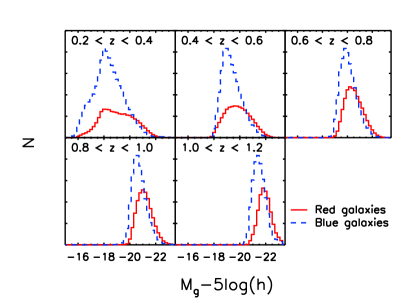
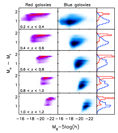
Objects are selected with i<22.5superscript𝑖22.5i^{\prime}<22.5 and divided into five redshift bins: 0.2<z<0.40.2𝑧0.40.2<z<0.4, 0.4<z<0.60.4𝑧0.60.4<z<0.6, 0.6<z<0.80.6𝑧0.80.6<z<0.8, 0.8<z<1.00.8𝑧1.00.8<z<1.0, and 1.0<z<1.21.0𝑧1.21.0<z<1.2. A large bin width (Δz=0.2subscriptΔ𝑧0.2\Delta_{z}=0.2) ensures a low bin-to-bin contamination from random errors (σz<0.1subscript𝜎𝑧0.1\sigma_{z}<0.1). We investigate effects from systematic errors in Sect. 3.2. The complete sample contains 2 924 73029247302\,924\,730 galaxies. To separate galaxies into “red sequence” and “blue cloud” types, we used a criterion based on best-fitting galaxy templates. We define “red” galaxies as objects with best-fitting CWW templates (see Sect. 2.2) estimated as El and Sbc (early-type), and “blue” galaxies estimated as Sbc, Scd, Im, SB1 and SB2 (late-type). Selecting galaxies by best-fitting template is a more robust way of selecting galaxies by type, as compared to a simple colour selection, and it is less sensitive to the effects of dust extinction. Our resulting colour selection in the absolute magnitude-redshift plane is shown in Fig. 3. We note that a small amount of red-classified galaxies at high redshift z>0.8𝑧0.8z>0.8 have slightly bluer colours. Their distribution peaks near the blue galaxy distribution, suggesting that these objects could be blue galaxies erroneously identified as red galaxies due to photometric redshift errors. We also note that a simple colour cut would not exactly reproduce our selection. However, in the interests of simplicity and clarity we keep the “red”/”blue” labels for the rest of the paper.
Refer to caption
Refer to caption
Figure 3: Top: type selection based on best fitting templates for the “red” sample (left) and the “blue” sample (right) in the CFHTLS Wide. We show the colour distribution (MuMrsubscript𝑀𝑢subscript𝑀𝑟M_{u}-M_{r}) as function of absolute magnitude (Mgsubscript𝑀𝑔M_{g}) and redshift (top to bottom) and number counts for “red” and “blue” objects on the right panels. Bottom: number of red and blue galaxies as function of magnitude and redshift.

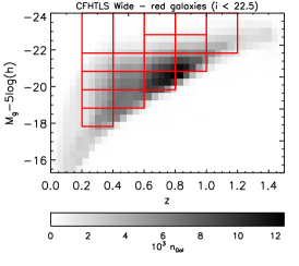
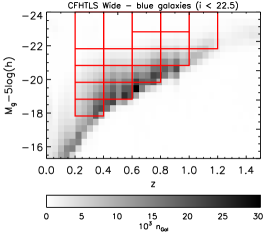
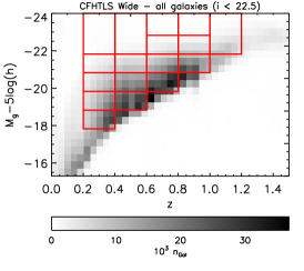
We extract volume-limited luminosity-selected samples for each of the “full” (or “all galaxies”), “red” and “blue” samples, using Mgsubscript𝑀𝑔M_{g} absolute magnitude thresholds (hereafter denoted as “luminosity threshold samples”), from Mg5logh=17.8subscript𝑀𝑔517.8M_{g}-5\log h=-17.8 (fainter threshold in the range 0.2<z<0.40.2𝑧0.40.2<z<0.4) to Mg5logh=22.8subscript𝑀𝑔522.8M_{g}-5\log h=-22.8 (brighter threshold in the range 1.0<z<1.21.0𝑧1.21.0<z<1.2). The sample selection is illustrated in Fig. 4. For the rest of this paper we will refer to these samples as simply full, red and blue.
Refer to caption Refer to caption Refer to caption
Figure 4: Sample selection in the full (left), red (center) and blue (right) galaxy samples. In each panel, the galaxy number density in the plane Mg/zsubscript𝑀𝑔𝑧M_{g}/z is shown; red rectangles represent the luminosity threshold samples.

Due to low numbers of pairs at small scales, luminous blue samples were discarded. We are left with 45 samples, each comprising on average 153 000similar-toabsent153000\sim 153\,000, 70 000similar-toabsent70000\sim 70\,000 and 129 000similar-toabsent129000\sim 129\,000 galaxies for a typical full, red and blue sample, respectively. The sample properties are displayed in Tables 1, 2 and 3.

Finally, in each redshift interval [zmin;zmax]subscript𝑧minsubscript𝑧max[z_{\rm min};z_{\rm max}] we compute the galaxy number density:

ngalobs=Ntotal/[ΩzminzmaxdVdzdz],superscriptsubscript𝑛galobssubscript𝑁totaldelimited-[]Ωsuperscriptsubscriptsubscript𝑧minsubscript𝑧maxd𝑉d𝑧differential-d𝑧n_{\rm gal}^{\rm obs}={N_{\rm total}}/\left[{\Omega\int_{z_{\rm min}}^{z_{\rm max}}\frac{\mathrm{d}V}{\mathrm{d}z}\,\mathrm{d}z}\right], (1)

where ΩΩ\Omega represents the solid angle subtended by the survey, and dV/dzd𝑉d𝑧\mathrm{d}V/\mathrm{d}z the volume element. Errors are estimated from the weighted galaxy number density field-to-field variance.

3.2 Photometric redshift uncertainties

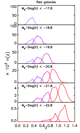
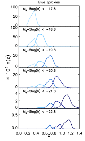
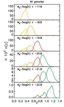
Our modelled two-point correlation function is projected using the measured redshift distributions. In order to take into account statistical errors on redshifts, we select galaxies in the redshift range considered and convolve the observed redshift distributions with the estimated photometric redshift errors, derived from the probability distribution functions. We construct a Gaussian error distribution for each galaxy centred on the median redshift of the PDF, with a width corresponding to the 68% confidence limits of the PDF, and normalised to unity. We then sum these Gaussians to construct the redshift distribution resampled to a redshift bin width of 0.04. Redshift distributions for each sample are illustrated in Fig. 5.
Refer to caption Refer to caption Refer to caption
Figure 5: Redshift distributions for the full (left), red (center) and blue (right) galaxy samples as function of absolute magnitude threshold.

To further assess the quality of photometric redshifts, we perform the cross-correlation analysis introduced in Benjamin et al. (2010). The measurement of the angular correlation functions for galaxies in different photo-z𝑧z bins is used to constrain the fraction of galaxies that are scattered into “wrong” redshift bins due to photo-z𝑧z errors. We measure the bin-to-bin cross correlation function for the full, red and blue samples, respectively. A non-zero correlation between adjacent redshift bins is present in all cases. This may be due to the presence of large-scale structures extending over several redshift bins. More importantly, this is also due to photometric redshift scatter, which results in the leakage of galaxies into neighbouring bins. This error contribution to the redshifts is taken into account by the convolution of the redshift distribution with the errors, therefore, we do not consider adjacent bins further in the analysis of photometric redshifts uncertainties.

The angular cross-correlation of galaxies in non-adjacent redshift bins is much lower, indicating a small fraction of catastrophic outliers. We use the “global pairwise analysis” method to measure the contamination between two redshift bins i𝑖i and j𝑗j. In this approximation, the following linear combinations of the angular cross-correlation function wijsubscript𝑤𝑖𝑗w_{ij} and the two auto-correlation functions, wiisubscript𝑤𝑖𝑖w_{ii} and wjjsubscript𝑤𝑗𝑗w_{jj}, respectively, are expected to cancel for all angular scales θtsubscript𝜃𝑡\theta_{t},

dtsubscript𝑑𝑡\displaystyle d_{t} =\displaystyle= wij(θt)(fiifjj+fijfji)wii(θt)NiNjfijfjjwjj(θt)NjNifjifiisubscript𝑤𝑖𝑗subscript𝜃𝑡subscript𝑓𝑖𝑖subscript𝑓𝑗𝑗subscript𝑓𝑖𝑗subscript𝑓𝑗𝑖subscript𝑤𝑖𝑖subscript𝜃𝑡subscript𝑁𝑖subscript𝑁𝑗subscript𝑓𝑖𝑗subscript𝑓𝑗𝑗subscript𝑤𝑗𝑗subscript𝜃𝑡subscript𝑁𝑗subscript𝑁𝑖subscript𝑓𝑗𝑖subscript𝑓𝑖𝑖\displaystyle w_{ij}(\theta_{t})\left(f_{ii}f_{jj}+f_{ij}f_{ji}\right)-w_{ii}(\theta_{t})\frac{N_{i}}{N_{j}}f_{ij}f_{jj}-w_{jj}(\theta_{t})\frac{N_{j}}{N_{i}}f_{ji}f_{ii} (2)
=\displaystyle= 0.0\displaystyle 0.

Here, Ni(Nj)subscript𝑁𝑖subscript𝑁𝑗N_{i}\;(N_{j}) is the observed number of galaxies in bin i(j)𝑖𝑗i\;(j). The contamination fijsubscript𝑓𝑖𝑗f_{ij} is the number of galaxies with true redshift in bin i𝑖i, but misidentified into bin j𝑗j, as a fraction of the true number of galaxies in bin i𝑖i. For each bin pair (i,j𝑖𝑗i,j), the leakage of the other redshift bins is neglected. This approximation is valid for contamination fractions of up to 10% (Benjamin et al., 2010). With this, the fraction of galaxies which stay in their bin is fii=1fijsubscript𝑓𝑖𝑖1subscript𝑓𝑖𝑗f_{ii}=1-f_{ij}. We fit the two parameters fijsubscript𝑓𝑖𝑗f_{ij} and fjisubscript𝑓𝑗𝑖f_{ji} in Eq. 2 by performing a χ2superscript𝜒2\chi^{2} null-test on dtsubscript𝑑𝑡d_{t}. For the covariance dtdsdelimited-⟨⟩subscript𝑑𝑡subscript𝑑𝑠\langle d_{t}d_{s}\rangle, we take into account the correlation between angular scales for each of the three correlation functions using a Jackknife estimate (see next section). We neglect the sub-dominant covariance between different correlation functions. This corresponds to using the first three terms in Eq. A4 of Benjamin et al. (2010).

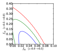
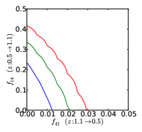
Due to degeneracies between the parameters fijsubscript𝑓𝑖𝑗f_{ij} and fjisubscript𝑓𝑗𝑖f_{ji}, large values for fij(i>j)subscript𝑓𝑖𝑗𝑖𝑗f_{ij}\;(i>j) cannot be ruled out in principle. However, for the full and red galaxy samples, the contamination fractions are consistent with zero in most cases. The blue galaxy samples are slightly worse, but contaminations are consistent with values between 2% and 10%. Together with the very low outlier rate for the sub-sample with spectroscopic redshifts (see Fig. 2), these results further strengthen our confidence in the photometric redshift estimates in this work and to use them to measure angular correlation functions. Our measurements for the full sample are shown in Fig. 6.

Refer to caption
Refer to caption Refer to caption
Figure 6: Cross correlation analysis between redshift bins for the full sample. Top: auto-correlation in the redshift bin 0.4<z<0.60.4𝑧0.60.4<z<0.6 (straight line) and cross-correlation between the bins 0.4<z<0.60.4𝑧0.60.4<z<0.6 and 0.8<z<1.00.8𝑧1.00.8<z<1.0 (dotted line) and between 0.4<z<0.60.4𝑧0.60.4<z<0.6 and 1.0<z<1.21.0𝑧1.21.0<z<1.2 (dashed line). Bottom: quantitative estimates of the contamination (percentage of galaxies scattered) from a pairwise analysis between redshift bins 0.4<z<0.60.4𝑧0.60.4<z<0.6 and 0.8<z<1.00.8𝑧1.00.8<z<1.0 (left) and between 0.4<z<0.60.4𝑧0.60.4<z<0.6 and 1.0<z<1.21.0𝑧1.21.0<z<1.2 (right). The contours show the 68.3 (blue), 95.5 (green) and 99.7 (red) confidence regions.

Bin-to-bin mixing caused by photometric redshift errors will reduce our measured clustering signal, given that objects in separate bins are uncorrelated. This would lead to an underestimation of halo masses, as low mass haloes tend to be less clustered than more massive ones. However, it is not trivial to predict how galaxy number density estimates would be affected by such errors, which may result in incomplete or contaminated samples. Since the halo number density decreases monotonically with halo mass, galaxy number density decreases with increasing host halo mass. Therefore, a contaminated sample will underestimate halo mass fitting estimates. Conversely, an incomplete sample will tend to overestimate halo masses.

To understand how photometric redshift errors could affect our results as function of redshift and luminosity threshold, we compared our measurements in the CFHTLS Wide with those from the “Deep” component of the CFHTLS (Goranova et al., 2009), where more precise photometric redshifts are available (see Table 3 in Coupon et al., 2009). Photometric redshifts in the CFHTLS Deep were computed using the method described in Sect. 2.2 and to avoid cosmic variance uncertainties we performed our tests in overlapping areas between the Wide and the Deep, D1/W1 and D3/W3, over a total area of 2 deg2.

These tests show that faint luminosity threshold samples are slightly incomplete at low redshift, probably as a consequence of catastrophic errors moving low redshift galaxies to higher redshift. We report that the difference in galaxy density between the Wide and the Deep estimates rarely exceeds the field-to-field variance error estimate. However, brighter and brighter samples become more and more contaminated by spurious objects, and in the worst case (the brightest sample in the range 0.8<z<1.00.8𝑧1.00.8<z<1.0), the number of objects in the Wide is more than three times higher than in the Deep, much larger than the 40% field-to-field variance. A higher galaxy number density estimate will enhance the effect of a reduced clustering signal, which may result in underestimated halo masses for brighter samples up to a few sigmas. In the worst case, this represents a bias of 0.5similar-toabsent0.5\sim 0.5 in logMminsubscript𝑀min\log M_{\rm min}.

3.3 Angular correlation function

We measure the two-point angular correlation function w𝑤w using the Landy & Szalay (1993) estimator

w(θ)=Nr(Nr1)Nd(Nd1)DDRRNr1NdDRRR+1,𝑤𝜃subscript𝑁rsubscript𝑁r1subscript𝑁dsubscript𝑁d1delimited-⟨⟩𝐷𝐷delimited-⟨⟩𝑅𝑅subscript𝑁r1subscript𝑁ddelimited-⟨⟩𝐷𝑅delimited-⟨⟩𝑅𝑅1w(\theta)=\frac{N_{\rm r}(N_{\rm r}-1)}{N_{\rm d}(N_{\rm d}-1)}\frac{\langle DD\rangle}{\langle RR\rangle}-\frac{N_{\rm r}-1}{N_{\rm d}}\frac{\langle DR\rangle}{\langle RR\rangle}+1\,, (3)

where DDdelimited-⟨⟩𝐷𝐷\langle DD\rangle is the number of galaxy pairs, RRdelimited-⟨⟩𝑅𝑅\langle RR\rangle the number of random pairs, DRdelimited-⟨⟩𝐷𝑅\langle DR\rangle the number of galaxy-random pairs, all in a bin around the angular separation θ𝜃\theta. Ndsubscript𝑁dN_{\rm d} and Nrsubscript𝑁rN_{\rm r} are the number of galaxies and random objects, respectively. A random catalogue is generated for each sample. In order to find an acceptable compromise between small Poisson errors and computational requirements we scale Nrsubscript𝑁rN_{\rm r} depending on the number of galaxies in our input catalogues, from 50×Nd50subscript𝑁d50\times N_{\rm d} in the case of low density data catalogues to 2×Nd2subscript𝑁d2\times N_{\rm d} for high density catalogues. We measure w𝑤w using a fast two-dimensional tree code. At large separations θ𝜃\theta, instead of counting individual galaxy pairs, we correlate boxes by multiplying the number of objects in the two boxes. For that, we define a threshold angle αw=θ/dbsubscript𝛼𝑤𝜃subscript𝑑b\alpha_{w}=\theta/d_{\rm b}, where dbsubscript𝑑bd_{\rm b} is the box size. Below this threshold, the number of objects inside the box is taken into account instead of individual objects. We found that αw=0.05subscript𝛼𝑤0.05\alpha_{w}=0.05 gives accurate results at low computational cost.

We correct our galaxy correlation measurements for the “integral constraint” (Groth & Peebles, 1977), a correction factor which arises from the finite area of our survey Ω2superscriptΩ2\Omega^{2}:

w(θ)=wmes(θ)+wC.𝑤𝜃subscript𝑤mes𝜃subscript𝑤𝐶w(\theta)=w_{\rm mes}(\theta)+w_{C}\,. (4)

The correction factor wCsubscript𝑤𝐶w_{C} can be estimated as follows:

wC=1Ω2w(θ)dΩ1dΩ2,subscript𝑤𝐶1superscriptΩ2𝑤𝜃differential-dsubscriptΩ1differential-dsubscriptΩ2w_{C}=\frac{1}{\Omega^{2}}\int\!\!\!\!\int w(\theta)\,\mathrm{d}\Omega_{1}\mathrm{d}\Omega_{2}\,, (5)

assuming a simple power law fitted on the data with slope γ𝛾\gamma and amplitude Awsubscript𝐴𝑤A_{w}:

wmes(θ)=Awθ1γwC=Aw(θ1γC).subscript𝑤mes𝜃subscript𝐴𝑤superscript𝜃1𝛾subscript𝑤𝐶subscript𝐴𝑤superscript𝜃1𝛾𝐶w_{\rm mes}(\theta)=A_{w}\theta^{1-\gamma}-w_{C}=A_{w}(\theta^{1-\gamma}-C)\,. (6)

As Awsubscript𝐴𝑤A_{w} varies with each sample, we first compute C using Monte Carlo integration over random pairs

C=θ1γRR(θ)RR(θ),𝐶superscript𝜃1𝛾𝑅𝑅𝜃𝑅𝑅𝜃C=\frac{\sum\theta^{1-\gamma}RR(\theta)}{\sum RR(\theta)}\,, (7)

and then correct wmes(θ)subscript𝑤mes𝜃w_{\rm mes}(\theta) using

w(θ)=wmes(θ)θ1γθ1γC.𝑤𝜃subscript𝑤mes𝜃superscript𝜃1𝛾superscript𝜃1𝛾𝐶w(\theta)=w_{\rm mes}(\theta)\frac{\theta^{1-\gamma}}{\theta^{1-\gamma}-C}\,. (8)

The integral constraint for the four Wide fields is C0.5similar-to𝐶0.5C\sim 0.5. Assuming γ=1.8𝛾1.8\gamma=1.8, this leads to a correction of 10%similar-toabsentpercent10\sim 10\% at θ=0.1𝜃0.1\theta=0.1 deg and up to a factor of two at θ=1.0𝜃1.0\theta=1.0 deg. We note that assuming a power-law for w(θ)𝑤𝜃w(\theta) to estimate C𝐶C could be a source of error; it is neglected in the current analysis as the correction is smaller than our Jackknife error estimates.

We combine our galaxy samples from the four CFHTLS fields into a single catalogue for the correlation function measurement. Computing w(θ)𝑤𝜃w(\theta) on the four fields independently, and using a pair-weighted average would not lead to the same clustering estimate at large scales. Relative photometric offsets are expected to vary more from one field to another than within the same field, as the four fields are non-overlapping. Since our parent catalogue is selected by apparent magnitude cut (i<22.5superscript𝑖22.5i^{\prime}<22.5), even a small difference in photometric offsets will lead to a spurious field-to-field variation of the galaxy number density. In addition, different photometric offsets could bias the photometric redshift selection and also increase the field-to-field density fluctuations. A 0.02 magnitude offset variation would result in a 2%similar-toabsentpercent2\sim 2\% variation in galaxy number density, which may bias the two-point correlation at very large scales. Because we expect these effects to occur at the scale of individual field (a few degrees), we adopt a conservative cut and limit our measurements to θ<1.5deg𝜃1.5degree\theta<1.5\deg. We do not measure w𝑤w at separations below 3.63\aas@@fstack{\prime\prime}6 to avoid blended objects. Two-point correlation function measurements and errors are provided in the appendix C.

3.4 w(θ)𝑤𝜃w(\theta) error estimates

We estimate statistical errors on the two-point correlation function using the Jackknife internal estimator. We divide all samples into N=68𝑁68N=68 sub-samples of about 2deg22superscriptdegree22\deg^{2}. Removing one sub-sample at a time for each Jackknife realisation, we compute the covariance matrix as

C(wi,wj)=N1Nl=1N(wilw¯i)(wjlw¯j),Csubscript𝑤𝑖subscript𝑤𝑗𝑁1𝑁superscriptsubscript𝑙1𝑁superscriptsubscript𝑤𝑖𝑙subscript¯𝑤𝑖superscriptsubscript𝑤𝑗𝑙subscript¯𝑤𝑗\mathrm{C}(w_{i},w_{j})=\frac{N-1}{N}\sum_{l=1}^{N}(w_{i}^{l}-\overline{w}_{i})(w_{j}^{l}-\overline{w}_{j})\,, (9)

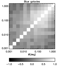
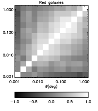
where N𝑁N is the total number of subsamples, w¯¯𝑤\overline{w} the mean correlation function, and wlsuperscript𝑤𝑙w^{l} the estimate from the lthsuperscript𝑙thl^{\rm th} Jackknife sample. Since w(θ)𝑤𝜃w(\theta) is computed from a combined catalogue including all four fields, our Jackknife estimate leads to a noisy but fair estimate of cosmic variance. We apply the correction factor given by Hartlap et al. (2007) to the inverse covariance matrix to compensate for the bias introduced by the noise. We show the correlation coefficient of the covariance matrix, rij=Cij/CiiCjjsubscript𝑟𝑖𝑗subscript𝐶𝑖𝑗subscript𝐶𝑖𝑖subscript𝐶𝑗𝑗r_{ij}=C_{ij}/\sqrt{C_{ii}C_{jj}} for two red and blue samples, respectively, in Fig. 7.
Refer to caption
Refer to caption
Figure 7: Covariance matrix correlation coefficients of w(θ)𝑤𝜃w(\theta) from Jackknife estimates, for galaxy samples with 0.4<z<0.60.4𝑧0.60.4<z<0.6 and Mg5logh<19.8subscript𝑀𝑔519.8M_{g}-5\log h<-19.8. Left panel: red sample. Right panel: blue sample.

4 Filling haloes with galaxies: the halo occupation model

4.1 The halo occupation distribution

In order to relate galaxies to the dark matter haloes which host them we have implemented an analytic model of galaxy clustering, the halo model (for a review see Cooray & Sheth, 2002), which contains at its core a prescription for how galaxies populate haloes, namely the halo occupation distribution. Our model follows closely the approaches used in recent works; further details and references can be found in Appendix A. The key assumption underlying our halo occupation distribution function is that the number of galaxies N𝑁N in a given dark matter halo depends only on the halo mass M𝑀M; it does not depend on environment of formation history of the haloes. Furthermore, following Zheng et al. (2005), we express N(M)𝑁𝑀N(M) as the sum of two terms, corresponding to the contribution from the central galaxy Ncsubscript𝑁cN_{\rm c} and the satellite galaxies Nssubscript𝑁sN_{\rm s}:

N(M)=Nc(M)×[1+Ns(M)],𝑁𝑀subscript𝑁c𝑀delimited-[]1subscript𝑁s𝑀N(M)=N_{\rm c}(M)\times\left[1+N_{\rm s}(M)\right]\,, (10)

where

Nc(M)subscript𝑁c𝑀\displaystyle N_{\rm c}(M) =\displaystyle= 12[1+erf(logMlogMminσlogM)],12delimited-[]1erf𝑀subscript𝑀minsubscript𝜎𝑀\displaystyle\frac{1}{2}\left[1+\mathrm{erf}\left(\frac{\log M-\log M_{\rm min}}{\sigma_{\log M}}\right)\right]\,, (11)
Ns(M)subscript𝑁s𝑀\displaystyle N_{\rm s}(M) =\displaystyle= (MM0M1)α.superscript𝑀subscript𝑀0subscript𝑀1𝛼\displaystyle\left(\frac{M-M_{0}}{M_{1}}\right)^{\alpha}\,. (12)

The smooth transition for central galaxies expresses the uncertainties in the galaxy formation process (Zheng et al., 2007). The factor Nc(M)subscript𝑁c𝑀N_{\rm c}(M) for the satellite number in N(M)𝑁𝑀N(M) accounts for the fact that a halo cannot be populated by satellite galaxies without the presence of a central galaxy.

For a given cosmology and dark matter halo profile, our model has five adjustable parameters. Mminsubscript𝑀minM_{\rm min} is the mass scale for which 50% of haloes host a galaxy. To reflect the scatter in the luminosity-halo mass relation, a smooth transition of width σlogMsubscript𝜎𝑀\sigma_{\log M} is used. Zheng et al. (2007) show that if this scatter is small, the above expression takes the identical form as the distribution of central galaxies given a halo mass M𝑀M, integrated over the entire luminosity range above the luminosity threshold. Thus Mminsubscript𝑀minM_{\rm min} also represents the halo mass scale for central galaxies, whose mean luminosity Lcdelimited-⟨⟩subscript𝐿c\langle L_{\rm c}\rangle is equal to the luminosity threshold Lminsubscript𝐿minL_{\rm min}.

This simple relation between Mminsubscript𝑀minM_{\rm min} and Lcsubscript𝐿cL_{\rm c} is based on the hypothesis that stellar mass (or luminosity) has a power law dependence on halo mass, which may not be exact over the entire mass range. Leauthaud et al. (2011a) recently proposed a model in which this relation assumes a more realistic form. The authors showed that in their model Mminsubscript𝑀minM_{\rm min} and σlogMsubscript𝜎𝑀\sigma_{\log M} take different values than those computed with other models. However, in the mass range over which we compare our results with theirs in Sect. 6 (Mh1012h1Msimilar-tosubscript𝑀hsuperscript1012superscript1subscript𝑀direct-productM_{\rm h}\sim 10^{12}h^{-1}M_{\odot}), Mminsubscript𝑀minM_{\rm min} values do not differ by more than 10% (see Fig. 3 in Leauthaud et al., 2011a).

The number of satellite galaxies as function of halo mass follows a power law with slope α𝛼\alpha and amplitude M1subscript𝑀1M_{1}. M1subscript𝑀1M_{1} then represents the characteristic scale for haloes hosting one satellite galaxy. At lower masses, the dependence becomes steeper and the transition mass scale occurs at MM0similar-to𝑀subscript𝑀0M\sim M_{0}.

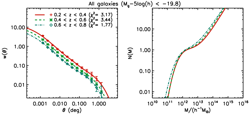
We show in Fig. 8 an example of measured w(θ)𝑤𝜃w(\theta) and its best-fitting model, together with the best-fitting HOD function N(M)𝑁𝑀N(M). The total galaxy correlation function is the sum of two terms. At distances much smaller than the virial radius, the one-halo term contains contributions from galaxy pairs within a single halo, whereas at large distances the two-halo term contains contributions from pairs in separate haloes.

Refer to caption
Figure 8: Example of a measured w(θ)𝑤𝜃w(\theta) (for all galaxies in the redshift range 0.4<z<0.60.4𝑧0.60.4<z<0.6 and for Mg5logh<19.8𝑀𝑔519.8Mg-5\log h<-19.8), as well as the best-fitting model, as described in sec. 4. Left: w(θ)𝑤𝜃w(\theta) measurement and model. Right: N(M)𝑁𝑀N(M), showing the central term Ncentsubscript𝑁𝑐𝑒𝑛𝑡N_{cent} and the satellite term Nssubscript𝑁sN_{\rm s}.

4.2 Deduced parameters

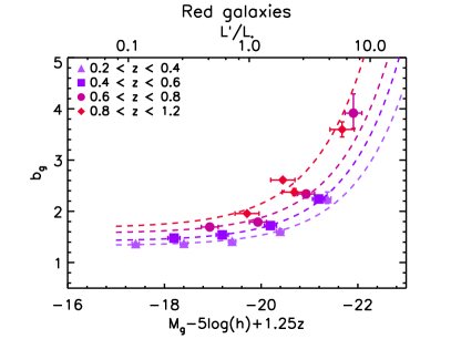
From the HOD model we obtain deduced parameters describing galaxy properties. The mean galaxy bias bgsubscript𝑏gb_{\rm g} at redshift z𝑧z is the mass-integral over the halo bias bhsubscript𝑏hb_{\rm h} (see Sect. A) weighted by the number of galaxies,

bg(z)=dMbh(M,z)n(M,z)N(M)ngal(z).subscript𝑏g𝑧differential-d𝑀subscript𝑏h𝑀𝑧𝑛𝑀𝑧𝑁𝑀subscript𝑛gal𝑧b_{\rm g}(z)=\int\mathrm{d}M\,b_{\rm h}(M,z)\,n(M,z)\frac{N(M)}{n_{\rm gal}(z)}\,. (13)

The dark-matter mass function n𝑛n is given in Eq. 36, and the halo bias bhsubscript𝑏hb_{\rm h} in Eq. 44. The total number of galaxies is

ngal(z)=N(M)n(M,z)dM.subscript𝑛gal𝑧𝑁𝑀𝑛𝑀𝑧differential-d𝑀n_{\rm gal}(z)=\int N(M)\,n(M,z)\,\mathrm{d}M\,. (14)

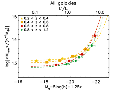
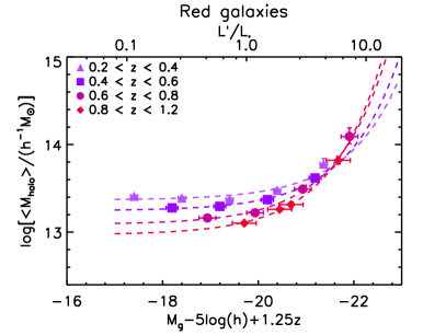
Similarly to the galaxy bias, the mean halo mass for a galaxy population is

Mhalo(z)=dMMn(M,z)N(M)ngal(z).delimited-⟨⟩subscript𝑀halo𝑧differential-d𝑀𝑀𝑛𝑀𝑧𝑁𝑀subscript𝑛gal𝑧\langle M_{\rm halo}\rangle(z)=\int\mathrm{d}M\,M\,n(M,z)\frac{N(M)}{n_{\rm gal}(z)}\,. (15)

The fraction of central galaxies per halo is

fc(z)=dMn(M,z)Nc(M)ngal(z).subscript𝑓c𝑧differential-d𝑀𝑛𝑀𝑧subscript𝑁c𝑀subscript𝑛gal𝑧f_{\rm c}(z)=\int\mathrm{d}M\,n(M,z)\frac{N_{\rm c}(M)}{n_{\rm gal}(z)}\,. (16)

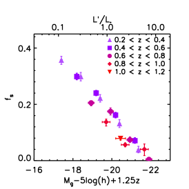
Consequently, the fraction of satellite galaxies is

fs(z)=1fc(z).subscript𝑓s𝑧1subscript𝑓c𝑧f_{\rm s}(z)=1-f_{\rm c}(z)\,. (17)

4.3 Population Monte Carlo sampling

We use the “Population Monte Carlo” (PMC) technique to sample likelihood space (Wraith et al., 2009; Kilbinger et al., 2010, 2011) and have implemented it in a publicly-available code, CosmoPMC222http://cosmopmc.info. Contrary to the widely-used Monte Carlo Markov Chain method (MCMC), PMC is an adaptive importance-sampling technique (Cappé et al., 2004, 2008), which has two principal advantages: first, the parallel sampling algorithm combined with our fast HOD code means that each run can be quickly computed. Secondly, PMC does not have issues with chain convergence. Instead, the perplexity (defined below) is a diagnostic for the reliability of a given sampling run.

Points are sampled from a simple, so-called importance sampling function q𝑞q. Each sample point θnsubscript@vecθ𝑛\@vec{\theta}_{n} is attributed a weight w¯nsubscript¯𝑤𝑛\bar{w}_{n} which is the ratio of the posterior π𝜋\pi to the importance function,

w¯nπ(θn)q(θn);n=1Nw¯n=1.formulae-sequenceproportional-tosubscript¯𝑤𝑛𝜋subscript@vecθ𝑛𝑞subscript@vecθ𝑛superscriptsubscript𝑛1𝑁subscript¯𝑤𝑛1\bar{w}_{n}\propto\frac{\pi(\@vec{\theta}_{n})}{q(\@vec{\theta}_{n})};\;\;\;\sum_{n=1}^{N}\bar{w}_{n}=1. (18)

The initial importance sampling function q𝑞q is a mixture of seven multi-variate Gaussians. A PMC run consists of a number of iterations, in the course of which the importance function is adapted to better match the posterior distribution. We run PMC for typically 10 iterations using 10 0001000010\,000 sample points per iteration.

As a stopping criterion for the iterations we take the perplexity p𝑝p which is defined as

p=1Nexp(n=1Nw¯nlogw¯n).𝑝1𝑁superscriptsubscript𝑛1𝑁subscript¯𝑤𝑛subscript¯𝑤𝑛p=\frac{1}{N}\exp\left(-\sum_{n=1}^{N}\bar{w}_{n}\log\bar{w}_{n}\right). (19)

The perplexity p[0;1]𝑝01p\in[0;1] is a measure of the distance between the posterior and the importance function, and it approaches unity if the two distributions are identical. The perplexity is a measure of the adequacy and efficiency of the sampling. Values of p𝑝p above about 0.6 indicate a good agreement between the posterior and the importance function.

The evaluation of the likelihood function, which is the most time-consuming process for most sampling tasks, is easily parallelisable in importance sampling with little overhead. Furthermore, we have optimized several aspects of the numerical computations of the HOD model. For example, we employ the FFTLog (Hamilton, 2000) algorithm to perform Fourier transforms and make use of tabulated values to improve efficiency. The computation of the angular correlation function w𝑤w on a range of scales is performed in under a second on a standard desktop. This module is part of the latest public version (v1.1) of CosmoPMC. Typically, on an eight-core desktop (16 threads) a single PMC run takes around 90 minutes for a total of 100,000100000100,000 sample points. Our PMC technique allows us to efficiently sample the parameter space for the large number of galaxy samples used in this work.

4.4 Likelihood function

For each galaxy sample we simultaneously fit both the projected angular correlation function w𝑤w and the number density of galaxies ngalsubscript𝑛galn_{\rm gal}, by summing both contributions in log-likelihood:

χ2superscript𝜒2\displaystyle\chi^{2} =\displaystyle= i,j[wobs(θi)wmodel(θi)](C1)ij[wobs(θj)wmodel(θj)]subscript𝑖𝑗delimited-[]superscript𝑤obssubscript𝜃𝑖superscript𝑤modelsubscript𝜃𝑖subscriptsuperscript𝐶1𝑖𝑗delimited-[]superscript𝑤obssubscript𝜃𝑗superscript𝑤modelsubscript𝜃𝑗\displaystyle\sum_{i,j}\left[w^{\rm obs}(\theta_{i})-w^{\rm model}(\theta_{i})\right]\left(C^{-1}\right)_{ij}\left[w^{\rm obs}(\theta_{j})-w^{\rm model}(\theta_{j})\right] (20)
+[ngalobsngalmodel]2σngal2,superscriptdelimited-[]superscriptsubscript𝑛galobssuperscriptsubscript𝑛galmodel2subscriptsuperscript𝜎2subscript𝑛gal\displaystyle+\frac{\left[n_{\rm gal}^{\rm obs}-n_{\rm gal}^{\rm model}\right]^{2}}{\sigma^{2}_{n_{\rm gal}}}\,,

where ngalmodelsuperscriptsubscript𝑛galmodeln_{\rm gal}^{\rm model} is given by Eq. 14, at the mean redshift of the sample. The data covariance matrix CC\mathrm{C} is approximated by Eq. 9. The error on the galaxy number density σngalsubscript𝜎subscript𝑛gal\sigma_{n_{\rm gal}} contains Poisson noise and cosmic variance. The latter is estimated from the field-to-field variance between the four Wide patches.

The likelihood function is

=exp(χ2/2).superscript𝜒22\mathcal{L}=\exp(-\chi^{2}/2). (21)

The product of prior P𝑃P and likelihood defines the posterior distribution, π=P𝜋𝑃\pi=P\mathcal{L}. We sample a five-dimensional space where {log10Mmin,log10M1,log10M0,α,σlogM}subscript10subscript𝑀minsubscript10subscript𝑀1subscript10subscript𝑀0𝛼subscript𝜎𝑀\{\log_{10}M_{\rm min},\log_{10}M_{1},\log_{10}M_{0},\alpha,\sigma_{\log M}\} is the parameter vector. We use flat priors for all parameters; the ranges are log10Mmin[11;15],log10M1[12;17],log10M0[8;15],α[0.6;2]formulae-sequencesubscript10subscript𝑀min1115formulae-sequencesubscript10subscript𝑀11217formulae-sequencesubscript10subscript𝑀0815𝛼0.62\log_{10}M_{\rm min}\in[11;15],\log_{10}M_{1}\in[12;17],\log_{10}M_{0}\in[8;15],\alpha\in[0.6;2] and σlogM[0.1;0.6]subscript𝜎𝑀0.10.6\sigma_{\log M}\in[0.1;0.6].

5 Results

5.1 Clustering measurements

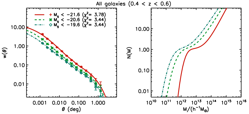
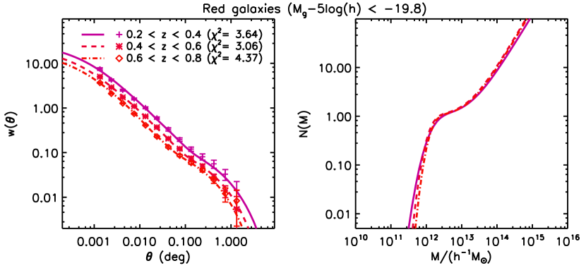
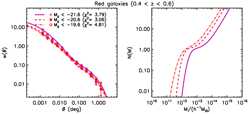
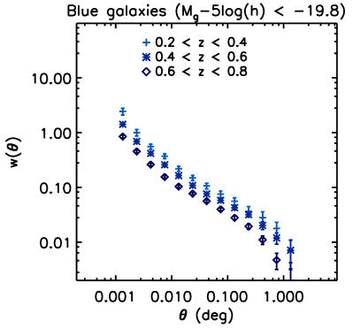
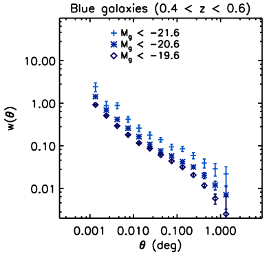
Our measurements are presented in Figure 9, 10 and 11 for the full, red and blue samples, respectively. For clarity, we show three samples selected with the same luminosity threshold (Mg5logh<19.8subscript𝑀𝑔519.8M_{g}-5\log h<-19.8) and three samples covering the same redshift range (0.4<z<0.60.4𝑧0.60.4<z<0.6). At the same luminosity and redshift, red samples are more clustered on small scales than the full sample, and blue galaxies are the least clustered. At a constant luminosity threshold, w(θ)𝑤𝜃w(\theta) increases with redshift for the full, red and blue samples.
Refer to caption
Refer to caption
Figure 9: w(θ)𝑤𝜃w(\theta) measurements (left) with their best fit models for all galaxies, and the resulting galaxy occupation function (right) with respect to halo mass. We illustrate the redshift evolution (top) in the luminosity threshold Mg5logh<19.8subscript𝑀𝑔519.8M_{g}-5\log h<-19.8, and the luminosity dependence (bottom) in the redshift range 0.4<z<0.60.4𝑧0.60.4<z<0.6.
Refer to caption
Refer to caption
Figure 10: w(θ)𝑤𝜃w(\theta) measurements (left) with their best fit models for red galaxies, and the resulting galaxy occupation function (right) with respect to halo mass. We illustrate the redshift evolution (top) in the luminosity threshold Mg5logh<19.8subscript𝑀𝑔519.8M_{g}-5\log h<-19.8, and the luminosity dependence (bottom) in the redshift range 0.4<z<0.60.4𝑧0.60.4<z<0.6.
Refer to caption
Refer to caption
Figure 11: w(θ)𝑤𝜃w(\theta) measurements for blue galaxies. We illustrate the redshift evolution (left) at the luminosity threshold Mg5logh<19.8subscript𝑀𝑔519.8M_{g}-5\log h<-19.8, and the luminosity dependence (right) in the redshift range 0.4<z<0.60.4𝑧0.60.4<z<0.6.

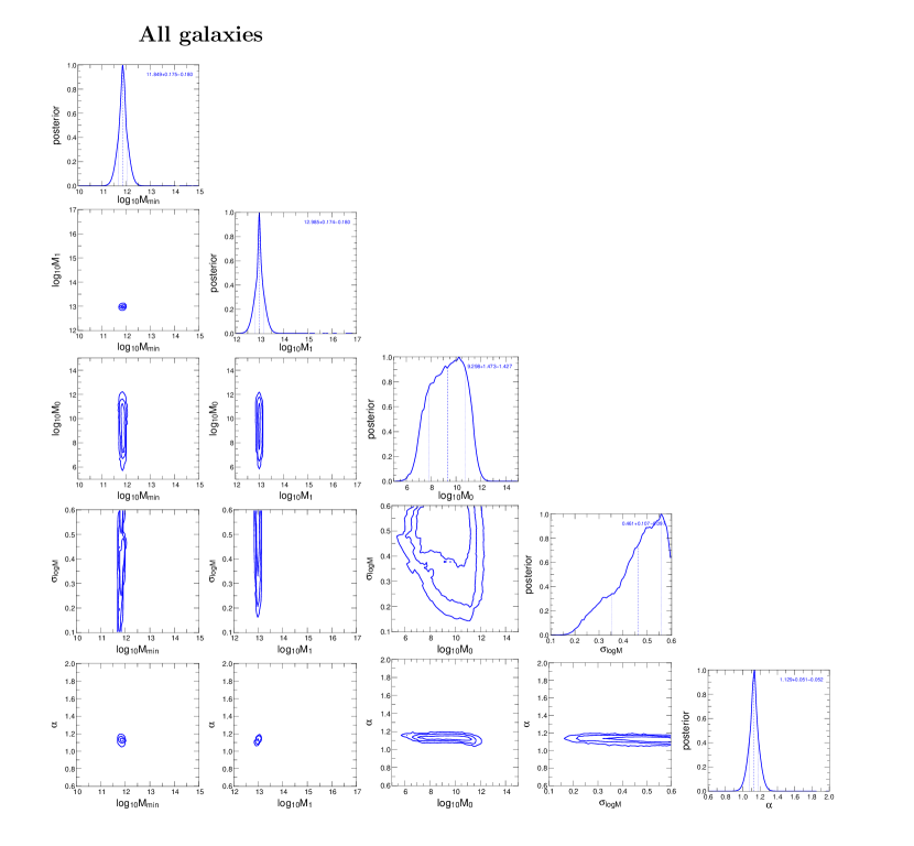
On the left panels of Figs. 9 and 10, we plot our best fit w(θ)𝑤𝜃w(\theta) models. Model parameters and deduced quantities are shown in Tables 1 (full) and 2 (red). An example of sample distributions of best-fitting HOD parameters is given in Fig. 20. Since the halo model aims to reproduce the clustering in threshold samples as a sum of contributions from central and satellite galaxies, both types of galaxy must be present. We presume that in general, central galaxies are brighter than their satellites, so that the latter assumption is valid for full samples selected by luminosity threshold. Also, we assume that red satellites are systematically associated with a (brighter) red central galaxy. On the contrary blue satellites may belong to a red central galaxy. For this reason, we defer fitting our model to our pure blue samples. We plan to address the blue population in a future work, perhaps considering separate halo occupation functions for both red and blue populations (Simon et al., 2009; Skibba & Sheth, 2009).

In most cases, we find a good agreement between the data and our model, with χ2/dofsuperscript𝜒2dof\chi^{2}/\rm dof from 1.77 to 10.21 for full samples and from 1.20 to 6.21 for red samples. We report a few large χ2superscript𝜒2\chi^{2} values in some full samples, mostly at high redshift and for bright luminosity thresholds, where the galaxy number density is small. We suspect systematic photometric redshift errors to be responsible for an underestimated clustering signal and systematic errors in the galaxy number density estimates (see Sec 3.2). Perplexity (see Sect. 4.3) is larger than 0.6 for most samples, indicating that our model accurately describes the observations.

5.2 Halo model fitting

In the right panels of Figs. 9 and 10 we show our best fit N(M)𝑁𝑀N(M), the halo occupation function. First, we note that at a given redshift interval, Mminsubscript𝑀minM_{\rm min}, the average mass for which 50% of haloes contain one galaxy increases with luminosity. Secondly, we note that the evolution in N(M)𝑁𝑀N(M) with redshift at a fixed luminosity is less pronounced than the evolution with luminosity at a fixed redshift, whereas the amplitude of w(θ)𝑤𝜃w(\theta) significantly decreases with redshift.

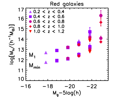
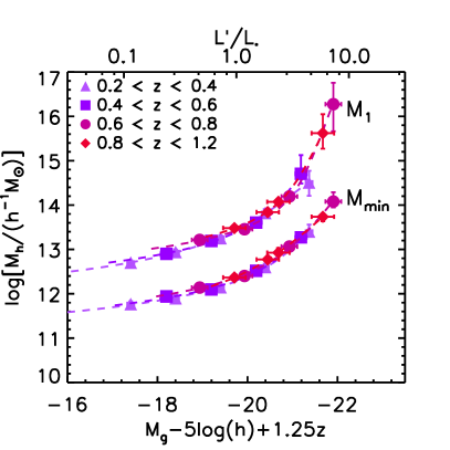
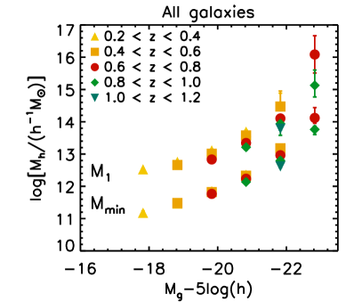
Halo masses M1subscript𝑀1M_{1} and Mminsubscript𝑀minM_{\rm min} are tightly constrained, whereas M0subscript𝑀0M_{0}, σlogMsubscript𝜎log𝑀\sigma_{{\rm log}M} and α𝛼\alpha are poorly constrained. Mminsubscript𝑀minM_{\rm min} and M1subscript𝑀1M_{1} measurements are displayed in the top panels of Fig. 12 with respect to luminosity threshold (Mgsubscript𝑀𝑔M_{g}). For every sample, halo masses increase with luminosity. Mminsubscript𝑀minM_{\rm min} covers the range 1011superscript101110^{11} to 1014h1Msuperscript1014superscript1subscript𝑀10^{14}h^{-1}M_{\sun}. M1subscript𝑀1M_{1} is significantly larger than Mminsubscript𝑀minM_{\rm min}, ranging from 1012.5superscript1012.510^{12.5} to 1016h1Msuperscript1016superscript1subscript𝑀10^{16}h^{-1}M_{\sun}. These trends are consistent with those found in both the local (Zehavi et al., 2010, 2005) and distant Universe studies (Zheng et al., 2007; Abbas et al., 2010). At high luminosity thresholds, where the number of objects is small, error bars on our best-fitting parameters are correspondingly larger. This trend is especially pronounced for α𝛼\alpha, where the small number of satellites in high mass haloes makes it difficult to constrain this parameter. However, we note α𝛼\alpha increases with luminosity threshold, suggesting that for massive haloes, bright galaxies will be more numerous than faint ones. σlogMsubscript𝜎log𝑀\sigma_{{\rm log}M} remains relatively stable for red galaxies (0.3similar-toabsent0.3\sim 0.3), as also seen in other data sets and numerical simulations. For the full sample, values are slightly larger (up to 0.5similar-toabsent0.5\sim 0.5 in some cases). Our fitted σlogMsubscript𝜎𝑀\sigma_{\log M} values are slightly larger than previous works. We also made fits where values σlogM>0.6subscript𝜎𝑀0.6\sigma_{\log M}>0.6 were allowed, and in some cases large values (>1.0absent1.0>1.0) were found. We therefore decided to impose the restriction that σlogM<0.6subscript𝜎𝑀0.6\sigma_{\log M}<0.6. Sample incompleteness (due to errors in the photometric redshifts), leading to missing central galaxies, could explain such high σlogMsubscript𝜎𝑀\sigma_{\log M} values.

At constant luminosity threshold, in both red and full samples, M1subscript𝑀1M_{1} and Mminsubscript𝑀minM_{\rm min} decrease with increasing redshift. This effect is partially due to a selection effect caused by the dimming and reddening of stellar populations with time; for a constant luminosity cut one selects less and less massive galaxies at higher redshifts. We will return to this measurement in Sect. 6 where we attempt to separate this passive stellar evolution effect from the intrinsic stellar-to-halo mass evolution.

At faint luminosities, Mminsubscript𝑀minM_{\rm min} values are higher for red galaxies than for full samples. As we explained previously, one assumption of our model is that our red threshold samples have luminous red central galaxies. On the other hand, it is also possible, especially for fainter samples, that blue satellite galaxies inhabit haloes with red central galaxies. In such a case for the faint red galaxy sample, a red central galaxy will be seen “alone” in a more massive halo. This would also increase the halo mass estimate found for red central galaxies as compared to those in the full sample.

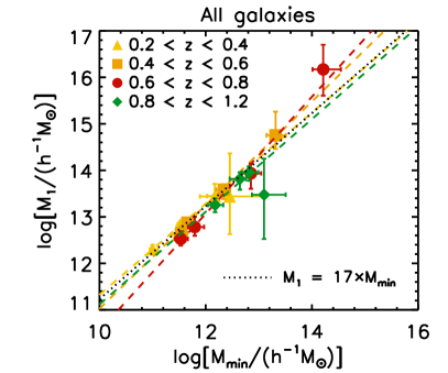
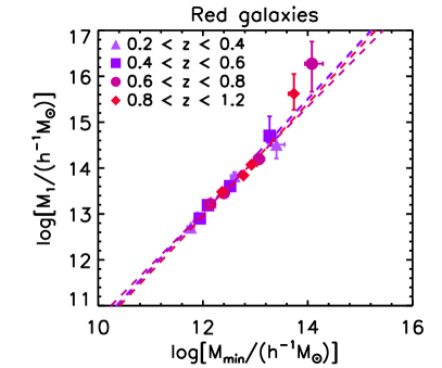
The bottom panels of Fig. 12 show M1subscript𝑀1M_{1} with respect to Mminsubscript𝑀minM_{\rm min} for full and red samples. The parameters are strongly correlated and we fitted a power law (dashed line) in each redshift bin. For the full sample, we compare our results with a linear relation, M1=17×Mminsubscript𝑀117subscript𝑀minM_{1}=17\times M_{\rm min} (dotted line), based on the coefficient observed in the SDSS (z0.1similar-to𝑧0.1z\sim 0.1) by Zehavi et al. (2010). Our results agree with them in the lowest redshift bin, z0.3similar-to𝑧0.3z\sim 0.3, but depart from this value at higher redshift.

We find that although M1/Mminsubscript𝑀1subscript𝑀minM_{1}/M_{\rm min} relation does not vary significantly with luminosity threshold it does show some indications of evolution with redshift. We note that M1/Mminsubscript𝑀1subscript𝑀minM_{1}/M_{\rm min} decreases with redshift for Mmin1013h1Mless-than-or-similar-tosubscript𝑀minsuperscript1013superscript1subscript𝑀direct-productM_{\rm min}\lesssim 10^{13}h^{-1}M_{\odot} and increases with redshift at higher mass. For red galaxies, M1subscript𝑀1M_{1} is no longer proportional to Mminsubscript𝑀minM_{\rm min} but follows a power law. For Mmin1012h1Msimilar-tosubscript𝑀minsuperscript1012superscript1subscript𝑀direct-productM_{\rm min}\sim 10^{12}h^{-1}M_{\odot}, the ratio M1/Mminsubscript𝑀1subscript𝑀minM_{1}/M_{\rm min} is 12similar-toabsent12\sim 12 (as compared to 10similar-toabsent10\sim 10 for luminous red galaxies found by Zheng et al., 2009) and shows a much smaller redshift evolution over the entire mass range.
Refer to caption
Refer to caption
Refer to caption
Refer to caption
Figure 12: Top panels: halo mass estimates Mminsubscript𝑀minM_{\rm min} and M1subscript𝑀1M_{1} for all (left) and red (right) galaxy samples as function of luminosity threshold (Mgsubscript𝑀𝑔M_{g}). Bottom panels: M1subscript𝑀1M_{\rm 1} versus Mminsubscript𝑀minM_{\rm min} in different redshift bins. The dotted lines represent a linear relation and the dashed lines are a power-law fit to M1subscript𝑀1M_{1} versus Mminsubscript𝑀minM_{\rm min} in each redshift bin.
Refer to caption
Refer to caption
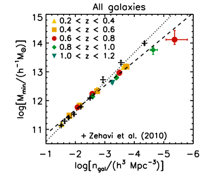
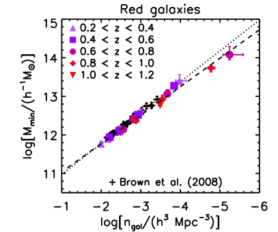
Figure 13: Mminsubscript𝑀minM_{\rm min} as a function of galaxy number density for all (left) and red (right) galaxies. The dashed line in each panel represents a power law fit to the data, and the dotted line represents a power law fit to the results given in Brown et al. (2008) (red galaxies) and in the SDSS by Zehavi et al. (2010) (all galaxies). We converted M200subscript𝑀200M_{200} halo masses to virial masses Mvirsubscript𝑀𝑣𝑖𝑟M_{vir} when necessary.

Figure 13 shows the relationship between Mminsubscript𝑀minM_{\rm min} and the galaxy number density ngalsubscript𝑛galn_{\rm gal} for red and full samples. As one would expect, progressively rarer objects are found in more massive haloes. We do not detect a significant evolution of the slope of our Mminsubscript𝑀minM_{\rm min} versus ngalsubscript𝑛galn_{\rm gal} relationship with redshift. For red galaxies, we overplot the measurements from Brown et al. (2008) with which we are in excellent agreement, even though it covers a much smaller area, For the full galaxy sample we compare with SDSS measurements (Zehavi et al., 2010). The agreement is good at high surface densities; however we note a departure for low density samples. This difference suggests that at constant density, galaxies tend to reside in more massive haloes at low redshift (z0similar-to𝑧0z\sim 0) than at higher redshift (z>0.6𝑧0.6z>0.6). Part of this difference could be caused by systematic photometric redshift errors. As we discussed in Sec 3.2, bright samples may be contaminated by fainter objects, and the combined effect of higher density and lower clustering signal will result in reducing Mminsubscript𝑀minM_{\rm min}. In the most pessimistic case outlined in Sec 3.2, where the density estimate would be overestimated by a factor 3, logMminsubscript𝑀min\log M_{\rm min} would be biased low by a few sigmas (up to 0.5similar-toabsent0.5\sim 0.5).

The relationship between Mminsubscript𝑀minM_{\rm min} and ngalsubscript𝑛galn_{\rm gal} can be well approximated by a power law and we fitted galaxy samples at all redshifts simultaneously. We found:

Mminall=1010.0×[ngalall/(h3Mpc3)]0.84h1M,superscriptsubscript𝑀minallsuperscript1010.0superscriptdelimited-[]superscriptsubscript𝑛galallsuperscript3superscriptMpc30.84superscript1subscript𝑀M_{\rm min}^{\rm all}=10^{10.0}\times[n_{\rm gal}^{\rm all}/(h^{3}\,{\rm Mpc^{-3}})]^{-0.84}\,h^{-1}\,M_{\sun}\,, (22)

for all galaxies and

Mminred=1010.3×[ngalred/(h3Mpc3)]0.74h1M,superscriptsubscript𝑀minredsuperscript1010.3superscriptdelimited-[]superscriptsubscript𝑛galredsuperscript3superscriptMpc30.74superscript1subscript𝑀M_{\rm min}^{\rm red}=10^{10.3}\times[n_{\rm gal}^{\rm red}/(h^{3}\,{\rm Mpc^{-3}})]^{-0.74}\,h^{-1}\,M_{\sun}\,, (23)

for red galaxies.

6 Discussion

The key issue we would like to address is to understand how galaxy formation and evolution depend on the properties of the underlying dark matter haloes. Ideally, to relate halo masses to their stellar content, one would select our samples by stellar mass. However, stellar mass estimates computed from our five-band optical data alone would suffer from large uncertainties. Keeping this limitation in mind, we adopt an intermediate approach where we determine an empirical relation to convert the observed luminosity threshold of each sample to an approximately mass-selected sample using a reference sample with accurate stellar masses. This method allows to transform luminosities into masses and provides an estimate of the likely errors in such a transformation.

6.1 Transforming to stellar mass threshold samples

As a consequence of passive stellar evolution, the characteristic rest-frame Mgsubscript𝑀𝑔M_{g}-band luminosity of a given galaxy type evolves significantly over the redshift range 0.2<z<1.20.2𝑧1.20.2<z<1.2 (Ilbert et al., 2005; Zucca et al., 2006; Faber et al., 2007).

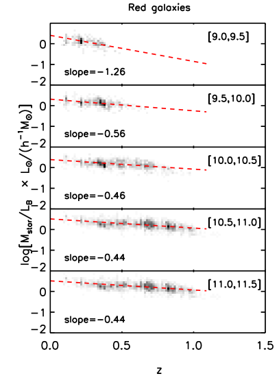
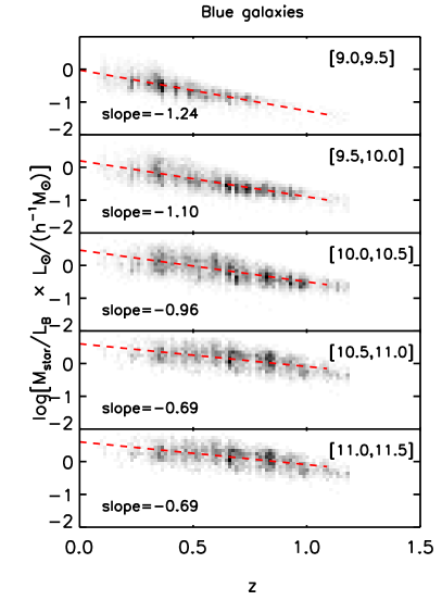
In order to account for these effects, we have established a simple approximation to relate stellar mass and luminosity based on COSMOS 30-band photometry (Ilbert et al., 2010). We used the COSMOS Blimit-from𝐵B-band luminosities in order to be as close as possible to our Mgsubscript𝑀𝑔M_{g}-band selected samples. Red galaxies are selected as M(NUV)MR>3.5𝑀𝑁𝑈𝑉subscript𝑀𝑅3.5M(NUV)-M_{R}>3.5 and blue galaxies as M(NUV)MR3.5𝑀𝑁𝑈𝑉subscript𝑀𝑅3.5M(NUV)-M_{R}\leq 3.5. We then fit the stellar mass-to-luminosity ratio with power-law functions as function of redshift between z=0𝑧0z=0 and z=1.5𝑧1.5z=1.5 for five stellar mass bins from 109.0superscript109.010^{9.0} to 1011.5superscript1011.510^{11.5}. These results are displayed in Fig. 14.

Due to the ageing of stellar populations, the average stellar mass-to-light ratio increases with time. For red galaxies, the slope depends weakly on stellar mass at intermediate masses (109.51011.5h1Msuperscript109.5superscript1011.5superscript1subscript𝑀10^{9.5}-10^{11.5}h^{-1}M_{\sun}) and ranges from 0.560.56-0.56 to 0.440.44-0.44. The slope is steepest in the lowest mass bin, but the number of objects in this bin is small. Based on these results we adopt the following relationship for the red galaxy population:

log(MstarLB)red=log(MstarLB)red,z=0(0.5±0.1)z,\log\left(\frac{M_{\rm star}}{L_{B}}\right)_{\rm red}=\log\left(\frac{M_{\rm star}}{L_{B}}\right)_{{\rm red,}z=0}-(0.5\pm 0.1)z\,, (24)

where the 0.10.10.1 error accounts for the scatter between mass bins. This evolution is consistent with the luminosity function evolution measured for red galaxies in the DEEP2 and COMBO17 surveys (Faber et al., 2007; Willmer et al., 2006), where the characteristic absolute magnitude MBsuperscriptsubscript𝑀𝐵M_{B}^{\ast} decreases by about 1.2–1.3 mag per unit redshift (MB2.5logLBproportional-tosubscript𝑀𝐵2.5subscript𝐿𝐵M_{B}\propto-2.5\log L_{B}).

For the blue sample, the evolution in redshift is more pronounced than for the red sample, as also seen in DEEP2 (Willmer et al., 2006) and VVDS (Zucca et al., 2006). Unfortunately, in this case, the slope depends on stellar mass, ranging from 0.690.69-0.69 to 1.101.10-1.10 in the mass range [109.5,1011.5]superscript109.5superscript1011.5[10^{9.5},10^{11.5}], and has a larger scatter. The full sample is dominated by blue galaxies at faint luminosities but by red galaxies at bright luminosity (see Fig. 3). Therefore a simple relation between luminosity and stellar mass valid for all luminosities cannot be obtained. For the full sample we choose to apply the same correction as for the red sample. As blue galaxies evolve more rapidly than red ones such a correction underestimates the expected evolution of the full samples at faint luminosity and therefore cannot be used to construct stellar-mass selected samples. In the following sections, we discuss how our results depend on this correction.

In the following sections we use these expressions to calculate “corrected” luminosities, denoted as Lsuperscript𝐿L^{\prime}. Note that these corrections are equivalent to shifting observed galaxy luminosities to redshift z=0𝑧0z=0. Our results are displayed as a function of relative luminosity threshold L/Lsuperscript𝐿subscript𝐿L^{\prime}/L_{\ast}, where Lsubscript𝐿L_{\ast} corresponds to Mg5logh=19.81subscriptsuperscript𝑀𝑔519.81M^{\ast}_{g}-5\log h=-19.81 and 19.7519.75-19.75 for the full and red samples, respectively, measured in the local Universe (Faber et al., 2007, and references therein). It is also worth mentioning that if galaxies would experience a pure passive luminosity evolution with cosmic time, this would result in constant HOD parameters for a given L/Lsuperscript𝐿subscript𝐿L^{\prime}/L_{\ast} as function of redshift. However, deduced parameters (galaxy bias, mean halo mass and satellite fraction) are expected to vary due to the evolving halo mass function and halo bias (see Eqs. 1317).

Refer to caption
Refer to caption
Figure 14: Stellar mass-to-luminosity relations for red (left) and blue (right) galaxies, as a function of stellar mass and redshift as measured in the COSMOS survey (Ilbert et al., 2009). Each panel shows a separate slice in stellar mass. Samples are fitted with a power law (dashed line).

6.2 The stellar-to-halo mass relationship
Refer to caption
Refer to caption
Refer to caption
Refer to caption
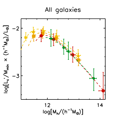
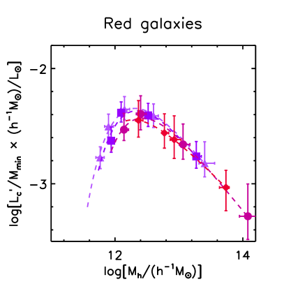
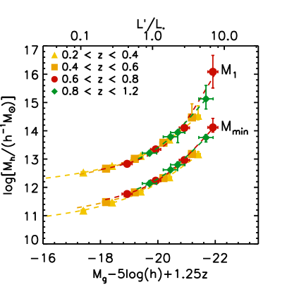
Figure 15: Left panels: halo mass estimates Mminsubscript𝑀minM_{\rm min} and M1subscript𝑀1M_{1} for all (top) and red (bottom) galaxy samples, as function of luminosity threshold, corrected for passive redshift evolution to approximate stellar mass selected samples. The dashed lines correspond to Eq. 25. Right panels: light-to-halo mass ratios Lc/Mminsubscriptsuperscript𝐿csubscript𝑀minL^{\prime}_{\rm c}/M_{\rm min} (Eq. 26 with identical parameters as those fitted with Eq. 25) as function of halo mass.

In our model, Mminsubscript𝑀minM_{\rm min} represents the hosting halo mass for central galaxies whose median luminosity equals the luminosity threshold of the sample (see Sect. 4.1). The ratio L/Mminsuperscript𝐿subscript𝑀minL^{\prime}/M_{\rm min} is therefore the ratio of luminosity to dark matter mass for central galaxies. Zehavi et al. (2010) showed that the relation between central galaxy luminosity Lcsubscriptsuperscript𝐿cL^{\prime}_{\rm c} (corresponding to our Lsuperscript𝐿L^{\prime}) and the halo mass could be approximated by:

LcL=A(MhMt)αMexp(MtMh+1),subscriptsuperscript𝐿csubscript𝐿𝐴superscriptsubscript𝑀hsubscript𝑀tsubscript𝛼𝑀subscript𝑀tsubscript𝑀h1\frac{L^{\prime}_{\rm c}}{L_{\ast}}=A\left(\frac{M_{\rm h}}{M_{\rm t}}\right)^{\alpha_{M}}\exp\left(-\frac{M_{\rm t}}{M_{\rm h}}+1\right)\,, (25)

where A, αMsubscript𝛼𝑀\alpha_{M} and Mtsubscript𝑀tM_{\rm t} are free parameters and Mhsubscript𝑀hM_{\rm h} represents Mminsubscript𝑀minM_{\rm min} or M1subscript𝑀1M_{1}.

This expression encapsulates the idea that there exists a “transition halo mass” (Mtsimilar-toabsentsubscript𝑀𝑡\sim\leavevmode\nobreak\ M_{t}) where the ratio of central galaxy luminosity to dark matter halo mass reaches a maximum. This transition mass represents the halo mass for which baryons have been most efficiently converted into stars until the time of observation, resulting from past and on-going star formation over cosmic history.

We fit Eq. 25 for full and red samples for each redshift slice. For our two highest redshift bins where the number of points are less than the number of free parameters, we perform a simultaneous fit over both redshift bins. Results are plotted in Fig. 15 and best-fitting parameters given in Table 9.

In our lowest redshift bin (0.2<z<0.40.2𝑧0.40.2<z<0.4), our full sample has best-fitting parameters slightly different than in the SDSS (Zheng et al., 2007; Zehavi et al., 2010), A=0.20±0.01𝐴plus-or-minus0.200.01A=0.20\pm 0.01 (compared to 0.32) and Mt=2.24±0.1×10¹¹h1Msubscript𝑀tplus-or-minus2.240.1superscript1011superscript1subscript𝑀M_{\rm t}=2.24\pm 0.1\times 10^{11}h^{-1}M_{\sun} (compared to 3.08×10113.08superscript10113.08\times 10^{11}). We note that the difference is likely due to the different selection (Mrsubscript𝑀𝑟M_{r} in the SDSS). At high luminosities, the difference with their relation increases. For a given luminosity, we find lower halo masses, LcM0.5±0.01proportional-tosubscript𝐿csuperscript𝑀plus-or-minus0.50.01L_{\rm c}\propto M^{0.5\pm 0.01}, compared to LcM0.260.28proportional-tosubscript𝐿csuperscript𝑀0.260.28L_{\rm c}\propto M^{0.26-0.28}, which follows the trends observed in Fig. 13, and might be due to contaminated samples at low density. In the red sample, we measure LcM0.31±0.16proportional-tosubscript𝐿csuperscript𝑀plus-or-minus0.310.16L_{\rm c}\propto M^{0.31\pm 0.16}, whereas Zheng et al. (2009) found LcM0.5proportional-tosubscript𝐿csuperscript𝑀0.5L_{\rm c}\propto M^{0.5} for luminous red galaxies in the SDSS. Both Mminsubscript𝑀minM_{\rm min} and M1subscript𝑀1M_{1} increase with redshift for the full sample. The dependence with redshift is weak for red galaxies, although we detect a slight increase in the very highest redshift bins.

For the full sample we assumed a correction based on the evolution of the stellar mass-to-luminosity ratio of red galaxies (Eq. 24). As the characteristic luminosity of blue galaxies evolves more rapidly than red ones and as the faint sample is dominated by blue galaxies a legitimate concern is the dependence of our results on our corrections to stellar mass. Several corrections assuming the blue galaxy luminosity evolution (using slopes given in Fig. 14) were tested. If a larger correction is applied, M1subscript𝑀1M_{1} and Mminsubscript𝑀minM_{\rm min} show a similar but more pronounced trend. For this reason we conclude that the increase of halo mass parameters with redshift for the full sample is a robust result (although the exact amount of evolution observed depends on the correction we apply).

6.3 Redshift evolution of the SHMR and comparison with literature values
Refer to caption
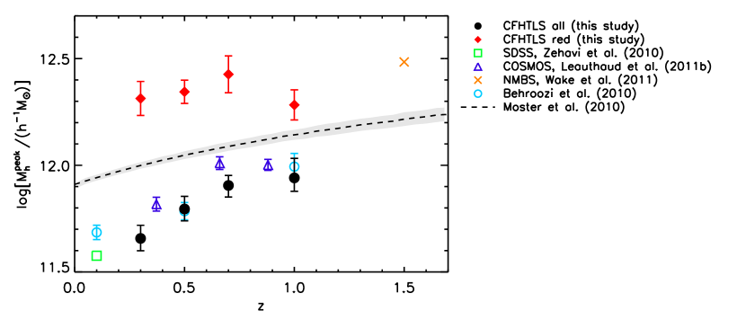
Figure 16: Position of the peak Mhpeaksubscriptsuperscript𝑀peakhM^{\rm peak}_{\rm h} corresponding to max(Lc/Mmin)subscriptsuperscript𝐿csubscript𝑀min\max(L^{\prime}_{\rm c}/M_{\rm min}) for the full (filled circles) and red (filled diamonds) samples as function of redshift. Error bars are derived from the nearest data point to the peak. We compare our results with measurements in SDSS (Zehavi et al., 2010), in COSMOS (Leauthaud et al., 2011b) and in the NEWFIRM Medium Band Survey (NMBS, Wake et al., 2011). We convert M200subscript𝑀200M_{200} halo masses (corresponding to a sphere with overdensity 200 times the background density) into virial masses Mvirsubscript𝑀virM_{\rm vir} (our definition) using the method described in Appendix C of Hu & Kravtsov (2003). We also display numerical predictions based on abundance-matching method from Behroozi et al. (2010) and Moster et al. (2010), where the shaded region shows the 1σ𝜎-\sigma uncertainty.

To study the redshift evolution of the stellar-to-halo mass ratio, we consider the relationship between corrected galaxy luminosity and the host halo mass from Eq. 25:

LcMh=ALMt(MhMt)αM1exp(MtMh+1),subscriptsuperscript𝐿csubscript𝑀h𝐴subscript𝐿subscript𝑀tsuperscriptsubscript𝑀hsubscript𝑀tsubscript𝛼𝑀1subscript𝑀tsubscript𝑀h1\frac{L^{\prime}_{\rm c}}{M_{\rm h}}=A\,\frac{L_{\ast}}{M_{\rm t}}\left(\frac{M_{\rm h}}{M_{\rm t}}\right)^{\alpha_{M}-1}\exp\left(-\frac{M_{\rm t}}{M_{\rm h}}+1\right)\,, (26)

where the maximum is located at:

Mhpeak=Mt1αM.subscriptsuperscript𝑀peakhsubscript𝑀t1subscript𝛼𝑀M^{\rm peak}_{\rm h}=\frac{M_{\rm t}}{1-\alpha_{M}}\,. (27)

The right panels of Fig. 15 show the Lc/Mminsubscriptsuperscript𝐿𝑐subscript𝑀minL^{\prime}_{c}/M_{\rm min} relation for full and red samples as function of halo mass fitted by Eq. 25. Best fitting parameters are listed in Table 9. For less massive haloes, the relative stellar mass content increases with halo mass and reaches a maximum around Mmin1012h1Msimilar-tosubscript𝑀minsuperscript1012superscript1subscript𝑀M_{\rm min}\sim 10^{12}h^{-1}M_{\sun}. In more massive haloes, the stellar-to-halo mass ratio sharply decreases. Our measurements are consistent with recent observations measuring the stellar-to-halo mass ratio as function of halo mass (Mandelbaum et al., 2006; Zheng et al., 2007; Foucaud et al., 2010; Zehavi et al., 2010; More et al., 2011; Wake et al., 2011; Leauthaud et al., 2011b), and “abundance-matching” techniques based on N𝑁N-body simulations (Conroy & Wechsler, 2009; Moster et al., 2010; Behroozi et al., 2010). Similar trends are found in semi-analytic simulations (see, for e.g., Somerville et al., 2008), in which physical processes (such as supernovae and AGN feedback) preventing gas from cooling and quenching star formation must be taken into account to match observations.

Our measured peak values Mhpeaksubscriptsuperscript𝑀peakhM^{\rm peak}_{\rm h} (Eq. 27, with error bars from the nearest data points) are plotted as a function of redshift in Fig. 16. Comparing to literature measurements at lower redshifts, the peak stellar-to-halo mass relation is Mhpeak=4.54×10¹¹h1Msubscriptsuperscript𝑀peakh4.54superscript1011superscript1subscript𝑀direct-productM^{\rm peak}_{\rm h}=4.54\times 10^{11}h^{-1}M_{\odot}, similar to the local Universe value (4.2×10¹¹h1Mabsent4.2superscript1011superscript1subscript𝑀direct-product\approx 4.2\times 10^{11}h^{-1}M_{\odot}, Zehavi et al., 2010). For our full sample, the peak location gradually increases with redshift.

At higher redshifts, we compare our measurements with those of Moster et al. (2010) and Behroozi et al. (2010). These authors derived the stellar-to-halo mass relation using an abundance-matching technique, linking dark matter halo mass functions from N𝑁N-body simulations with observed galaxy stellar mass functions. Moster et al. (2010) estimate the redshift evolution of the stellar-to-halo mass ratio (their Table 7) and from this we derived analytically the position of the peak, as well as associated errors. Values from Behroozi et al. (2010) at redshift 0.1, 0.5 and 1.0 were supplied to us (P. Behroozi, private communication). Both Moster et al. and Behroozi et al.’s measurements are based primarily on galaxy stellar mass measurements covering relatively small areas (a few hundred square arcminutes). Our full sample is in excellent agreement with Behroozi et al. but differs significantly from Moster et al., although in both cases the two data sets show the same general trend: Mhpeaksubscriptsuperscript𝑀peakhM^{\rm peak}_{\rm h} shifts gradually towards higher halo masses at higher redshift. The Moster et al. points do not seem to agree very well with most observations and moreover overestimate the position of the peak at low redshift.

Measurements in the COSMOS field are also shown (Leauthaud et al., 2011b); their points are in general larger than most measurements, with the exception of Moster et al.. It has already been noted that there are several rich structures in the COSMOS field (McCracken et al., 2007; Meneux et al., 2009; de la Torre et al., 2010) which lead to higher correlation functions, especially at z0.8similar-to𝑧0.8z\sim 0.8; cosmic variance could perhaps be the origin of this discrepancy.

For red galaxies, the peak is at larger halo masses, Mhpeak=20.6×10¹¹h1Msubscriptsuperscript𝑀peakh20.6superscript1011superscript1subscript𝑀direct-productM^{\rm peak}_{\rm h}=20.6\times 10^{11}h^{-1}M_{\odot}. This is not surprising as Mminsubscript𝑀minM_{\rm min} is larger for red galaxies at faint luminosities. The red galaxy peak position undergoes only little evolution to z1similar-to𝑧1z\sim 1. Our intermediate-redshift red galaxy points are consistent with higher redshift measurements (Wake et al., 2011); these authors used a near-infrared survey to select galaxies by stellar mass, and we would expect their selection to be dominated by red galaxies.

The results presented here represent the first time a single data set covering a statistically significant area has been used to derive the evolution of the peak position as a function of redshift and galaxy type in a self-consistent manner. The peak position, Mhpeaksubscriptsuperscript𝑀peakhM^{\rm peak}_{\rm h}, can be interpreted as representing the halo mass at which the stellar mass content is most efficiently accumulated in haloes, either by star formation or merger processes. The movement of this peak towards higher halo masses at higher redshifts is consistent with a picture in which the sites of efficient stellar mass growth migrate from low-mass to high-mass haloes at higher redshift. This “anti-hierarchical” evolution, frequently referred to as “halo downsizing”, resembles closely the scenario first sketched by Cowie et al. (1996), in which the maximum luminosity of galaxies undergoing star-formation declines steadily to the current day. Conversely, the fact that we observe constant transition masses for the red population suggests that the stellar-to-halo mass ratio does not significantly evolve in haloes with mass 1012h1Msimilar-toabsentsuperscript1012superscript1subscript𝑀direct-product\sim 10^{12}h^{-1}M_{\odot} and supports observations that intermediate-mass red galaxies have experienced no significant stellar mass growth by star formation since z1.2similar-to𝑧1.2z\sim 1.2.

We tried several corrections to convert to stellar mass thresholds based on the slope measured for blue galaxy evolution (see Fig. 14), and we found that the peak luminosity depends only weakly on these corrections. Only the highest-redshift point changes by around one sigma if we apply the extreme “blue galaxy” correction to our full sample. For this reason we conclude that the increase of Mhpeaksubscriptsuperscript𝑀peakhM^{\rm peak}_{\rm h} with redshift for the full sample is a robust result.

6.4 Redshift evolution of halo satellite fraction

The fraction of galaxies which are satellites in a given dark matter halo is a sensitive probe of the past evolutionary history of the halo which may be modified by processes such as major mergers (which can decrease the satellite fraction with time) or environmental effects which operate primarily to reduce the number of satellites, such as, but not limited to, the restriction of gas supply or “strangulation” (Larson et al., 1980) or ram-pressure stripping (Gunn & Gott, 1972). Satellite galaxies may also merge with their central galaxy. Observational evidence based on pair fraction measurements and theoretical studies using numerical simulations now shows that mergers seem to play a significant (although not dominant) role in the evolution of massive galaxies since z1similar-to𝑧1z\sim 1 (White et al., 2007; Wang & Jing, 2010; van Dokkum et al., 2010; Robaina et al., 2010; Zehavi et al., 2011). Our objective in this section is to see if measurements of the satellite fraction can provide new insights into the evolutionary history of haloes.

The left panels of Figure 17 show the satellite fraction fssubscript𝑓sf_{\rm s}, computed using Eq. 17. As before, each sample is converted to an approximately mass-limited sample by “correcting” for passive luminosity evolution (see Sect. 6.1).
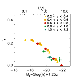
Refer to caption Refer to caption Refer to caption
Figure 17: Satellite fractions as function of luminosity and redshift, for all and red samples (top and bottom panels). The left panels show the measured satellite fraction as function of corrected luminosity. Dashed lines in the middle panels show satellite fractions extrapolated in redshift, based on our HOD parameters measured in the redshift range 0.4<z<0.60.4𝑧0.60.4<z<0.6. We compare our results with the literature for all galaxies at z=0.1𝑧0.1z=0.1 and z=1.0𝑧1.0z=1.0 (top, Zheng et al., 2007) and with galaxy-galaxy lensing estimates at z=0.1𝑧0.1z=0.1 (bottom, Mandelbaum et al., 2006) for red galaxies. In the right panels we provide values extrapolated in redshift for several L/Lsuperscript𝐿subscript𝐿L^{\prime}/L_{\ast} ratios.

At all redshifts, as the luminosity threshold increases, corresponding to higher mass thresholds, the satellite fractions become progressively smaller. The similarity between the full and red samples is simply a consequence of the dominance of red galaxies at bright luminosity thresholds.

At fainter luminosity thresholds, the satellite fraction rises and eventually reaches a plateau. This effect can be understood by considering both the halo mass function and the halo occupation function: the increase of the latter with decreasing luminosity threshold (see Fig. 8) is rapidly compensated by a sharp decrease in massive halo number density, so that faint galaxies are preferentially central galaxies in smaller haloes rather than being satellites in more massive haloes.

We compare our results with satellite fractions found in SDSS (z0.1similar-to𝑧0.1z\sim 0.1) and DEEP2 (z1similar-to𝑧1z\sim 1). To explore a complete range in redshift and luminosity, we extrapolate our best-fitting HOD parameters measured in the redshift range 0.4<z<0.60.4𝑧0.60.4<z<0.6; that is, at a given luminosity, we keep the HOD parameters fixed and compute Eq. 17 at different redshifts. The choice for this intermediate redshift range is motivated by the fact that it contains the most robust photometric redshift estimates and our measured points span a large range in luminosity. Each HOD parameter set is constructed from Mminsubscript𝑀minM_{\rm min} and M1subscript𝑀1M_{1} interpolated in luminosity using Eq. 25 with best-fitting parameters given in Table 9. For red galaxies, M0subscript𝑀0M_{0} is set to Mmin/100subscript𝑀min100M_{\rm min}/100, σlogMsubscript𝜎𝑀\sigma_{\log M} is fixed to 0.3 and α=1.1𝛼1.1\alpha=1.1 for L<L𝐿subscript𝐿L<L_{\ast} or α=1.4𝛼1.4\alpha=1.4 otherwise. For all galaxies, M0subscript𝑀0M_{0} is set to Mmin/100subscript𝑀min100M_{\rm min}/100, σlogM=0.4subscript𝜎𝑀0.4\sigma_{\log M}=0.4 and α=1.1𝛼1.1\alpha=1.1 for L<L𝐿subscript𝐿L<L_{\ast}, and σlogM=0.3subscript𝜎𝑀0.3\sigma_{\log M}=0.3 and α=1.3𝛼1.3\alpha=1.3 for brighter luminosity thresholds.

In the middle panels of Fig. 17 we compare our extrapolated satellite fractions for all galaxies (in dashed lines) with results derived from SDSS and DEEP2, using a HOD analysis similar to ours (Zheng et al., 2007). Our satellite fractions are consistent with these measurements at both redshifts, although we slightly over-predict satellite fractions at z0.1similar-to𝑧0.1z\sim 0.1 for samples brighter than 0.5Lsimilar-toabsent0.5subscript𝐿\sim 0.5L_{\ast}. An overall increase of a factor of two is measured between z1similar-to𝑧1z\sim 1 and z0similar-to𝑧0z\sim 0 for samples with L>L𝐿subscript𝐿L>L_{\ast}; we note that this value is lower than the factor of three from z0.5similar-to𝑧0.5z\sim 0.5 to z0similar-to𝑧0z\sim 0 measured in the VVDS (Abbas et al., 2010).

We fit the HOD parameters at each redshift independently. Therefore, our model provides us with “snapshots” of the occupation function at various epochs. If any physical process had played a significant role in reducing the satellite number density between z1similar-to𝑧1z\sim 1 and z0similar-to𝑧0z\sim 0, our fixed-HOD model calibrated at z0.5similar-to𝑧0.5z\sim 0.5 would over-predict the satellite fraction observed in the local Universe and under-predict the satellite fraction at redshift one. The excellent match found for bright luminosity threshold samples shows that our satellite fraction measurements follow closely a redshift-independent HOD. Since a redshift evolution of the merging rate would change the occupation function, we therefore conclude that our measurements imply a constant merging rate since z1similar-to𝑧1z\sim 1, which confirms the constant (albeit minor) role of merging for intermediate-mass galaxies (e.g., Bundy et al., 2009). As outlined by White et al. (2007), if halo merging was not followed by galaxy merging, we would observe an increase of halo masses at constant galaxy density. Instead, no redshift evolution of the Mminsubscript𝑀minM_{\rm min}-ngalsubscript𝑛galn_{\rm gal} relationship (see Fig. 13) supports a scenario with constant galaxy merging with time.

We compare our red satellite fraction with the galaxy-galaxy lensing analysis from SDSS (Mandelbaum et al., 2006). These samples were constructed from luminosity slices, rather than the threshold samples we use here. We then computed the number of satellites per luminosity bin as the difference of satellite fractions between two threshold samples:

fsbin=fsthres2ngalthres2fsthres1ngalthres1ngalthres2ngalthres1.subscriptsuperscript𝑓bin𝑠subscriptsuperscript𝑓thres2𝑠subscriptsuperscript𝑛thres2galsubscriptsuperscript𝑓thres1𝑠subscriptsuperscript𝑛thres1galsubscriptsuperscript𝑛thres2galsubscriptsuperscript𝑛thres1galf^{\rm bin}_{s}=\frac{f^{\rm thres2}_{s}n^{\rm thres2}_{\rm gal}-f^{\rm thres1}_{s}n^{\rm thres1}_{\rm gal}}{n^{\rm thres2}_{\rm gal}-n^{\rm thres1}_{\rm gal}}\,. (28)

As we found for the full galaxy sample, the good agreement supports a non-evolving HOD from z=0.5𝑧0.5z=0.5 to z=0𝑧0z=0.

Finally, in the right panels of Fig. 17, we provide extrapolated satellite fractions as function of redshift for several luminosity thresholds. It is interesting to examine our results in the context of recent results studying the role of satellite galaxies in galaxy formation and evolution (Peng et al., 2010, 2011). These works show measurements from numerical simulations and SDSS group catalogues which indicate that the fraction of satellites at a fixed overdensity is independent of halo mass and redshift. In this context, the growth of the satellite fraction we observe is simply a consequence of average growth in overdensity in rich structures between z1similar-to𝑧1z\sim 1 to z0similar-to𝑧0z\sim 0, reflecting the growing importance of environment at low redshift.

6.5 Galaxy bias

We compute the galaxy bias (Eq. 13) from our best-fitting HOD parameters. We fit the bias measurements as function of luminosity and redshift, adopting a linear relationship (Norberg et al., 2001):

bg(>L)=abias+bbiasLL,annotatedsubscript𝑏𝑔absentsuperscript𝐿subscript𝑎biassubscript𝑏biassuperscript𝐿subscript𝐿b_{g}(>L^{\prime})=a_{\rm bias}+b_{\rm bias}\frac{L^{\prime}}{L_{\ast}}\,, (29)

where Lsuperscript𝐿L^{\prime} represents the corrected luminosity (computed from Eq. 24 for the full and red samples). We fit the two highest redshift bins together (0.8<z<1.00.8𝑧1.00.8<z<1.0, 1.0<z<1.21.0𝑧1.21.0<z<1.2), as only one point is available in the highest one. Results are plotted in Fig. 18 and best-fitting parameters are given in Table 10.
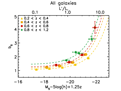
Refer to caption
Refer to caption
Refer to caption
Refer to caption
Figure 18: Galaxy bias as function of luminosity and redshift. Left panels: bias for full and red samples (top and bottom panels) as function of corrected luminosity threshold Lsuperscript𝐿L^{\prime}. The dashed line represents Eq. 29. Right panels: computed bias for several luminosity threshold samples Lsubscriptsuperscript𝐿L^{\prime}_{\ast} as function of redshift. Error bars were derived from the parametric form shown on the left (dashed line), whereas the dotted lines show the bias evolution computed from our model, assuming a redshift-independent HOD parameter set.

This parameterised bias relation reproduces our results best at z<0.6𝑧0.6z<0.6. At a fixed redshift, for L/L<1superscript𝐿subscript𝐿1L^{\prime}/L_{\ast}<1, the bias is a very weak function of luminosity; for L/L>1superscript𝐿subscript𝐿1L^{\prime}/L_{\ast}>1, bias depends strongly on luminosity. For the faint, low-redshift full-sample galaxies, dominated by more weakly-clustered bluer galaxies, b1similar-to𝑏1b\sim 1; the faint red samples have higher biases, of around b1.5similar-to𝑏1.5b\sim 1.5. These results are a consequence of the higher clustering amplitudes observed for red samples compared to the full galaxy sample for L/L<1superscript𝐿subscript𝐿1L^{\prime}/L_{\ast}<1, and are consistent with similar measurements made by smaller surveys at intermediate redshifts (see for example Meneux et al., 2009).

The right panels of Fig. 18 illustrate the redshift evolution of the bias at several luminosity thresholds. We compare our results (solid lines) derived from Eq. 29 with a galaxy bias evolution computed using a constant set of HOD parameters evaluated at z0.5similar-to𝑧0.5z\sim 0.5 (see Sec 6.4). The slight difference observed between the measured HOD and the HOD fixed model at z=0.5𝑧0.5z=0.5 comes from the fact that we set σlogMsubscript𝜎𝑀\sigma_{\log M} to 0.3 and α𝛼\alpha to 1.0. For the full galaxy population, a model with fixed HOD parameters provides an excellent fit to the observations, with more luminous objects undergoing a much more rapid evolution in bias. For the red galaxy population, there is some evidence that the bias evolution is more rapid than the model with fixed HOD parameters.

6.6 Mean halo mass

From Eq. 15 we compute the average dark matter halo mass for each of our samples. Note that this quantity represents the halo mass averaged over samples containing galaxies above the luminosity threshold and differs from Mminsubscript𝑀minM_{\rm min} which represents the halo mass for central galaxies whose luminosity corresponds to the luminosity threshold. As before, after correcting luminosities to a corresponding stellar mass threshold, we fit the mean halo mass as function of luminosity and redshift, adopting a linear relation:

logMhalo(>L)=ahalo+bhaloLL,annotatedsubscript𝑀haloabsentsuperscript𝐿subscript𝑎halosubscript𝑏halosuperscript𝐿subscript𝐿\log\langle M_{\rm halo}\rangle(>L^{\prime})=a_{\rm halo}+b_{\rm halo}\frac{L^{\prime}}{L_{\ast}},\, (30)

where Lsuperscript𝐿L^{\prime} is the corrected luminosity. Once again, we fit the two highest redshift bins simultaneously. Results are displayed in Fig. 19 and best-fitting parameters are given in Table 10.

Refer to caption
Refer to caption
Refer to caption
Refer to caption
Figure 19: Mean halo mass as function of luminosity and redshift. Left panels: mean halo mass for full and red samples (top and bottom panels) as function of corrected luminosity threshold Lsuperscript𝐿L^{\prime}. The dashed line represents Eq. 30. Right panels: computed mean halo mass for several luminosity threshold samples Lsubscriptsuperscript𝐿L^{\prime}_{\ast} as function of redshift. Error bars were derived from the parametric form shown on the left (dashed line), whereas the dotted lines show the mean halo mass evolution computed from our model, assuming a redshift-independent HOD parameter set.

For fainter samples with L<2Lsuperscript𝐿2subscript𝐿L^{\prime}<2L_{\ast} the mean halo mass gradually increases with luminosity and changes more rapidly for brighter samples. Faint red galaxy samples on average have higher halo masses than the full sample which is dominated by bluer galaxies at these luminosities. This is consistent with a scenario in which high numbers of red satellite galaxies in faint samples reside in more massive haloes.

In the right panels of Fig. 19 we show the redshift evolution of the mean halo mass for several luminosity thresholds. As before, we compare mean halo masses derived from our measured HOD parameters (solid lines) with a model of fixed halo model parameters set measured at redshift 0.5. At all luminosities, the mean halo mass decreases with increasing redshift. This is an indication of the fact that haloes merge through cosmic history and the effective mass of haloes grows with time. In bright samples, the mean halo mass evolves more slowly than in fainter ones. At low luminosity thresholds and high redshifts, both the full sample and red galaxy sample deviate slightly from our model with fixed HOD parameters.

7 Summary and conclusions

We have made one of the most precise measurements to date of the angular correlation function w𝑤w and its dependence on luminosity and rest-frame colour from z0similar-to𝑧0z\sim 0 to z1similar-to𝑧1z\sim 1. Our measurements were constructed from a series of i<22.5superscript𝑖22.5i^{\prime}<22.5 volume-limited samples, containing 3×10⁶similar-toabsent3superscript106\sim 3\times 10^{6} galaxies in four independent fields. These samples were created using accurate five-band photometric redshifts in the CFHTLS Wide survey calibrated with 104similar-toabsentsuperscript104\sim 10^{4} spectroscopic redshifts. A cross-correlation analysis showed consistency with a relatively small contamination fraction arising from scatter between photometric redshift bins.

We interpreted these measurements in the framework of a model in which the number of galaxies inside each dark matter halo is parametrised by a simple analytic function (the halo occupation distribution) with five adjustable parameters. In this model, central and satellite galaxies are treated separately. For each galaxy sample, we performed a full likelihood analysis and explored model parameter space using an efficient Population Monte Carlo analysis. The very large survey volume probed by the CFHTLS Wide allowed us to place robust constraints on the redshift evolution of the halo model parameters, and make accurate estimates for halo properties of many different galaxy samples over more than two orders of magnitude in luminosity and three orders of magnitude in halo mass, from 1012superscript101210^{12} to 1015(h1M)superscript1015superscript1subscript𝑀10^{15}(h^{-1}M_{\sun}).

Using 30-band photometric data from the COSMOS survey, we derived an empirical relation between stellar mass, luminosity and redshift and used this to convert our luminosity-selected samples to stellar-mass limited samples. All of our conclusions (following below) are independent of this correction.

These are our principal results:

  1. 1.

    For a given luminosity threshold, galaxies with redder rest-frame colours are more clustered than bluer ones. Clustering strength increases with increasing luminosity, reflecting that bright galaxies reside in more strongly clustered massive haloes.

  2. 2.

    We consider the redshift and luminosity evolution of halo parameters M1subscript𝑀1M_{1}, representing the characteristic halo mass required to host at least one satellite galaxy, and Mminsubscript𝑀minM_{\rm min}, representing the halo mass where on average 50% of haloes contain one galaxy. For our full sample, M1subscript𝑀1M_{1} is closely approximated by 17×Mminsimilar-toabsent17subscript𝑀min\sim 17\times M_{\rm min}. This ratio becomes smaller at higher redshifts for lower-mass haloes. For red galaxies, M1/Mminsubscript𝑀1subscript𝑀minM_{1}/M_{\rm min} is 12similar-toabsent12\sim 12 at intermediate mass scale, and remains constant for all halo masses over 0.2<z<0.80.2𝑧0.80.2<z<0.8. This lower ratio for redder galaxies reflects the higher abundance of satellites in these haloes; in general, redder populations reside in more massive haloes.

  3. 3.

    By fitting a simple analytic relation between central galaxy luminosity and halo mass to our observations, we find a maximum in the stellar-to-halo mass ratio. In the lowest redshift bin z0.3similar-to𝑧0.3z\sim 0.3, this peak mass is Mhpeak=4.5×10¹¹h1Msubscriptsuperscript𝑀peakh4.5superscript1011superscript1subscript𝑀M^{\rm peak}_{\rm h}=4.5\times 10^{11}h^{-1}M_{\sun} for the full samples, and Mhpeak=21×1011h1Msubscriptsuperscript𝑀peakh21superscript1011superscript1subscript𝑀M^{\rm peak}_{\rm h}=21\times 10^{11}h^{-1}M_{\sun} for the red samples, respectively. This transition represents the halo masses where baryons were most efficiently converted into stars, and is in good agreement with measurements from other studies.

  4. 4.

    For the full sample, Mhpeaksubscriptsuperscript𝑀peakhM^{\rm peak}_{\rm h} shifts to higher halo masses at higher redshifts. For the red galaxy sample, the peak position evolves less rapidly with redshift. These results can be understood qualitatively from the lack of on-going star-formation in the red galaxy population which means that the stellar mass content in these massive haloes changes very slowly. For the full galaxy sample, which is expected to contain galaxies still undergoing active star-formation, the shift of the transition mass to progressively more massive haloes at higher redshifts is a manifestation of “anti-hierarchical” galaxy formation. These results also indicate that the massive, passive galaxies in our survey are already fully formed by z1.2similar-to𝑧1.2z\sim 1.2.

  5. 5.

    At increasing luminosities, the fraction of satellite galaxies rapidly drops to zero. For less luminous galaxies, the satellite fraction is higher in our red sample than in our full sample, reflecting the high number of faint red satellites, consistent with observations in the local Universe (Mandelbaum et al., 2006; Zehavi et al., 2010). For our full sample, the number of satellites increases by a factor of two from z1similar-to𝑧1z\sim 1 to z0similar-to𝑧0z\sim 0, consistent with a combined study of galaxies in DEEP2 and SDSS (Zheng et al., 2007). This result suggests that the occupation function for satellite galaxies inside intermediate-mass haloes (1012h1Msimilar-toabsentsuperscript1012superscript1subscript𝑀\sim 10^{12}h^{-1}M_{\sun}) remains constant with cosmic time, and implies that the galaxy merging rate does not change since z=1𝑧1z=1.

  6. 6.

    Above the characteristic sample luminosity, the mean galaxy bias bgsubscript𝑏gb_{\rm g} increases rapidly. Faint red samples have bg1.5similar-tosubscript𝑏g1.5b_{\rm g}\sim 1.5, compared to bg1similar-tosubscript𝑏g1b_{\rm g}\sim 1 for the full sample. Redder samples also have higher average halo masses, which decrease towards higher redshifts.

  7. 7.

    We compare the measured evolution of our mean halo masses, biases and satellite fractions with a model assuming constant HOD parameters over our redshift range. This model provides a remarkably good fit to our measurements for massive haloes. We note that lower mean halo masses (particularly in the full sample) show a slower decrease compared to a redshift-independent HOD model.

Systematic photometric redshift errors have little impact on our faint luminosity-threshold samples, for which we find no evidence for incompleteness larger than the field-to-field variance estimates. Our very brightest samples however may be affected by incompleteness or contamination from fainter objects. We have shown that these errors could reduce our measured clustering amplitudes and consequently could lead to an underestimation of halo masses. The effect will be more important in contaminated samples, where the higher galaxy number density will lead to lower halo masses. In the worst case, logMminsubscript𝑀min\log M_{\rm min} might be underestimated by 0.5similar-toabsent0.5\sim 0.5.

Because of the lack of deep near-infrared data in the CFHTLS, we cannot calculate reliable stellar masses and cleanly separate the active and passive populations in mass-selected samples. Such a data set, perhaps combined with approximate local density estimators calibrated using spectroscopic redshifts, and a refined halo model would allow us to understand in greater detail the physical origin of the shift of the transition masses to higher halo masses observed here. Furthermore, given the fact that the peak of the star-formation and mass assembly takes place in the redshift range 1<z<21𝑧21<z<2, it is important to push these studies to higher redshifts by constructing larger, wide-area surveys with deep near-infrared data.

In our model, we have assumed a halo mass function, halo density profile, and a cosmological model, although it is well known that the evolution of galaxy clustering depends on these parameters. Combining galaxy-galaxy lensing, galaxy clustering and mass-function measurements from an expanded CFHTLS including near-infrared data should provide new insights on both cosmology and galaxy evolution.

Acknowledgements

We acknowledge CFHT, TERAPIX, CADC and the CFHTLS Steering Group for their assistance in planning, executing and reducing the CFHTLS survey. We also acknowledge the COSMOS, VVDS and DEEP2 collaborations for making their data publicly available. We thank T. Hamana, S. Colombi, M. Brown, M. White, A. Ross, A. Leauthaud and P. Behroozi for useful comments. We thank the referee for his careful and detailed report. HJMCC acknowledges support from ANR grant “ANR-07-BLAN-0228”. JC is supported by the Japanese Society for the Promotion of Science.

References

  • Abbas et al. (2010) Abbas, U., de la Torre, S., Le Fèvre, O., et al. 2010, MNRAS, 406, 1306
  • Arnouts et al. (2002) Arnouts, S., Moscardini, L., Vanzella, E., et al. 2002, MNRAS, 329, 355
  • Auger et al. (2010) Auger, M. W., Treu, T., Bolton, A. S., et al. 2010, ApJ, 724, 511
  • Behroozi et al. (2010) Behroozi, P. S., Conroy, C., & Wechsler, R. H. 2010, ApJ, 717, 379
  • Benítez (2000) Benítez, N. 2000, ApJ, 536, 571
  • Benjamin et al. (2010) Benjamin, J., van Waerbeke, L., Ménard, B., & Kilbinger, M. 2010, MNRAS, 408, 1168
  • Benson et al. (2003) Benson, A. J., Bower, R. G., Frenk, C. S., et al. 2003, ApJ, 599, 38
  • Berlind et al. (2005) Berlind, A. A., Blanton, M. R., Hogg, D. W., et al. 2005, ApJ, 629, 625
  • Berlind & Weinberg (2002) Berlind, A. A. & Weinberg, D. H. 2002, ApJ, 575, 587
  • Berlind et al. (2003) Berlind, A. A., Weinberg, D. H., Benson, A. J., et al. 2003, ApJ, 593, 1
  • Bertin & Arnouts (1996) Bertin, E. & Arnouts, S. 1996, A&AS, 117, 393
  • Blake et al. (2008) Blake, C., Collister, A., & Lahav, O. 2008, MNRAS, 385, 1257
  • Bower et al. (2006) Bower, R. G., Benson, A. J., Malbon, R., et al. 2006, MNRAS, 370, 645
  • Brown et al. (2008) Brown, M. J. I., Zheng, Z., White, M., et al. 2008, ApJ, 682, 937
  • Bundy et al. (2009) Bundy, K., Fukugita, M., Ellis, R. S., et al. 2009, ApJ, 697, 1369
  • Calzetti et al. (2000) Calzetti, D., Armus, L., Bohlin, R. C., et al. 2000, ApJ, 533, 682
  • Cappé et al. (2008) Cappé, O., Douc, R., Guillin, A., Marin, J.-M., & Robert, C. 2008, Statist. Comput., 18(4), 447
  • Cappé et al. (2004) Cappé, O., Guillin, A., Marin, J.-M., & Robert, C. 2004, J. Comput. Graph. Statist., 13, 907
  • Cattaneo et al. (2009) Cattaneo, A., Faber, S. M., Binney, J., et al. 2009, Nature, 460, 213
  • Coleman et al. (1980) Coleman, G. D., Wu, C.-C., & Weedman, D. W. 1980, ApJS, 43, 393
  • Conroy & Wechsler (2009) Conroy, C. & Wechsler, R. H. 2009, ApJ, 696, 620
  • Cooray & Sheth (2002) Cooray, A. & Sheth, R. 2002, Phys. Rep, 372, 1
  • Coupon et al. (2009) Coupon, J., Ilbert, O., Kilbinger, M., et al. 2009, A&A, 500, 981
  • Cowie et al. (1996) Cowie, L. L., Songaila, A., Hu, E. M., & Cohen, J. G. 1996, AJ, 112, 839
  • Croton et al. (2007) Croton, D. J., Gao, L., & White, S. D. M. 2007, MNRAS, 374, 1303
  • Croton et al. (2006) Croton, D. J., Springel, V., White, S. D. M., et al. 2006, MNRAS, 365, 11
  • Davis et al. (2003) Davis, M., Faber, S. M., Newman, J., et al. 2003, in Presented at the Society of Photo-Optical Instrumentation Engineers (SPIE) Conference, Vol. 4834, Discoveries and Research Prospects from 6- to 10-Meter-Class Telescopes II. Edited by Guhathakurta, Puragra. Proceedings of the SPIE, Volume 4834, pp. 161-172 (2003)., ed. P. Guhathakurta, 161–172
  • de la Torre et al. (2010) de la Torre, S., Guzzo, L., Kovač, K., et al. 2010, MNRAS, 409, 867
  • Faber et al. (2007) Faber, S. M., Willmer, C. N. A., Wolf, C., et al. 2007, ApJ, 665, 265
  • Fall & Efstathiou (1980) Fall, S. M. & Efstathiou, G. 1980, MNRAS, 193, 189
  • Foucaud et al. (2010) Foucaud, S., Conselice, C. J., Hartley, W. G., et al. 2010, MNRAS, 406, 147
  • Garilli et al. (2008) Garilli, B., Le Fèvre, O., Guzzo, L., et al. 2008, A&A, 486, 683
  • Goranova et al. (2009) Goranova, Y., Hudelot, P., Magnard, F., et al. 2009, The CFHTLS T0006 Release
  • Groth & Peebles (1977) Groth, E. J. & Peebles, P. J. E. 1977, ApJ, 217, 385
  • Gunn & Gott (1972) Gunn, J. E. & Gott, III, J. R. 1972, ApJ, 176, 1
  • Guo et al. (2010) Guo, Q., White, S., Li, C., & Boylan-Kolchin, M. 2010, MNRAS, 404, 1111
  • Hamilton (2000) Hamilton, A. J. S. 2000, MNRAS, 312, 257
  • Hartlap et al. (2007) Hartlap, J., Simon, P., & Schneider, P. 2007, A&A, 464, 399
  • Henry (2000) Henry, J. P. 2000, ApJ, 534, 565
  • Heymans et al. (2006) Heymans, C., Bell, E. F., Rix, H.-W., et al. 2006, MNRAS, 371, L60
  • High et al. (2009) High, F. W., Stubbs, C. W., Rest, A., Stalder, B., & Challis, P. 2009, AJ, 138, 110
  • Hoaglin et al. (1983) Hoaglin, D. C., Mosteller, F., & Tukey, J. W. 1983, Understanding robust and exploratory data anlysis, ed. Hoaglin, D. C., Mosteller, F., & Tukey, J. W.
  • Hopkins et al. (2006) Hopkins, P. F., Somerville, R. S., Hernquist, L., et al. 2006, ApJ, 652, 864
  • Hu & Kravtsov (2003) Hu, W. & Kravtsov, A. V. 2003, ApJ, 584, 702
  • Ilbert et al. (2006) Ilbert, O., Arnouts, S., McCracken, H. J., et al. 2006, A&A, 457, 841
  • Ilbert et al. (2009) Ilbert, O., Capak, P., Salvato, M., et al. 2009, ApJ, 690, 1236
  • Ilbert et al. (2010) Ilbert, O., Salvato, M., Le Floc’h, E., et al. 2010, ApJ, 709, 644
  • Ilbert et al. (2005) Ilbert, O., Tresse, L., Zucca, E., et al. 2005, A&A, 439, 863
  • Kilbinger et al. (2011) Kilbinger, M., Benabed, K., Cappe, O., et al. 2011, ArXiv e-prints
  • Kilbinger et al. (2010) Kilbinger, M., Wraith, D., Robert, C. P., et al. 2010, MNRAS, 405, 2381
  • Kinney et al. (1996) Kinney, A. L., Calzetti, D., Bohlin, R. C., et al. 1996, ApJ, 467, 38
  • Kitayama & Suto (1996) Kitayama, T. & Suto, Y. 1996, ApJ, 469, 480
  • Kravtsov et al. (2004) Kravtsov, A. V., Berlind, A. A., Wechsler, R. H., et al. 2004, ApJ, 609, 35
  • Landy & Szalay (1993) Landy, S. D. & Szalay, A. S. 1993, ApJ, 412, 64
  • Larson et al. (1980) Larson, R. B., Tinsley, B. M., & Caldwell, C. N. 1980, ApJ, 237, 692
  • Le Fèvre et al. (2005) Le Fèvre, O., Vettolani, G., Garilli, B., et al. 2005, A&A, 439, 845
  • Leauthaud et al. (2011a) Leauthaud, A., Tinker, J., Behroozi, P. S., Busha, M. T., & Wechsler, R. 2011a, ArXiv e-prints
  • Leauthaud et al. (2011b) Leauthaud, A., Tinker, J., Bundy, K., et al. 2011b, ArXiv e-prints
  • Limber (1954) Limber, D. N. 1954, ApJ, 119, 655
  • Mandelbaum et al. (2006) Mandelbaum, R., Seljak, U., Kauffmann, G., Hirata, C. M., & Brinkmann, J. 2006, MNRAS, 368, 715
  • McCracken et al. (2007) McCracken, H. J., Peacock, J. A., Guzzo, L., et al. 2007, ApJS, 172, 314
  • Meneux et al. (2009) Meneux, B., Guzzo, L., de la Torre, S., et al. 2009, A&A, 505, 463
  • More et al. (2011) More, S., van den Bosch, F. C., Cacciato, M., et al. 2011, MNRAS, 410, 210
  • Moster et al. (2010) Moster, B. P., Somerville, R. S., Maulbetsch, C., et al. 2010, ApJ, 710, 903
  • Nakamura & Suto (1997) Nakamura, T. T. & Suto, Y. 1997, Progress of Theoretical Physics, 97, 49
  • Navarro et al. (1997) Navarro, J. F., Frenk, C. S., & White, S. D. M. 1997, ApJ, 490, 493
  • Norberg et al. (2001) Norberg, P., Baugh, C. M., Hawkins, E., et al. 2001, MNRAS, 328, 64
  • Peng et al. (2011) Peng, Y., Lilly, S. J., Renzini, A., & Carollo, M. 2011, ArXiv e-prints
  • Peng et al. (2010) Peng, Y.-j., Lilly, S. J., Kovač, K., et al. 2010, ApJ, 721, 193
  • Peterson & Fabian (2006) Peterson, J. R. & Fabian, A. C. 2006, Phys. Rep, 427, 1
  • Phleps et al. (2006) Phleps, S., Peacock, J. A., Meisenheimer, K., & Wolf, C. 2006, A&A, 457, 145
  • Press & Schechter (1974) Press, W. H. & Schechter, P. 1974, ApJ, 187, 425
  • Robaina et al. (2010) Robaina, A. R., Bell, E. F., van der Wel, A., et al. 2010, ApJ, 719, 844
  • Sheth et al. (2001) Sheth, R. K., Mo, H. J., & Tormen, G. 2001, MNRAS, 323, 1
  • Sheth & Tormen (1999) Sheth, R. K. & Tormen, G. 1999, MNRAS, 308, 119
  • Simon et al. (2009) Simon, P., Hetterscheidt, M., Wolf, C., et al. 2009, MNRAS, 398, 807
  • Skibba & Sheth (2009) Skibba, R. A. & Sheth, R. K. 2009, MNRAS, 392, 1080
  • Somerville et al. (2008) Somerville, R. S., Hopkins, P. F., Cox, T. J., Robertson, B. E., & Hernquist, L. 2008, MNRAS, 391, 481
  • Springel et al. (2006) Springel, V., Frenk, C. S., & White, S. D. M. 2006, Nature, 440, 1137
  • Szalay et al. (1999) Szalay, A. S., Connolly, A. J., & Szokoly, G. P. 1999, AJ, 117, 68
  • Takada & Jain (2003) Takada, M. & Jain, B. 2003, MNRAS, 344, 857
  • Tinker et al. (2005) Tinker, J. L., Weinberg, D. H., Zheng, Z., & Zehavi, I. 2005, ApJ, 631, 41
  • van Dokkum et al. (2010) van Dokkum, P. G., Whitaker, K. E., Brammer, G., et al. 2010, ApJ, 709, 1018
  • Wake et al. (2011) Wake, D. A., Whitaker, K. E., Labbé, I., et al. 2011, ApJ, 728, 46
  • Wang & Jing (2010) Wang, L. & Jing, Y. P. 2010, MNRAS, 402, 1796
  • Weinberg & Kamionkowski (2003) Weinberg, N. N. & Kamionkowski, M. 2003, MNRAS, 341, 251
  • White et al. (2007) White, M., Zheng, Z., Brown, M. J. I., Dey, A., & Jannuzi, B. T. 2007, ApJ, 655, L69
  • White & Rees (1978) White, S. D. M. & Rees, M. J. 1978, MNRAS, 183, 341
  • Willmer et al. (2006) Willmer, C. N. A., Faber, S. M., Koo, D. C., et al. 2006, ApJ, 647, 853
  • Wraith et al. (2009) Wraith, D., Kilbinger, M., Benabed, K., et al. 2009, Phys. Rev. D, 80, 023507
  • Zehavi et al. (2011) Zehavi, I., Patiri, S., & Zheng, Z. 2011, ArXiv e-prints
  • Zehavi et al. (2010) Zehavi, I., Zheng, Z., Weinberg, D. H., et al. 2010, ArXiv e-prints
  • Zehavi et al. (2005) Zehavi, I., Zheng, Z., Weinberg, D. H., et al. 2005, ApJ, 630, 1
  • Zheng (2004) Zheng, Z. 2004, ApJ, 610, 61
  • Zheng et al. (2005) Zheng, Z., Berlind, A. A., Weinberg, D. H., et al. 2005, ApJ, 633, 791
  • Zheng et al. (2007) Zheng, Z., Coil, A. L., & Zehavi, I. 2007, ApJ, 667, 760
  • Zheng et al. (2009) Zheng, Z., Zehavi, I., Eisenstein, D. J., Weinberg, D. H., & Jing, Y. P. 2009, ApJ, 707, 554
  • Zucca et al. (2006) Zucca, E., Ilbert, O., Bardelli, S., et al. 2006, A&A, 455, 879

Appendix A The halo model

The halo occupation distribution (HOD) model (Berlind & Weinberg 2002; Kravtsov et al. 2004; Zheng et al. 2005) allows one to derive physical information about galaxy populations and the dark matter haloes which host them. The HOD prescription is based on the halo model, which describes how dark matter is distributed in space. In this framework, all of the matter is assumed to reside in virialised haloes. The HOD parametrisation specifies how many galaxies populate haloes, on average, as function of halo mass. Accordingly, the number of galaxies per halo N𝑁N only depends on the mass M𝑀M of the halo.

A.1 Dark-matter halo model

The three ingredients to the halo model of dark matter are the halo mass function, the halo profile and the halo bias. The dark matter halo abundance can be inferred using the Press & Schechter (1974) approach where dark matter collapses into overdense regions above the critical density δcsubscript𝛿c\delta_{\rm c}, linearly evolved to z=0𝑧0z=0. The mass function, which is the halo number density per unit mass, can be parametrized as

n(M,z)dM=ρ0¯Mf(ν)dν,𝑛𝑀𝑧d𝑀¯subscript𝜌0𝑀𝑓𝜈d𝜈n(M,z)\,\mathrm{d}M=\frac{\overline{\rho_{0}}}{M}f(\nu)\,\mathrm{d}\nu\,, (31)

where ρ0¯¯subscript𝜌0\overline{\rho_{0}} is the mean density of matter at the present day. The new mass variable ν𝜈\nu writes

ν=δc(z)D(z)σ(M),𝜈subscript𝛿c𝑧𝐷𝑧𝜎𝑀\nu=\frac{\delta_{\rm c}(z)}{D(z)\sigma(M)}\,, (32)

and characterizes the peak heights of the density field as function of mass and redshift. The linear critical density δcsubscript𝛿c\delta_{\rm c} depends on the adopted cosmology and redshift; we use the fitting formula from Weinberg & Kamionkowski (2003); see also Kitayama & Suto (1996),

δc(z)subscript𝛿c𝑧\displaystyle\delta_{\rm c}(z) =\displaystyle= 320(12π)2/3[1+0.013log10Ωm(z)];320superscript12𝜋23delimited-[]10.013subscript10subscriptΩm𝑧\displaystyle\frac{3}{20}(12\pi)^{2/3}\left[1+0.013\log_{10}\Omega_{\rm m}(z)\right]; (33)
Ωm(z)subscriptΩm𝑧\displaystyle\Omega_{\rm m}(z) =\displaystyle= Ωm(1+z)3[H0H(z)]2.subscriptΩmsuperscript1𝑧3superscriptdelimited-[]subscript𝐻0𝐻𝑧2\displaystyle\Omega_{\rm m}(1+z)^{3}\left[\frac{H_{0}}{H(z)}\right]^{2}. (34)

D(z)𝐷𝑧D(z) is the linear growth factor at redshift z𝑧z, and σ(M)𝜎𝑀\sigma(M) is the rms of density fluctuations in a top-hat filter of width R=(3M/4πρ0¯)1/3𝑅superscript3𝑀4𝜋¯subscript𝜌013R=(3M/4\pi\overline{\rho_{0}})^{1/3}, computed from linear theory,

σ2(M)=0dkkk3Plin(k)2π2W2(kR),superscript𝜎2𝑀subscriptsuperscript0d𝑘𝑘superscript𝑘3subscript𝑃lin𝑘2superscript𝜋2superscript𝑊2𝑘𝑅\sigma^{2}(M)=\int^{\infty}_{0}\frac{\mathrm{d}k}{k}\,\frac{k^{3}P_{\rm lin}(k)}{2\pi^{2}}W^{2}(kR)\,, (35)

where W(x)=(3/x3)[sinxxcosx]𝑊𝑥3superscript𝑥3delimited-[]𝑥𝑥𝑥W(x)=(3/x^{3})[\sin x-x\cos x]. For the mass function f(ν)𝑓𝜈f(\nu), we choose the parameterisation by Sheth & Tormen (1999), calibrated on simulations:

νf(ν)=A2aν2π[1+(aν2)p]exp(aν22),𝜈𝑓𝜈𝐴2𝑎superscript𝜈2𝜋delimited-[]1superscript𝑎superscript𝜈2𝑝𝑎superscript𝜈22\nu f(\nu)=A\sqrt{\frac{2a\nu^{2}}{\pi}}\left[1+(a\nu^{2})^{-p}\right]\exp\left(-\frac{a\nu^{2}}{2}\right)\,, (36)

where the normalisation A𝐴A is fixed by imposing:

n(M,z)Mρ0¯dM=f(ν)dν=1,𝑛𝑀𝑧𝑀¯subscript𝜌0differential-d𝑀𝑓𝜈differential-d𝜈1\int n(M,z)\frac{M}{\overline{\rho_{0}}}\mathrm{d}M=\int f(\nu)\mathrm{d}\nu=1\,, (37)

We adopt the values p=0.3𝑝0.3p=0.3 and a=1/2𝑎12a=1/\sqrt{2}. If not indicated otherwise, all integrals over the mass function are performed between Mlow=103h1Msubscript𝑀lowsuperscript103superscript1subscript𝑀direct-productM_{\rm low}=10^{3}h^{-1}M_{\odot} and Mhigh=1016h1Msubscript𝑀highsuperscript1016superscript1subscript𝑀direct-productM_{\rm high}=10^{16}h^{-1}M_{\odot}.

We describe the halo density profile by the following form Navarro et al. (1997),

ρh(r|M)=ρs(r/rs)(1+r/rs)2.subscript𝜌hconditional𝑟𝑀subscript𝜌s𝑟subscript𝑟ssuperscript1𝑟subscript𝑟s2\rho_{\rm h}(r|M)=\frac{\rho_{\rm s}}{(r/r_{\rm s})(1+r/r_{\rm s})^{2}}\,. (38)

The total halo mass is then written as (see Takada & Jain 2003):

M=0rvir4πr2drρh(r|M)=4πρsrvir3c3[ln(1+c)c1+c],𝑀superscriptsubscript0subscript𝑟vir4𝜋superscript𝑟2differential-d𝑟subscript𝜌hconditional𝑟𝑀4𝜋subscript𝜌ssuperscriptsubscript𝑟vir3superscript𝑐3delimited-[]1𝑐𝑐1𝑐M=\int_{0}^{r_{\rm vir}}4\pi r^{2}\mathrm{d}r\,\rho_{\rm h}(r|M)=\frac{4\pi\rho_{\rm s}r_{\rm vir}^{3}}{c^{3}}\left[\ln(1+c)-\frac{c}{1+c}\right]\,, (39)

where c=rvir/rs𝑐subscript𝑟virsubscript𝑟sc=r_{\rm vir}/r_{\rm s} is the “concentration parameter”, for which we assume the following expression,

c(M,z)=c01+z[MM]β.𝑐𝑀𝑧subscript𝑐01𝑧superscriptdelimited-[]𝑀subscript𝑀𝛽c(M,z)=\frac{c_{0}}{1+z}\left[\frac{M}{M_{\star}}\right]^{-\beta}\,. (40)

We take c0=11subscript𝑐011c_{0}=11 and β=0.13𝛽0.13\beta=0.13, and Msubscript𝑀M_{\star} is defined such that ν(z=0)=1𝜈𝑧01\nu(z=0)=1, i.e. δc(0)=σ(M)subscript𝛿𝑐0𝜎subscript𝑀\delta_{c}(0)=\sigma(M_{\star}). The virial radius rvirsubscript𝑟virr_{\rm vir} is given by the following relation

M=4πrvir33ρ0¯Δvir(z),𝑀4𝜋subscriptsuperscript𝑟3vir3¯subscript𝜌0subscriptΔvir𝑧M=\frac{4\pi r^{3}_{\rm vir}}{3}\overline{\rho_{0}}\Delta_{\rm vir}(z)\,, (41)

with Δvir(z)subscriptΔvir𝑧\Delta_{\rm vir}(z) being the critical overdensity for virialisation at redshift z𝑧z (Kitayama & Suto 1996; Nakamura & Suto 1997; Henry 2000). We take the fitting formula from Weinberg & Kamionkowski (2003)

Δvir(z)=18π2[1+0.399(Ωm1(z)1)0.941].subscriptΔvir𝑧18superscript𝜋2delimited-[]10.399superscriptsuperscriptsubscriptΩm1𝑧10.941\Delta_{\rm vir}(z)=18\pi^{2}\left[1+0.399\left(\Omega_{\rm m}^{-1}(z)-1\right)^{0.941}\right]. (42)

Following Tinker et al. (2005), we use the scale-dependent halo bias

bh2(M,z,r)=bh2(M,z)[1+1.17ξm(r,z)]1.49[1+0.69ξm(r,z)]2.09,subscriptsuperscript𝑏2h𝑀𝑧𝑟subscriptsuperscript𝑏2h𝑀𝑧superscriptdelimited-[]11.17subscript𝜉m𝑟𝑧1.49superscriptdelimited-[]10.69subscript𝜉m𝑟𝑧2.09b^{2}_{\rm h}(M,z,r)=b^{2}_{\rm h}(M,z)\frac{[1+1.17\xi_{\rm m}(r,z)]^{1.49}}{[1+0.69\xi_{\rm m}(r,z)]^{2.09}}\,, (43)

where ξmsubscript𝜉m\xi_{\rm m} is the matter correlation function. The large-scale halo bias bh(M,z)subscript𝑏h𝑀𝑧b_{\rm h}(M,z) is given by Sheth et al. (2001) as

bh(M,z)=bh(ν)subscript𝑏h𝑀𝑧subscript𝑏h𝜈\displaystyle b_{\rm h}(M,z)=b_{\rm h}(\nu) =\displaystyle= 1+1aδc[a(aν2)+ab(aν2)1c\displaystyle 1+\frac{1}{\sqrt{a}\delta_{\rm c}}\left[\sqrt{a}(a\nu^{2})+\sqrt{a}b(a\nu^{2})^{1-c}\right. (44)
(aν2)c(aν2)c+b(1c)(1c/2)].\displaystyle\left.-\frac{(a\nu^{2})^{c}}{(a\nu^{2})^{c}+b(1-c)(1-c/2)}\right]\,.

As in Tinker et al. (2005), we adopt the revised parameters a=1/2𝑎12a=1/\sqrt{2}, b=0.35𝑏0.35b=0.35 and c=0.8𝑐0.8c=0.8.

A.2 The galaxy correlation function

We write the correlation function as a sum of two components: The one-halo term, to express the galaxy correlation inside a halo, and the two-halo term, to account for halo-to-halo correlation,

ξ(r)=1+ξ1(r)+ξ2(r),𝜉𝑟1subscript𝜉1𝑟subscript𝜉2𝑟\xi(r)=1+\xi_{1}(r)+\xi_{2}(r)\,, (45)

The one-halo term depends on the number of galaxy pairs N(N1)delimited-⟨⟩𝑁𝑁1\langle N(N-1)\rangle per halo. This is comprised of the central-satellite contribution NcNsdelimited-⟨⟩subscript𝑁csubscript𝑁s\langle N_{\rm c}N_{\rm s}\rangle and the satellite-satellite term Ns(Ns1)delimited-⟨⟩subscript𝑁ssubscript𝑁s1\langle N_{\rm s}(N_{\rm s}-1)\rangle. Assuming a Poisson distribution, we write

Ns(Ns1)(M)delimited-⟨⟩subscript𝑁ssubscript𝑁s1𝑀\displaystyle\langle N_{\rm s}(N_{\rm s}-1)\rangle(M) =\displaystyle= Ns2(M);subscriptsuperscript𝑁2s𝑀\displaystyle N^{2}_{\rm s}(M)\,;
NcNs(M)delimited-⟨⟩subscript𝑁csubscript𝑁s𝑀\displaystyle\langle N_{\rm c}N_{\rm s}\rangle(M) =\displaystyle= Nc(M)Ns(M).subscript𝑁c𝑀subscript𝑁s𝑀\displaystyle N_{\rm c}(M)N_{\rm s}(M)\,. (46)

The one-halo term correlation function for central-satellite pairs is then

1+ξcs(r,z)=Mvir(r)MhighdMn(M,z)Nc(M)Ns(M)ngal2/2ρh(r|M).1subscript𝜉cs𝑟𝑧superscriptsubscriptsubscript𝑀vir𝑟subscript𝑀highdifferential-d𝑀𝑛𝑀𝑧subscript𝑁c𝑀subscript𝑁s𝑀superscriptsubscript𝑛gal22subscript𝜌hconditional𝑟𝑀1+\xi_{\rm cs}(r,z)=\int_{M_{\rm vir}(r)}^{M_{\rm high}}\mathrm{d}M\,n(M,z)\frac{N_{\rm c}(M)N_{\rm s}(M)}{n_{\rm gal}^{2}/2}\rho_{\rm h}(r|M)\,. (47)

The lower integration limit Mvir(r)subscript𝑀vir𝑟M_{\rm vir}(r) is the virial mass contained in a halo of radius r𝑟r, computed with Eq. 41. This accounts for the fact that less-massive haloes are too small to contribute to the correlation at separation r𝑟r.

The one-halo satellite-satellite contribution ξsssubscript𝜉ss\xi_{\rm ss} involves the halo profile auto-convolution and is therefore easier to compute in Fourier space. The corresponding power spectrum is written as

Pss(k)=MlowMhighdMn(M)Ns2(M)ngal2|uh(k|M)|2,P_{ss}(k)=\int_{M_{\rm low}}^{M_{\rm high}}\mathrm{d}M\,n(M)\frac{N^{2}_{\rm s}(M)}{n_{\rm gal}^{2}}|u_{h}(k|M)|^{2}\,, (48)

where uh(k|M)subscript𝑢hconditional𝑘𝑀u_{\rm h}(k|M) is the Fourier transform of the dark-matter halo profile ρh(r|M)subscript𝜌hconditional𝑟𝑀\rho_{\rm h}(r|M). The correlation function ξsssubscript𝜉ss\xi_{\rm ss} is then obtained via a Fourier transform. The one-halo correlation function is the sum of the two contributions,

ξ1(r)=ξcs(r)+ξss(r).subscript𝜉1𝑟subscript𝜉cs𝑟subscript𝜉ss𝑟\xi_{1}(r)=\xi_{\rm cs}(r)+\xi_{\rm ss}(r)\,. (49)

The two-halo term is derived from the dark-matter power spectrum and the halo two-point correlation function:

P2(k,r)subscript𝑃2𝑘𝑟\displaystyle P_{2}(k,r) =\displaystyle= Pm(k)subscript𝑃m𝑘\displaystyle P_{\rm m}(k) (50)
×[MlowMlim(r)dMn(M)N(M)ngal(r)bh(M,r)|uh(k|M)|]2,\displaystyle\times\left[\int_{M_{\rm low}}^{M_{\rm lim}(r)}\mathrm{d}Mn(M)\frac{N(M)}{n^{\prime}_{\rm gal}(r)}b_{\rm h}(M,r)|u_{\rm h}(k|M)|\right]^{2}\,,

where

ngal(r)=MlowMlim(r)n(M)N(M,z)dM.subscriptsuperscript𝑛gal𝑟superscriptsubscriptsubscript𝑀lowsubscript𝑀lim𝑟𝑛𝑀𝑁𝑀𝑧differential-d𝑀n^{\prime}_{\rm gal}(r)=\int_{M_{\rm low}}^{M_{\rm lim}(r)}n(M)N(M,z)\,\mathrm{d}M\,. (51)

The upper integration limit Mlim(r)subscript𝑀lim𝑟M_{\rm lim}(r) takes into account the halo exclusion (Zheng 2004), i.e. the fact that haloes are non-overlapping. We follow Tinker et al. (2005) to compute Mlim(r)subscript𝑀lim𝑟M_{\rm lim}(r) by matching ngal(r)subscriptsuperscript𝑛gal𝑟n^{\prime}_{\rm gal}(r) with the following expression,

ngal2(r)subscriptsuperscript𝑛2gal𝑟\displaystyle n^{\prime 2}_{\rm gal}(r) =\displaystyle= dM1n(M1)N(M1)differential-dsubscript𝑀1𝑛subscript𝑀1𝑁subscript𝑀1\displaystyle\int\mathrm{d}M_{1}\,n(M_{1})N(M_{1}) (52)
×dM2n(M2)N(M2)P(r,M1,M2),\displaystyle\times\int\mathrm{d}M_{2}\,n(M_{2})N(M_{2})P(r,M_{1},M_{2})\,,

where P(r,M1,M2)𝑃𝑟subscript𝑀1subscript𝑀2P(r,M_{1},M_{2}) is the probability that two ellipsoidal haloes of mass M1subscript𝑀1M_{1} and M2subscript𝑀2M_{2}, respectively, do not overlap. Defining x=r/[rvir(M1)+rvir(M2)]𝑥𝑟delimited-[]subscript𝑟virsubscript𝑀1subscript𝑟virsubscript𝑀2x=r/[r_{\rm vir}(M_{1})+r_{\rm vir}(M_{2})] as the ratio of the halo separation and the sum of the virial radii, and y=(x0.8)/0.29𝑦𝑥0.80.29y=(x-0.8)/0.29, Tinker et al. (2005) found the probability of non-overlapping haloes to be

P(r,M1,M2)=P(y)={0if y<0(3y22y3)if 0y11if y>1.𝑃𝑟subscript𝑀1subscript𝑀2𝑃𝑦cases0if y<03superscript𝑦22superscript𝑦3if 0y11if y>1P(r,M_{1},M_{2})=P(y)=\left\{\begin{array}[]{ll}0&\textrm{if $y<0$}\\ (3y^{2}-2y^{3})&\textrm{if $0\leq y\leq 1$}\\ 1&\textrm{if $y>1$}\end{array}\right.\,. (53)

We Fourier-transform Eq. 50 for a range of tabulated values of r𝑟r, to compute the two-halo term ξ2subscript𝜉2\xi_{2} of the galaxy autocorrelation function. Finally, we renormalise it to the total number of galaxy pairs:

1+ξ2(r)=[ngal(r)ngal][1+ξ2(r)].1subscript𝜉2𝑟delimited-[]subscriptsuperscript𝑛𝑔𝑎𝑙𝑟subscript𝑛galdelimited-[]1subscript𝜉2𝑟1+\xi_{2}(r)=\left[\frac{n^{\prime}_{gal}(r)}{n_{\rm gal}}\right][1+\xi_{2}(r)]\,. (54)

The angular two-point correlation function w(θ)𝑤𝜃w(\theta) is computed from the observed photometric redshift distribution and ξ(r)𝜉𝑟\xi(r) using Limber’s equation (Limber 1954):

w(θ)=20dxf(x)20duξ(r=u2+x2θ2),𝑤𝜃2superscriptsubscript0differential-d𝑥𝑓superscript𝑥2superscriptsubscript0differential-d𝑢𝜉𝑟superscript𝑢2superscript𝑥2superscript𝜃2w(\theta)=2\int_{0}^{\infty}\mathrm{d}x\,f(x)^{2}\int_{0}^{\infty}\mathrm{d}u\,\xi(r=\sqrt{u^{2}+x^{2}\theta^{2}})\,, (55)

with

f(x)=n(z)dx(z)/dz,𝑓𝑥𝑛𝑧d𝑥𝑧d𝑧f(x)=\frac{n(z)}{\mathrm{d}x(z)/\mathrm{d}z}\,, (56)

and x(z)𝑥𝑧x(z), the radial comoving coordinate.

Appendix B Best-fitting HOD parameters and deduced quantities

Table 1: Description of all galaxy samples and best-fitting HOD parameters. Halo masses are given in h1Msuperscript1subscript𝑀h^{-1}M_{\sun} and galaxy number densities in h3Mpc3superscript3superscriptMpc3h^{-3}\,{\rm Mpc^{3}}.
Redshift Mg5loghsubscript𝑀𝑔5M_{g}-5\log h N𝑁N logngal,obssubscript𝑛galobs\log n_{\rm gal,obs} logMminsubscript𝑀min\log M_{\rm min} logM1subscript𝑀1\log M_{1} logM0subscript𝑀0\log M_{0} σlogMsubscript𝜎log𝑀\sigma_{{\rm log}M} α𝛼\alpha logngal,modsubscript𝑛galmod\log n_{\rm gal,mod} bgsubscript𝑏𝑔b_{g} logMhalosubscript𝑀haloM_{\rm halo} fssubscript𝑓sf_{\rm s} χ2/dofsuperscript𝜒2dof\chi^{2}/{\rm dof}
0.2 <z<absent𝑧absent<z< 0.4 <17.8absent17.8<-17.8 451 203451203451\,203 -1.530.02+0.02subscriptsuperscriptabsent0.020.02{}^{+0.02}_{-0.02} 11.180.05+0.06subscriptsuperscriptabsent0.060.05{}^{+0.06}_{-0.05} 12.530.03+0.03subscriptsuperscriptabsent0.030.03{}^{+0.03}_{-0.03} 7.541.71+1.72subscriptsuperscriptabsent1.721.71{}^{+1.72}_{-1.71} 0.400.13+0.12subscriptsuperscriptabsent0.120.13{}^{+0.12}_{-0.13} 1.100.01+0.01subscriptsuperscriptabsent0.010.01{}^{+0.01}_{-0.01} -1.530.02+0.02subscriptsuperscriptabsent0.020.02{}^{+0.02}_{-0.02} 1.080.01+0.01subscriptsuperscriptabsent0.010.01{}^{+0.01}_{-0.01} 13.110.01+0.01subscriptsuperscriptabsent0.010.01{}^{+0.01}_{-0.01} 0.230.01+0.01subscriptsuperscriptabsent0.010.01{}^{+0.01}_{-0.01} 3.58
0.2 <z<absent𝑧absent<z< 0.4 <18.8absent18.8<-18.8 243 833243833243\,833 -1.800.02+0.02subscriptsuperscriptabsent0.020.02{}^{+0.02}_{-0.02} 11.470.06+0.06subscriptsuperscriptabsent0.060.06{}^{+0.06}_{-0.06} 12.760.03+0.03subscriptsuperscriptabsent0.030.03{}^{+0.03}_{-0.03} 7.571.78+1.86subscriptsuperscriptabsent1.861.78{}^{+1.86}_{-1.78} 0.420.15+0.12subscriptsuperscriptabsent0.120.15{}^{+0.12}_{-0.15} 1.120.01+0.01subscriptsuperscriptabsent0.010.01{}^{+0.01}_{-0.01} -1.790.02+0.02subscriptsuperscriptabsent0.020.02{}^{+0.02}_{-0.02} 1.140.01+0.01subscriptsuperscriptabsent0.010.01{}^{+0.01}_{-0.01} 13.140.01+0.01subscriptsuperscriptabsent0.010.01{}^{+0.01}_{-0.01} 0.220.01+0.01subscriptsuperscriptabsent0.010.01{}^{+0.01}_{-0.01} 4.93
0.2 <z<absent𝑧absent<z< 0.4 <19.8absent19.8<-19.8 104 889104889104\,889 -2.170.03+0.03subscriptsuperscriptabsent0.030.03{}^{+0.03}_{-0.03} 11.850.06+0.05subscriptsuperscriptabsent0.050.06{}^{+0.05}_{-0.06} 13.110.04+0.04subscriptsuperscriptabsent0.040.04{}^{+0.04}_{-0.04} 8.182.15+2.03subscriptsuperscriptabsent2.032.15{}^{+2.03}_{-2.15} 0.450.16+0.10subscriptsuperscriptabsent0.100.16{}^{+0.10}_{-0.16} 1.160.02+0.02subscriptsuperscriptabsent0.020.02{}^{+0.02}_{-0.02} -2.160.03+0.03subscriptsuperscriptabsent0.030.03{}^{+0.03}_{-0.03} 1.230.01+0.01subscriptsuperscriptabsent0.010.01{}^{+0.01}_{-0.01} 13.200.02+0.01subscriptsuperscriptabsent0.010.02{}^{+0.01}_{-0.02} 0.180.01+0.01subscriptsuperscriptabsent0.010.01{}^{+0.01}_{-0.01} 3.33
0.2 <z<absent𝑧absent<z< 0.4 <20.8absent20.8<-20.8 28 0812808128\,081 -2.740.04+0.04subscriptsuperscriptabsent0.040.04{}^{+0.04}_{-0.04} 12.360.05+0.09subscriptsuperscriptabsent0.090.05{}^{+0.09}_{-0.05} 13.690.05+0.05subscriptsuperscriptabsent0.050.05{}^{+0.05}_{-0.05} 8.352.32+2.22subscriptsuperscriptabsent2.222.32{}^{+2.22}_{-2.32} 0.320.13+0.17subscriptsuperscriptabsent0.170.13{}^{+0.17}_{-0.13} 1.280.05+0.05subscriptsuperscriptabsent0.050.05{}^{+0.05}_{-0.05} -2.740.05+0.04subscriptsuperscriptabsent0.040.05{}^{+0.04}_{-0.05} 1.430.03+0.02subscriptsuperscriptabsent0.020.03{}^{+0.02}_{-0.03} 13.300.02+0.02subscriptsuperscriptabsent0.020.02{}^{+0.02}_{-0.02} 0.120.01+0.01subscriptsuperscriptabsent0.010.01{}^{+0.01}_{-0.01} 4.87
0.2 <z<absent𝑧absent<z< 0.4 <21.8absent21.8<-21.8 3 67936793\,679 -3.620.05+0.05subscriptsuperscriptabsent0.050.05{}^{+0.05}_{-0.05} 13.170.08+0.09subscriptsuperscriptabsent0.090.08{}^{+0.09}_{-0.08} 14.530.14+0.36subscriptsuperscriptabsent0.360.14{}^{+0.36}_{-0.14} 11.093.28+2.32subscriptsuperscriptabsent2.323.28{}^{+2.32}_{-3.28} 0.390.18+0.15subscriptsuperscriptabsent0.150.18{}^{+0.15}_{-0.18} 1.270.47+0.33subscriptsuperscriptabsent0.330.47{}^{+0.33}_{-0.47} -3.640.06+0.05subscriptsuperscriptabsent0.050.06{}^{+0.05}_{-0.06} 1.910.06+0.07subscriptsuperscriptabsent0.070.06{}^{+0.07}_{-0.06} 13.560.05+0.04subscriptsuperscriptabsent0.040.05{}^{+0.04}_{-0.05} 0.040.01+0.01subscriptsuperscriptabsent0.010.01{}^{+0.01}_{-0.01} 3.21
0.4 <z<absent𝑧absent<z< 0.6 <18.8absent18.8<-18.8 551 547551547551\,547 -1.800.01+0.01subscriptsuperscriptabsent0.010.01{}^{+0.01}_{-0.01} 11.480.06+0.06subscriptsuperscriptabsent0.060.06{}^{+0.06}_{-0.06} 12.660.03+0.03subscriptsuperscriptabsent0.030.03{}^{+0.03}_{-0.03} 10.960.72+0.26subscriptsuperscriptabsent0.260.72{}^{+0.26}_{-0.72} 0.430.15+0.11subscriptsuperscriptabsent0.110.15{}^{+0.11}_{-0.15} 1.090.02+0.02subscriptsuperscriptabsent0.020.02{}^{+0.02}_{-0.02} -1.800.02+0.01subscriptsuperscriptabsent0.010.02{}^{+0.01}_{-0.02} 1.230.01+0.01subscriptsuperscriptabsent0.010.01{}^{+0.01}_{-0.01} 13.040.01+0.01subscriptsuperscriptabsent0.010.01{}^{+0.01}_{-0.01} 0.230.00+0.01subscriptsuperscriptabsent0.010.00{}^{+0.01}_{-0.00} 3.71
0.4 <z<absent𝑧absent<z< 0.6 <19.8absent19.8<-19.8 244 854244854244\,854 -2.150.02+0.02subscriptsuperscriptabsent0.020.02{}^{+0.02}_{-0.02} 11.820.06+0.06subscriptsuperscriptabsent0.060.06{}^{+0.06}_{-0.06} 13.010.04+0.04subscriptsuperscriptabsent0.040.04{}^{+0.04}_{-0.04} 11.020.63+0.38subscriptsuperscriptabsent0.380.63{}^{+0.38}_{-0.63} 0.430.13+0.11subscriptsuperscriptabsent0.110.13{}^{+0.11}_{-0.13} 1.150.03+0.03subscriptsuperscriptabsent0.030.03{}^{+0.03}_{-0.03} -2.140.03+0.02subscriptsuperscriptabsent0.020.03{}^{+0.02}_{-0.03} 1.330.01+0.01subscriptsuperscriptabsent0.010.01{}^{+0.01}_{-0.01} 13.110.01+0.01subscriptsuperscriptabsent0.010.01{}^{+0.01}_{-0.01} 0.200.01+0.01subscriptsuperscriptabsent0.010.01{}^{+0.01}_{-0.01} 3.62
0.4 <z<absent𝑧absent<z< 0.6 <20.8absent20.8<-20.8 65 5576555765\,557 -2.730.04+0.04subscriptsuperscriptabsent0.040.04{}^{+0.04}_{-0.04} 12.330.03+0.06subscriptsuperscriptabsent0.060.03{}^{+0.06}_{-0.03} 13.580.04+0.04subscriptsuperscriptabsent0.040.04{}^{+0.04}_{-0.04} 8.492.26+2.40subscriptsuperscriptabsent2.402.26{}^{+2.40}_{-2.26} 0.300.09+0.11subscriptsuperscriptabsent0.110.09{}^{+0.11}_{-0.09} 1.370.03+0.03subscriptsuperscriptabsent0.030.03{}^{+0.03}_{-0.03} -2.740.03+0.04subscriptsuperscriptabsent0.040.03{}^{+0.04}_{-0.03} 1.580.02+0.02subscriptsuperscriptabsent0.020.02{}^{+0.02}_{-0.02} 13.290.01+0.01subscriptsuperscriptabsent0.010.01{}^{+0.01}_{-0.01} 0.140.01+0.01subscriptsuperscriptabsent0.010.01{}^{+0.01}_{-0.01} 3.86
0.4 <z<absent𝑧absent<z< 0.6 <21.8absent21.8<-21.8 6 72467246\,724 -3.710.06+0.06subscriptsuperscriptabsent0.060.06{}^{+0.06}_{-0.06} 13.180.07+0.09subscriptsuperscriptabsent0.090.07{}^{+0.09}_{-0.07} 14.470.11+0.48subscriptsuperscriptabsent0.480.11{}^{+0.48}_{-0.11} 10.931.86+1.69subscriptsuperscriptabsent1.691.86{}^{+1.69}_{-1.86} 0.300.12+0.16subscriptsuperscriptabsent0.160.12{}^{+0.16}_{-0.12} 1.360.44+0.24subscriptsuperscriptabsent0.240.44{}^{+0.24}_{-0.44} -3.740.07+0.05subscriptsuperscriptabsent0.050.07{}^{+0.05}_{-0.07} 2.160.07+0.06subscriptsuperscriptabsent0.060.07{}^{+0.06}_{-0.07} 13.580.04+0.03subscriptsuperscriptabsent0.030.04{}^{+0.03}_{-0.04} 0.060.01+0.01subscriptsuperscriptabsent0.010.01{}^{+0.01}_{-0.01} 1.93
0.6 <z<absent𝑧absent<z< 0.8 <19.8absent19.8<-19.8 458 863458863458\,863 -2.080.03+0.03subscriptsuperscriptabsent0.030.03{}^{+0.03}_{-0.03} 11.770.05+0.05subscriptsuperscriptabsent0.050.05{}^{+0.05}_{-0.05} 12.830.04+0.04subscriptsuperscriptabsent0.040.04{}^{+0.04}_{-0.04} 11.540.18+0.15subscriptsuperscriptabsent0.150.18{}^{+0.15}_{-0.18} 0.500.10+0.07subscriptsuperscriptabsent0.070.10{}^{+0.07}_{-0.10} 1.070.03+0.03subscriptsuperscriptabsent0.030.03{}^{+0.03}_{-0.03} -2.070.03+0.03subscriptsuperscriptabsent0.030.03{}^{+0.03}_{-0.03} 1.400.01+0.01subscriptsuperscriptabsent0.010.01{}^{+0.01}_{-0.01} 12.920.01+0.01subscriptsuperscriptabsent0.010.01{}^{+0.01}_{-0.01} 0.190.01+0.01subscriptsuperscriptabsent0.010.01{}^{+0.01}_{-0.01} 1.85
0.6 <z<absent𝑧absent<z< 0.8 <20.8absent20.8<-20.8 141 129141129141\,129 -2.590.04+0.04subscriptsuperscriptabsent0.040.04{}^{+0.04}_{-0.04} 12.240.07+0.04subscriptsuperscriptabsent0.040.07{}^{+0.04}_{-0.07} 13.340.04+0.05subscriptsuperscriptabsent0.050.04{}^{+0.05}_{-0.04} 10.500.84+0.84subscriptsuperscriptabsent0.840.84{}^{+0.84}_{-0.84} 0.500.36+0.06subscriptsuperscriptabsent0.060.36{}^{+0.06}_{-0.36} 1.280.03+0.03subscriptsuperscriptabsent0.030.03{}^{+0.03}_{-0.03} -2.570.05+0.04subscriptsuperscriptabsent0.040.05{}^{+0.04}_{-0.05} 1.600.02+0.03subscriptsuperscriptabsent0.030.02{}^{+0.03}_{-0.02} 13.090.01+0.01subscriptsuperscriptabsent0.010.01{}^{+0.01}_{-0.01} 0.150.01+0.01subscriptsuperscriptabsent0.010.01{}^{+0.01}_{-0.01} 2.92
0.6 <z<absent𝑧absent<z< 0.8 <21.8absent21.8<-21.8 17 6831768317\,683 -3.500.06+0.06subscriptsuperscriptabsent0.060.06{}^{+0.06}_{-0.06} 12.960.09+0.10subscriptsuperscriptabsent0.100.09{}^{+0.10}_{-0.09} 14.100.09+0.07subscriptsuperscriptabsent0.070.09{}^{+0.07}_{-0.09} 12.470.93+0.62subscriptsuperscriptabsent0.620.93{}^{+0.62}_{-0.93} 0.380.21+0.14subscriptsuperscriptabsent0.140.21{}^{+0.14}_{-0.21} 1.280.51+0.23subscriptsuperscriptabsent0.230.51{}^{+0.23}_{-0.51} -3.490.06+0.05subscriptsuperscriptabsent0.050.06{}^{+0.05}_{-0.06} 2.130.07+0.08subscriptsuperscriptabsent0.080.07{}^{+0.08}_{-0.07} 13.370.03+0.03subscriptsuperscriptabsent0.030.03{}^{+0.03}_{-0.03} 0.060.01+0.01subscriptsuperscriptabsent0.010.01{}^{+0.01}_{-0.01} 4.76
0.6 <z<absent𝑧absent<z< 0.8 <22.8absent22.8<-22.8 656656656 -4.930.18+0.18subscriptsuperscriptabsent0.180.18{}^{+0.18}_{-0.18} 14.120.16+0.32subscriptsuperscriptabsent0.320.16{}^{+0.32}_{-0.16} 16.090.57+0.58subscriptsuperscriptabsent0.580.57{}^{+0.58}_{-0.57} 9.723.11+3.15subscriptsuperscriptabsent3.153.11{}^{+3.15}_{-3.11} 0.310.12+0.18subscriptsuperscriptabsent0.180.12{}^{+0.18}_{-0.12} 1.310.36+0.44subscriptsuperscriptabsent0.440.36{}^{+0.44}_{-0.36} -5.370.43+0.29subscriptsuperscriptabsent0.290.43{}^{+0.29}_{-0.43} 4.120.42+0.44subscriptsuperscriptabsent0.440.42{}^{+0.44}_{-0.42} 14.140.13+0.11subscriptsuperscriptabsent0.110.13{}^{+0.11}_{-0.13} 0.010.00+0.01subscriptsuperscriptabsent0.010.00{}^{+0.01}_{-0.00} 10.17
0.8 <z<absent𝑧absent<z< 1.0 <20.8absent20.8<-20.8 200 516200516200\,516 -2.570.04+0.04subscriptsuperscriptabsent0.040.04{}^{+0.04}_{-0.04} 12.140.06+0.09subscriptsuperscriptabsent0.090.06{}^{+0.09}_{-0.06} 13.210.09+0.08subscriptsuperscriptabsent0.080.09{}^{+0.08}_{-0.09} 12.230.27+0.18subscriptsuperscriptabsent0.180.27{}^{+0.18}_{-0.27} 0.350.13+0.14subscriptsuperscriptabsent0.140.13{}^{+0.14}_{-0.13} 1.120.13+0.09subscriptsuperscriptabsent0.090.13{}^{+0.09}_{-0.13} -2.580.05+0.04subscriptsuperscriptabsent0.040.05{}^{+0.04}_{-0.05} 1.740.03+0.03subscriptsuperscriptabsent0.030.03{}^{+0.03}_{-0.03} 12.950.02+0.02subscriptsuperscriptabsent0.020.02{}^{+0.02}_{-0.02} 0.130.01+0.01subscriptsuperscriptabsent0.010.01{}^{+0.01}_{-0.01} 4.85
0.8 <z<absent𝑧absent<z< 1.0 <21.8absent21.8<-21.8 31 0013100131\,001 -3.380.05+0.05subscriptsuperscriptabsent0.050.05{}^{+0.05}_{-0.05} 12.800.07+0.10subscriptsuperscriptabsent0.100.07{}^{+0.10}_{-0.07} 13.940.36+0.06subscriptsuperscriptabsent0.060.36{}^{+0.06}_{-0.36} 12.151.01+0.91subscriptsuperscriptabsent0.911.01{}^{+0.91}_{-1.01} 0.330.15+0.14subscriptsuperscriptabsent0.140.15{}^{+0.14}_{-0.15} 1.520.88+0.20subscriptsuperscriptabsent0.200.88{}^{+0.20}_{-0.88} -3.390.06+0.05subscriptsuperscriptabsent0.050.06{}^{+0.05}_{-0.06} 2.250.06+0.05subscriptsuperscriptabsent0.050.06{}^{+0.05}_{-0.06} 13.250.03+0.02subscriptsuperscriptabsent0.020.03{}^{+0.02}_{-0.03} 0.060.01+0.01subscriptsuperscriptabsent0.010.01{}^{+0.01}_{-0.01} 8.69
0.8 <z<absent𝑧absent<z< 1.0 <22.8absent22.8<-22.8 1 41114111\,411 -4.720.15+0.15subscriptsuperscriptabsent0.150.15{}^{+0.15}_{-0.15} 13.760.16+0.10subscriptsuperscriptabsent0.100.16{}^{+0.10}_{-0.16} 15.130.36+0.47subscriptsuperscriptabsent0.470.36{}^{+0.47}_{-0.36} 9.112.91+2.48subscriptsuperscriptabsent2.482.91{}^{+2.48}_{-2.91} 0.480.37+0.08subscriptsuperscriptabsent0.080.37{}^{+0.08}_{-0.37} 0.940.20+0.60subscriptsuperscriptabsent0.600.20{}^{+0.60}_{-0.20} -4.640.14+0.10subscriptsuperscriptabsent0.100.14{}^{+0.10}_{-0.14} 3.280.12+0.23subscriptsuperscriptabsent0.230.12{}^{+0.23}_{-0.12} 13.720.04+0.06subscriptsuperscriptabsent0.060.04{}^{+0.06}_{-0.04} 0.050.02+0.02subscriptsuperscriptabsent0.020.02{}^{+0.02}_{-0.02} 7.35
1.0 <z<absent𝑧absent<z< 1.2 <21.8absent21.8<-21.8 52 3105231052\,310 -3.240.04+0.04subscriptsuperscriptabsent0.040.04{}^{+0.04}_{-0.04} 12.620.04+0.08subscriptsuperscriptabsent0.080.04{}^{+0.08}_{-0.04} 13.790.04+0.05subscriptsuperscriptabsent0.050.04{}^{+0.05}_{-0.04} 8.672.44+2.54subscriptsuperscriptabsent2.542.44{}^{+2.54}_{-2.44} 0.300.09+0.14subscriptsuperscriptabsent0.140.09{}^{+0.14}_{-0.09} 1.500.11+0.09subscriptsuperscriptabsent0.090.11{}^{+0.09}_{-0.11} -3.250.04+0.04subscriptsuperscriptabsent0.040.04{}^{+0.04}_{-0.04} 2.330.06+0.04subscriptsuperscriptabsent0.040.06{}^{+0.04}_{-0.06} 13.090.02+0.02subscriptsuperscriptabsent0.020.02{}^{+0.02}_{-0.02} 0.080.01+0.01subscriptsuperscriptabsent0.010.01{}^{+0.01}_{-0.01} 3.24
Table 2: Description of red galaxy samples and best-fitting HOD parameters. Halo masses are given in h1Msuperscript1subscript𝑀h^{-1}M_{\sun} and galaxy number densities in h3Mpc3superscript3superscriptMpc3h^{-3}\,{\rm Mpc^{3}}.
Redshift Mg5loghsubscript𝑀𝑔5M_{g}-5\log h N𝑁N logngal,obssubscript𝑛galobs\log n_{\rm gal,obs} logMminsubscript𝑀min\log M_{\rm min} logM1subscript𝑀1\log M_{1} logM0subscript𝑀0\log M_{0} σlogMsubscript𝜎log𝑀\sigma_{{\rm log}M} α𝛼\alpha logngal,modsubscript𝑛galmod\log n_{\rm gal,mod} bgsubscript𝑏𝑔b_{g} logMhalosubscript𝑀haloM_{\rm halo} fssubscript𝑓sf_{\rm s} χ2/dofsuperscript𝜒2dof\chi^{2}/{\rm dof}
0.2 <z<absent𝑧absent<z< 0.4 <17.8absent17.8<-17.8 153 729153729153\,729 -2.000.04+0.04subscriptsuperscriptabsent0.040.04{}^{+0.04}_{-0.04} 11.770.07+0.06subscriptsuperscriptabsent0.060.07{}^{+0.06}_{-0.07} 12.700.05+0.05subscriptsuperscriptabsent0.050.05{}^{+0.05}_{-0.05} 9.693.45+1.65subscriptsuperscriptabsent1.653.45{}^{+1.65}_{-3.45} 0.410.22+0.12subscriptsuperscriptabsent0.120.22{}^{+0.12}_{-0.22} 1.130.04+0.02subscriptsuperscriptabsent0.020.04{}^{+0.02}_{-0.04} -1.990.04+0.03subscriptsuperscriptabsent0.030.04{}^{+0.03}_{-0.04} 1.370.01+0.01subscriptsuperscriptabsent0.010.01{}^{+0.01}_{-0.01} 13.410.02+0.02subscriptsuperscriptabsent0.020.02{}^{+0.02}_{-0.02} 0.360.01+0.01subscriptsuperscriptabsent0.010.01{}^{+0.01}_{-0.01} 4.77
0.2 <z<absent𝑧absent<z< 0.4 <18.8absent18.8<-18.8 100 829100829100\,829 -2.190.04+0.04subscriptsuperscriptabsent0.040.04{}^{+0.04}_{-0.04} 11.900.06+0.08subscriptsuperscriptabsent0.080.06{}^{+0.08}_{-0.06} 12.940.05+0.06subscriptsuperscriptabsent0.060.05{}^{+0.06}_{-0.05} 8.042.02+2.09subscriptsuperscriptabsent2.092.02{}^{+2.09}_{-2.02} 0.370.15+0.14subscriptsuperscriptabsent0.140.15{}^{+0.14}_{-0.15} 1.170.02+0.02subscriptsuperscriptabsent0.020.02{}^{+0.02}_{-0.02} -2.170.05+0.04subscriptsuperscriptabsent0.040.05{}^{+0.04}_{-0.05} 1.370.02+0.01subscriptsuperscriptabsent0.010.02{}^{+0.01}_{-0.02} 13.390.02+0.01subscriptsuperscriptabsent0.010.02{}^{+0.01}_{-0.02} 0.300.02+0.01subscriptsuperscriptabsent0.010.02{}^{+0.01}_{-0.02} 5.64
0.2 <z<absent𝑧absent<z< 0.4 <19.8absent19.8<-19.8 54 3935439354\,393 -2.450.04+0.04subscriptsuperscriptabsent0.040.04{}^{+0.04}_{-0.04} 12.150.06+0.08subscriptsuperscriptabsent0.080.06{}^{+0.08}_{-0.06} 13.250.07+0.07subscriptsuperscriptabsent0.070.07{}^{+0.07}_{-0.07} 10.582.42+1.28subscriptsuperscriptabsent1.282.42{}^{+1.28}_{-2.42} 0.360.15+0.15subscriptsuperscriptabsent0.150.15{}^{+0.15}_{-0.15} 1.190.13+0.04subscriptsuperscriptabsent0.040.13{}^{+0.04}_{-0.13} -2.460.05+0.04subscriptsuperscriptabsent0.040.05{}^{+0.04}_{-0.05} 1.420.02+0.02subscriptsuperscriptabsent0.020.02{}^{+0.02}_{-0.02} 13.370.02+0.02subscriptsuperscriptabsent0.020.02{}^{+0.02}_{-0.02} 0.220.01+0.01subscriptsuperscriptabsent0.010.01{}^{+0.01}_{-0.01} 3.63
0.2 <z<absent𝑧absent<z< 0.4 <20.8absent20.8<-20.8 17 2001720017\,200 -2.950.05+0.05subscriptsuperscriptabsent0.050.05{}^{+0.05}_{-0.05} 12.600.07+0.07subscriptsuperscriptabsent0.070.07{}^{+0.07}_{-0.07} 13.820.07+0.09subscriptsuperscriptabsent0.090.07{}^{+0.09}_{-0.07} 8.562.48+2.46subscriptsuperscriptabsent2.462.48{}^{+2.46}_{-2.48} 0.310.10+0.15subscriptsuperscriptabsent0.150.10{}^{+0.15}_{-0.10} 1.420.06+0.06subscriptsuperscriptabsent0.060.06{}^{+0.06}_{-0.06} -2.990.08+0.06subscriptsuperscriptabsent0.060.08{}^{+0.06}_{-0.08} 1.610.03+0.04subscriptsuperscriptabsent0.040.03{}^{+0.04}_{-0.03} 13.480.02+0.02subscriptsuperscriptabsent0.020.02{}^{+0.02}_{-0.02} 0.130.01+0.01subscriptsuperscriptabsent0.010.01{}^{+0.01}_{-0.01} 3.00
0.2 <z<absent𝑧absent<z< 0.4 <21.8absent21.8<-21.8 1 54515451\,545 -3.850.08+0.08subscriptsuperscriptabsent0.080.08{}^{+0.08}_{-0.08} 13.400.09+0.16subscriptsuperscriptabsent0.160.09{}^{+0.16}_{-0.09} 14.510.30+0.26subscriptsuperscriptabsent0.260.30{}^{+0.26}_{-0.30} 13.471.52+0.43subscriptsuperscriptabsent0.431.52{}^{+0.43}_{-1.52} 0.300.11+0.18subscriptsuperscriptabsent0.180.11{}^{+0.18}_{-0.11} 1.240.46+0.51subscriptsuperscriptabsent0.510.46{}^{+0.51}_{-0.46} -3.980.17+0.10subscriptsuperscriptabsent0.100.17{}^{+0.10}_{-0.17} 2.250.10+0.13subscriptsuperscriptabsent0.130.10{}^{+0.13}_{-0.10} 13.780.05+0.06subscriptsuperscriptabsent0.060.05{}^{+0.06}_{-0.05} 0.040.01+0.01subscriptsuperscriptabsent0.010.01{}^{+0.01}_{-0.01} 2.92
0.4 <z<absent𝑧absent<z< 0.6 <18.8absent18.8<-18.8 209 469209469209\,469 -2.220.03+0.03subscriptsuperscriptabsent0.030.03{}^{+0.03}_{-0.03} 11.940.05+0.07subscriptsuperscriptabsent0.070.05{}^{+0.07}_{-0.05} 12.900.04+0.04subscriptsuperscriptabsent0.040.04{}^{+0.04}_{-0.04} 10.042.37+1.29subscriptsuperscriptabsent1.292.37{}^{+1.29}_{-2.37} 0.400.12+0.13subscriptsuperscriptabsent0.130.12{}^{+0.13}_{-0.12} 1.150.03+0.02subscriptsuperscriptabsent0.020.03{}^{+0.02}_{-0.03} -2.210.03+0.03subscriptsuperscriptabsent0.030.03{}^{+0.03}_{-0.03} 1.480.01+0.01subscriptsuperscriptabsent0.010.01{}^{+0.01}_{-0.01} 13.280.01+0.01subscriptsuperscriptabsent0.010.01{}^{+0.01}_{-0.01} 0.300.01+0.01subscriptsuperscriptabsent0.010.01{}^{+0.01}_{-0.01} 4.96
0.4 <z<absent𝑧absent<z< 0.6 <19.8absent19.8<-19.8 122 073122073122\,073 -2.460.03+0.03subscriptsuperscriptabsent0.030.03{}^{+0.03}_{-0.03} 12.100.03+0.04subscriptsuperscriptabsent0.040.03{}^{+0.04}_{-0.03} 13.190.03+0.04subscriptsuperscriptabsent0.040.03{}^{+0.04}_{-0.03} 8.371.97+1.99subscriptsuperscriptabsent1.991.97{}^{+1.99}_{-1.97} 0.260.07+0.12subscriptsuperscriptabsent0.120.07{}^{+0.12}_{-0.07} 1.220.02+0.02subscriptsuperscriptabsent0.020.02{}^{+0.02}_{-0.02} -2.460.03+0.03subscriptsuperscriptabsent0.030.03{}^{+0.03}_{-0.03} 1.540.01+0.01subscriptsuperscriptabsent0.010.01{}^{+0.01}_{-0.01} 13.290.01+0.01subscriptsuperscriptabsent0.010.01{}^{+0.01}_{-0.01} 0.240.01+0.01subscriptsuperscriptabsent0.010.01{}^{+0.01}_{-0.01} 3.07
0.4 <z<absent𝑧absent<z< 0.6 <20.8absent20.8<-20.8 42 3034230342\,303 -2.920.03+0.03subscriptsuperscriptabsent0.030.03{}^{+0.03}_{-0.03} 12.520.05+0.05subscriptsuperscriptabsent0.050.05{}^{+0.05}_{-0.05} 13.610.11+0.05subscriptsuperscriptabsent0.050.11{}^{+0.05}_{-0.11} 11.791.03+0.65subscriptsuperscriptabsent0.651.03{}^{+0.65}_{-1.03} 0.290.08+0.12subscriptsuperscriptabsent0.120.08{}^{+0.12}_{-0.08} 1.260.27+0.07subscriptsuperscriptabsent0.070.27{}^{+0.07}_{-0.27} -2.930.04+0.03subscriptsuperscriptabsent0.030.04{}^{+0.03}_{-0.04} 1.720.02+0.02subscriptsuperscriptabsent0.020.02{}^{+0.02}_{-0.02} 13.370.02+0.01subscriptsuperscriptabsent0.010.02{}^{+0.01}_{-0.02} 0.160.01+0.01subscriptsuperscriptabsent0.010.01{}^{+0.01}_{-0.01} 3.88
0.4 <z<absent𝑧absent<z< 0.6 <21.8absent21.8<-21.8 5 21052105\,210 -3.820.05+0.05subscriptsuperscriptabsent0.050.05{}^{+0.05}_{-0.05} 13.270.05+0.08subscriptsuperscriptabsent0.080.05{}^{+0.08}_{-0.05} 14.700.22+0.42subscriptsuperscriptabsent0.420.22{}^{+0.42}_{-0.22} 9.482.83+2.65subscriptsuperscriptabsent2.652.83{}^{+2.65}_{-2.83} 0.320.11+0.14subscriptsuperscriptabsent0.140.11{}^{+0.14}_{-0.11} 1.030.26+0.28subscriptsuperscriptabsent0.280.26{}^{+0.28}_{-0.26} -3.840.05+0.05subscriptsuperscriptabsent0.050.05{}^{+0.05}_{-0.05} 2.240.07+0.07subscriptsuperscriptabsent0.070.07{}^{+0.07}_{-0.07} 13.620.04+0.04subscriptsuperscriptabsent0.040.04{}^{+0.04}_{-0.04} 0.070.01+0.01subscriptsuperscriptabsent0.010.01{}^{+0.01}_{-0.01} 1.14
0.6 <z<absent𝑧absent<z< 0.8 <19.8absent19.8<-19.8 216 675216675216\,675 -2.410.05+0.05subscriptsuperscriptabsent0.050.05{}^{+0.05}_{-0.05} 12.140.02+0.07subscriptsuperscriptabsent0.070.02{}^{+0.07}_{-0.02} 13.210.04+0.04subscriptsuperscriptabsent0.040.04{}^{+0.04}_{-0.04} 11.650.16+0.19subscriptsuperscriptabsent0.190.16{}^{+0.19}_{-0.16} 0.250.06+0.11subscriptsuperscriptabsent0.110.06{}^{+0.11}_{-0.06} 1.220.03+0.02subscriptsuperscriptabsent0.020.03{}^{+0.02}_{-0.03} -2.560.03+0.02subscriptsuperscriptabsent0.020.03{}^{+0.02}_{-0.03} 1.690.01+0.01subscriptsuperscriptabsent0.010.01{}^{+0.01}_{-0.01} 13.160.01+0.01subscriptsuperscriptabsent0.010.01{}^{+0.01}_{-0.01} 0.210.01+0.01subscriptsuperscriptabsent0.010.01{}^{+0.01}_{-0.01} 4.35
0.6 <z<absent𝑧absent<z< 0.8 <20.8absent20.8<-20.8 83 6878368783\,687 -2.820.05+0.05subscriptsuperscriptabsent0.050.05{}^{+0.05}_{-0.05} 12.400.07+0.09subscriptsuperscriptabsent0.090.07{}^{+0.09}_{-0.07} 13.460.05+0.05subscriptsuperscriptabsent0.050.05{}^{+0.05}_{-0.05} 8.252.22+2.20subscriptsuperscriptabsent2.202.22{}^{+2.20}_{-2.22} 0.360.14+0.14subscriptsuperscriptabsent0.140.14{}^{+0.14}_{-0.14} 1.310.03+0.03subscriptsuperscriptabsent0.030.03{}^{+0.03}_{-0.03} -2.800.05+0.04subscriptsuperscriptabsent0.040.05{}^{+0.04}_{-0.05} 1.790.03+0.02subscriptsuperscriptabsent0.020.03{}^{+0.02}_{-0.03} 13.220.01+0.01subscriptsuperscriptabsent0.010.01{}^{+0.01}_{-0.01} 0.170.01+0.01subscriptsuperscriptabsent0.010.01{}^{+0.01}_{-0.01} 2.76
0.6 <z<absent𝑧absent<z< 0.8 <21.8absent21.8<-21.8 11 9821198211\,982 -3.670.07+0.07subscriptsuperscriptabsent0.070.07{}^{+0.07}_{-0.07} 13.060.06+0.11subscriptsuperscriptabsent0.110.06{}^{+0.11}_{-0.06} 14.190.06+0.07subscriptsuperscriptabsent0.070.06{}^{+0.07}_{-0.06} 9.433.31+2.38subscriptsuperscriptabsent2.383.31{}^{+2.38}_{-3.31} 0.280.13+0.16subscriptsuperscriptabsent0.160.13{}^{+0.16}_{-0.13} 1.540.19+0.12subscriptsuperscriptabsent0.120.19{}^{+0.12}_{-0.19} -3.670.07+0.06subscriptsuperscriptabsent0.060.07{}^{+0.06}_{-0.07} 2.340.08+0.06subscriptsuperscriptabsent0.060.08{}^{+0.06}_{-0.08} 13.490.03+0.03subscriptsuperscriptabsent0.030.03{}^{+0.03}_{-0.03} 0.070.01+0.01subscriptsuperscriptabsent0.010.01{}^{+0.01}_{-0.01} 2.93
0.6 <z<absent𝑧absent<z< 0.8 <22.8absent22.8<-22.8 385385385 -5.160.16+0.16subscriptsuperscriptabsent0.160.16{}^{+0.16}_{-0.16} 14.080.13+0.21subscriptsuperscriptabsent0.210.13{}^{+0.21}_{-0.13} 16.270.61+0.48subscriptsuperscriptabsent0.480.61{}^{+0.48}_{-0.61} 9.873.28+3.43subscriptsuperscriptabsent3.433.28{}^{+3.43}_{-3.28} 0.340.15+0.17subscriptsuperscriptabsent0.170.15{}^{+0.17}_{-0.15} 1.350.46+0.44subscriptsuperscriptabsent0.440.46{}^{+0.44}_{-0.46} -5.240.35+0.17subscriptsuperscriptabsent0.170.35{}^{+0.17}_{-0.35} 3.920.30+0.37subscriptsuperscriptabsent0.370.30{}^{+0.37}_{-0.30} 14.090.08+0.10subscriptsuperscriptabsent0.100.08{}^{+0.10}_{-0.08} 0.000.00+0.00subscriptsuperscriptabsent0.000.00{}^{+0.00}_{-0.00} 6.24
0.8 <z<absent𝑧absent<z< 1.0 <20.8absent20.8<-20.8 111 158111158111\,158 -2.830.06+0.06subscriptsuperscriptabsent0.060.06{}^{+0.06}_{-0.06} 12.370.05+0.07subscriptsuperscriptabsent0.070.05{}^{+0.07}_{-0.05} 13.480.05+0.07subscriptsuperscriptabsent0.070.05{}^{+0.07}_{-0.05} 11.760.34+0.37subscriptsuperscriptabsent0.370.34{}^{+0.37}_{-0.34} 0.260.09+0.11subscriptsuperscriptabsent0.110.09{}^{+0.11}_{-0.09} 1.310.10+0.05subscriptsuperscriptabsent0.050.10{}^{+0.05}_{-0.10} -2.880.07+0.05subscriptsuperscriptabsent0.050.07{}^{+0.05}_{-0.07} 1.960.03+0.03subscriptsuperscriptabsent0.030.03{}^{+0.03}_{-0.03} 13.100.02+0.02subscriptsuperscriptabsent0.020.02{}^{+0.02}_{-0.02} 0.140.01+0.01subscriptsuperscriptabsent0.010.01{}^{+0.01}_{-0.01} 4.65
0.8 <z<absent𝑧absent<z< 1.0 <21.8absent21.8<-21.8 21 4942149421\,494 -3.540.06+0.06subscriptsuperscriptabsent0.060.06{}^{+0.06}_{-0.06} 12.930.06+0.11subscriptsuperscriptabsent0.110.06{}^{+0.11}_{-0.06} 14.070.06+0.07subscriptsuperscriptabsent0.070.06{}^{+0.07}_{-0.06} 10.861.52+1.57subscriptsuperscriptabsent1.571.52{}^{+1.57}_{-1.52} 0.340.14+0.14subscriptsuperscriptabsent0.140.14{}^{+0.14}_{-0.14} 1.610.40+0.14subscriptsuperscriptabsent0.140.40{}^{+0.14}_{-0.40} -3.550.06+0.06subscriptsuperscriptabsent0.060.06{}^{+0.06}_{-0.06} 2.370.07+0.07subscriptsuperscriptabsent0.070.07{}^{+0.07}_{-0.07} 13.310.03+0.03subscriptsuperscriptabsent0.030.03{}^{+0.03}_{-0.03} 0.060.01+0.01subscriptsuperscriptabsent0.010.01{}^{+0.01}_{-0.01} 4.65
0.8 <z<absent𝑧absent<z< 1.0 <22.8absent22.8<-22.8 955955955 -4.890.12+0.12subscriptsuperscriptabsent0.120.12{}^{+0.12}_{-0.12} 13.740.10+0.05subscriptsuperscriptabsent0.050.10{}^{+0.05}_{-0.10} 15.620.35+0.43subscriptsuperscriptabsent0.430.35{}^{+0.43}_{-0.35} 9.272.67+1.95subscriptsuperscriptabsent1.952.67{}^{+1.95}_{-2.67} 0.340.16+0.07subscriptsuperscriptabsent0.070.16{}^{+0.07}_{-0.16} 0.820.15+0.78subscriptsuperscriptabsent0.780.15{}^{+0.78}_{-0.15} -4.770.10+0.08subscriptsuperscriptabsent0.080.10{}^{+0.08}_{-0.10} 3.600.15+0.15subscriptsuperscriptabsent0.150.15{}^{+0.15}_{-0.15} 13.820.04+0.04subscriptsuperscriptabsent0.040.04{}^{+0.04}_{-0.04} 0.040.02+0.02subscriptsuperscriptabsent0.020.02{}^{+0.02}_{-0.02} 5.21
1.0 <z<absent𝑧absent<z< 1.2 <21.8absent21.8<-21.8 30 6373063730\,637 -3.470.04+0.04subscriptsuperscriptabsent0.040.04{}^{+0.04}_{-0.04} 12.770.03+0.07subscriptsuperscriptabsent0.070.03{}^{+0.07}_{-0.03} 13.840.05+0.03subscriptsuperscriptabsent0.030.05{}^{+0.03}_{-0.05} 11.720.59+0.70subscriptsuperscriptabsent0.700.59{}^{+0.70}_{-0.59} 0.210.07+0.16subscriptsuperscriptabsent0.160.07{}^{+0.16}_{-0.07} 1.720.13+0.08subscriptsuperscriptabsent0.080.13{}^{+0.08}_{-0.13} -3.490.04+0.04subscriptsuperscriptabsent0.040.04{}^{+0.04}_{-0.04} 2.610.05+0.04subscriptsuperscriptabsent0.040.05{}^{+0.04}_{-0.05} 13.260.02+0.02subscriptsuperscriptabsent0.020.02{}^{+0.02}_{-0.02} 0.080.01+0.01subscriptsuperscriptabsent0.010.01{}^{+0.01}_{-0.01} 3.37
Table 3: Description of blue galaxy samples. Galaxy number densities are given in h3Mpc3superscript3superscriptMpc3h^{-3}\,{\rm Mpc^{3}}.
Redshift Mg5loghsubscript𝑀𝑔5M_{g}-5\log h N𝑁N logngal,obssubscript𝑛galobs\log n_{\rm gal,obs}
0.2 <z<absent𝑧absent<z< 0.4 <17.8absent17.8<-17.8 297 474297474297\,474 -1.720.01+0.01subscriptsuperscriptabsent0.010.01{}^{+0.01}_{-0.01}
0.2 <z<absent𝑧absent<z< 0.4 <18.8absent18.8<-18.8 143 004143004143\,004 -2.030.02+0.02subscriptsuperscriptabsent0.020.02{}^{+0.02}_{-0.02}
0.2 <z<absent𝑧absent<z< 0.4 <19.8absent19.8<-19.8 50 4965049650\,496 -2.490.04+0.04subscriptsuperscriptabsent0.040.04{}^{+0.04}_{-0.04}
0.2 <z<absent𝑧absent<z< 0.4 <20.8absent20.8<-20.8 10 8811088110\,881 -3.150.06+0.06subscriptsuperscriptabsent0.060.06{}^{+0.06}_{-0.06}
0.4 <z<absent𝑧absent<z< 0.6 <18.8absent18.8<-18.8 342 078342078342\,078 -2.010.02+0.02subscriptsuperscriptabsent0.020.02{}^{+0.02}_{-0.02}
0.4 <z<absent𝑧absent<z< 0.6 <19.8absent19.8<-19.8 122 781122781122\,781 -2.450.04+0.04subscriptsuperscriptabsent0.040.04{}^{+0.04}_{-0.04}
0.4 <z<absent𝑧absent<z< 0.6 <20.8absent20.8<-20.8 23 2542325423\,254 -3.180.08+0.08subscriptsuperscriptabsent0.080.08{}^{+0.08}_{-0.08}
0.6 <z<absent𝑧absent<z< 0.8 <19.8absent19.8<-19.8 242 188242188242\,188 -2.360.02+0.02subscriptsuperscriptabsent0.020.02{}^{+0.02}_{-0.02}
0.6 <z<absent𝑧absent<z< 0.8 <20.8absent20.8<-20.8 57 4425744257\,442 -2.990.03+0.03subscriptsuperscriptabsent0.030.03{}^{+0.03}_{-0.03}
0.6 <z<absent𝑧absent<z< 0.8 <21.8absent21.8<-21.8 5 70157015\,701 -3.990.06+0.06subscriptsuperscriptabsent0.060.06{}^{+0.06}_{-0.06}
0.8 <z<absent𝑧absent<z< 1.0 <20.8absent20.8<-20.8 89 3588935889\,358 -2.920.03+0.03subscriptsuperscriptabsent0.030.03{}^{+0.03}_{-0.03}
0.8 <z<absent𝑧absent<z< 1.0 <21.8absent21.8<-21.8 9 50795079\,507 -3.890.05+0.05subscriptsuperscriptabsent0.050.05{}^{+0.05}_{-0.05}
1.0 <z<absent𝑧absent<z< 1.2 <21.8absent21.8<-21.8 21 6732167321\,673 -3.620.04+0.04subscriptsuperscriptabsent0.040.04{}^{+0.04}_{-0.04}

Appendix C Two-point correlation function measurements

Table 4: Two-point correlation function measurements in the range 0.2<z<0.40.2𝑧0.40.2<z<0.4.
All galaxies
θ(deg)𝜃deg\theta({\rm deg}) Mg5logh<17.8subscript𝑀𝑔517.8M_{g}-5\log h<-17.8 Mg5logh<18.8subscript𝑀𝑔518.8M_{g}-5\log h<-18.8 Mg5logh<19.8subscript𝑀𝑔519.8M_{g}-5\log h<-19.8 Mg5logh<20.8subscript𝑀𝑔520.8M_{g}-5\log h<-20.8 Mg5logh<21.8subscript𝑀𝑔521.8M_{g}-5\log h<-21.8
0.0013 1.4818±0.0322plus-or-minus1.48180.03221.4818\pm 0.0322 2.3199±0.0670plus-or-minus2.31990.06702.3199\pm 0.0670 3.5549±0.1685plus-or-minus3.55490.16853.5549\pm 0.1685 7.3561±0.9543plus-or-minus7.35610.95437.3561\pm 0.9543 10.3172±6.7590plus-or-minus10.31726.759010.3172\pm 6.7590
0.0024 0.8895±0.0213plus-or-minus0.88950.02130.8895\pm 0.0213 1.3596±0.0377plus-or-minus1.35960.03771.3596\pm 0.0377 1.9627±0.0878plus-or-minus1.96270.08781.9627\pm 0.0878 3.8350±0.2778plus-or-minus3.83500.27783.8350\pm 0.2778 7.1094±2.8470plus-or-minus7.10942.84707.1094\pm 2.8470
0.0042 0.5787±0.0132plus-or-minus0.57870.01320.5787\pm 0.0132 0.8173±0.0222plus-or-minus0.81730.02220.8173\pm 0.0222 1.1466±0.0466plus-or-minus1.14660.04661.1466\pm 0.0466 2.0245±0.1489plus-or-minus2.02450.14892.0245\pm 0.1489 2.0728±1.2725plus-or-minus2.07281.27252.0728\pm 1.2725
0.0075 0.3949±0.0127plus-or-minus0.39490.01270.3949\pm 0.0127 0.5195±0.0180plus-or-minus0.51950.01800.5195\pm 0.0180 0.7166±0.0307plus-or-minus0.71660.03070.7166\pm 0.0307 1.0055±0.0949plus-or-minus1.00550.09491.0055\pm 0.0949 1.2243±0.4861plus-or-minus1.22430.48611.2243\pm 0.4861
0.0133 0.2819±0.0106plus-or-minus0.28190.01060.2819\pm 0.0106 0.3630±0.0140plus-or-minus0.36300.01400.3630\pm 0.0140 0.4808±0.0213plus-or-minus0.48080.02130.4808\pm 0.0213 0.7403±0.0500plus-or-minus0.74030.05000.7403\pm 0.0500 0.9581±0.2822plus-or-minus0.95810.28220.9581\pm 0.2822
0.0237 0.1883±0.0091plus-or-minus0.18830.00910.1883\pm 0.0091 0.2340±0.0130plus-or-minus0.23400.01300.2340\pm 0.0130 0.2893±0.0182plus-or-minus0.28930.01820.2893\pm 0.0182 0.4364±0.0403plus-or-minus0.43640.04030.4364\pm 0.0403 0.5257±0.1548plus-or-minus0.52570.15480.5257\pm 0.1548
0.0422 0.1243±0.0072plus-or-minus0.12430.00720.1243\pm 0.0072 0.1501±0.0103plus-or-minus0.15010.01030.1501\pm 0.0103 0.1861±0.0140plus-or-minus0.18610.01400.1861\pm 0.0140 0.2800±0.0268plus-or-minus0.28000.02680.2800\pm 0.0268 0.4263±0.0780plus-or-minus0.42630.07800.4263\pm 0.0780
0.0750 0.0776±0.0060plus-or-minus0.07760.00600.0776\pm 0.0060 0.0928±0.0081plus-or-minus0.09280.00810.0928\pm 0.0081 0.1179±0.0111plus-or-minus0.11790.01110.1179\pm 0.0111 0.1700±0.0238plus-or-minus0.17000.02380.1700\pm 0.0238 0.1334±0.0493plus-or-minus0.13340.04930.1334\pm 0.0493
0.1334 0.0499±0.0052plus-or-minus0.04990.00520.0499\pm 0.0052 0.0593±0.0068plus-or-minus0.05930.00680.0593\pm 0.0068 0.0761±0.0086plus-or-minus0.07610.00860.0761\pm 0.0086 0.1172±0.0173plus-or-minus0.11720.01730.1172\pm 0.0173 0.1055±0.0393plus-or-minus0.10550.03930.1055\pm 0.0393
0.2371 0.0342±0.0052plus-or-minus0.03420.00520.0342\pm 0.0052 0.0426±0.0067plus-or-minus0.04260.00670.0426\pm 0.0067 0.0536±0.0088plus-or-minus0.05360.00880.0536\pm 0.0088 0.0820±0.0169plus-or-minus0.08200.01690.0820\pm 0.0169 0.0888±0.0225plus-or-minus0.08880.02250.0888\pm 0.0225
0.4217 0.0241±0.0046plus-or-minus0.02410.00460.0241\pm 0.0046 0.0297±0.0060plus-or-minus0.02970.00600.0297\pm 0.0060 0.0362±0.0083plus-or-minus0.03620.00830.0362\pm 0.0083 0.0624±0.0138plus-or-minus0.06240.01380.0624\pm 0.0138 0.0620±0.0176plus-or-minus0.06200.01760.0620\pm 0.0176
0.7499 0.0135±0.0033plus-or-minus0.01350.00330.0135\pm 0.0033 0.0165±0.0045plus-or-minus0.01650.00450.0165\pm 0.0045 0.0212±0.0056plus-or-minus0.02120.00560.0212\pm 0.0056 0.0327±0.0076plus-or-minus0.03270.00760.0327\pm 0.0076 0.0330±0.0121plus-or-minus0.03300.01210.0330\pm 0.0121
1.3335 0.0047±0.0046plus-or-minus0.00470.00460.0047\pm 0.0046 0.0060±0.0047plus-or-minus0.00600.00470.0060\pm 0.0047 0.0082±0.0047plus-or-minus0.00820.00470.0082\pm 0.0047 0.0148±0.0068plus-or-minus0.01480.00680.0148\pm 0.0068 0.0210±0.0104plus-or-minus0.02100.01040.0210\pm 0.0104
Red galaxies
θ(deg)𝜃deg\theta({\rm deg}) Mg5logh<17.8subscript𝑀𝑔517.8M_{g}-5\log h<-17.8 Mg5logh<18.8subscript𝑀𝑔518.8M_{g}-5\log h<-18.8 Mg5logh<19.8subscript𝑀𝑔519.8M_{g}-5\log h<-19.8 Mg5logh<20.8subscript𝑀𝑔520.8M_{g}-5\log h<-20.8 Mg5logh<21.8subscript𝑀𝑔521.8M_{g}-5\log h<-21.8
0.0013 4.7974±0.1698plus-or-minus4.79740.16984.7974\pm 0.1698 6.0040±0.2551plus-or-minus6.00400.25516.0040\pm 0.2551 7.4692±0.5074plus-or-minus7.46920.50747.4692\pm 0.5074 12.0464±2.1742plus-or-minus12.04642.174212.0464\pm 2.1742 37.0212±31.1297plus-or-minus37.021231.129737.0212\pm 31.1297
0.0024 3.2359±0.0904plus-or-minus3.23590.09043.2359\pm 0.0904 3.7019±0.1303plus-or-minus3.70190.13033.7019\pm 0.1303 4.2512±0.2044plus-or-minus4.25120.20444.2512\pm 0.2044 7.2855±0.8348plus-or-minus7.28550.83487.2855\pm 0.8348 14.9207±9.6253plus-or-minus14.92079.625314.9207\pm 9.6253
0.0042 2.1016±0.0635plus-or-minus2.10160.06352.1016\pm 0.0635 2.2614±0.0780plus-or-minus2.26140.07802.2614\pm 0.0780 2.5039±0.1200plus-or-minus2.50390.12002.5039\pm 0.1200 3.5656±0.3051plus-or-minus3.56560.30513.5656\pm 0.3051 4.8226±3.5344plus-or-minus4.82263.53444.8226\pm 3.5344
0.0075 1.4436±0.0540plus-or-minus1.44360.05401.4436\pm 0.0540 1.4913±0.0594plus-or-minus1.49130.05941.4913\pm 0.0594 1.5948±0.0767plus-or-minus1.59480.07671.5948\pm 0.0767 1.8603±0.1843plus-or-minus1.86030.18431.8603\pm 0.1843 4.4201±1.7669plus-or-minus4.42011.76694.4201\pm 1.7669
0.0133 0.9918±0.0456plus-or-minus0.99180.04560.9918\pm 0.0456 1.0089±0.0472plus-or-minus1.00890.04721.0089\pm 0.0472 1.0138±0.0489plus-or-minus1.01380.04891.0138\pm 0.0489 1.3918±0.0982plus-or-minus1.39180.09821.3918\pm 0.0982 3.3844±0.9315plus-or-minus3.38440.93153.3844\pm 0.9315
0.0237 0.6053±0.0357plus-or-minus0.60530.03570.6053\pm 0.0357 0.6219±0.0381plus-or-minus0.62190.03810.6219\pm 0.0381 0.5959±0.0363plus-or-minus0.59590.03630.5959\pm 0.0363 0.7927±0.0671plus-or-minus0.79270.06710.7927\pm 0.0671 2.1519±0.4732plus-or-minus2.15190.47322.1519\pm 0.4732
0.0422 0.3411±0.0230plus-or-minus0.34110.02300.3411\pm 0.0230 0.3528±0.0257plus-or-minus0.35280.02570.3528\pm 0.0257 0.3319±0.0278plus-or-minus0.33190.02780.3319\pm 0.0278 0.4282±0.0418plus-or-minus0.42820.04180.4282\pm 0.0418 1.1750±0.2607plus-or-minus1.17500.26071.1750\pm 0.2607
0.0750 0.1768±0.0146plus-or-minus0.17680.01460.1768\pm 0.0146 0.1953±0.0173plus-or-minus0.19530.01730.1953\pm 0.0173 0.1961±0.0178plus-or-minus0.19610.01780.1961\pm 0.0178 0.2743±0.0344plus-or-minus0.27430.03440.2743\pm 0.0344 0.5895±0.1460plus-or-minus0.58950.14600.5895\pm 0.1460
0.1334 0.0950±0.0098plus-or-minus0.09500.00980.0950\pm 0.0098 0.1094±0.0125plus-or-minus0.10940.01250.1094\pm 0.0125 0.1199±0.0130plus-or-minus0.11990.01300.1199\pm 0.0130 0.1749±0.0205plus-or-minus0.17490.02050.1749\pm 0.0205 0.3728±0.1074plus-or-minus0.37280.10740.3728\pm 0.1074
0.2371 0.0596±0.0092plus-or-minus0.05960.00920.0596\pm 0.0092 0.0728±0.0116plus-or-minus0.07280.01160.0728\pm 0.0116 0.0807±0.0127plus-or-minus0.08070.01270.0807\pm 0.0127 0.1151±0.0196plus-or-minus0.11510.01960.1151\pm 0.0196 0.2964±0.0609plus-or-minus0.29640.06090.2964\pm 0.0609
0.4217 0.0409±0.0077plus-or-minus0.04090.00770.0409\pm 0.0077 0.0506±0.0096plus-or-minus0.05060.00960.0506\pm 0.0096 0.0560±0.0115plus-or-minus0.05600.01150.0560\pm 0.0115 0.0847±0.0153plus-or-minus0.08470.01530.0847\pm 0.0153 0.1940±0.0458plus-or-minus0.19400.04580.1940\pm 0.0458
0.7499 0.0239±0.0062plus-or-minus0.02390.00620.0239\pm 0.0062 0.0301±0.0087plus-or-minus0.03010.00870.0301\pm 0.0087 0.0328±0.0090plus-or-minus0.03280.00900.0328\pm 0.0090 0.0462±0.0114plus-or-minus0.04620.01140.0462\pm 0.0114 0.1166±0.0292plus-or-minus0.11660.02920.1166\pm 0.0292
1.3335 0.0101±0.0062plus-or-minus0.01010.00620.0101\pm 0.0062 0.0142±0.0086plus-or-minus0.01420.00860.0142\pm 0.0086 0.0142±0.0083plus-or-minus0.01420.00830.0142\pm 0.0083 0.0220±0.0119plus-or-minus0.02200.01190.0220\pm 0.0119 0.0572±0.0309plus-or-minus0.05720.03090.0572\pm 0.0309
Blue galaxies
θ(deg)𝜃deg\theta({\rm deg}) Mg5logh<17.8subscript𝑀𝑔517.8M_{g}-5\log h<-17.8 Mg5logh<18.8subscript𝑀𝑔518.8M_{g}-5\log h<-18.8 Mg5logh<19.8subscript𝑀𝑔519.8M_{g}-5\log h<-19.8 Mg5logh<20.8subscript𝑀𝑔520.8M_{g}-5\log h<-20.8 Mg5logh<21.8subscript𝑀𝑔521.8M_{g}-5\log h<-21.8
0.0013 1.0697±0.0363plus-or-minus1.06970.03631.0697\pm 0.0363 1.6188±0.0912plus-or-minus1.61880.09121.6188\pm 0.0912 2.4395±0.3425plus-or-minus2.43950.34252.4395\pm 0.3425 5.9775±2.1846plus-or-minus5.97752.18465.9775\pm 2.1846 33.1298±40.8099plus-or-minus33.129840.809933.1298\pm 40.8099
0.0024 0.5225±0.0225plus-or-minus0.52250.02250.5225\pm 0.0225 0.7530±0.0501plus-or-minus0.75300.05010.7530\pm 0.0501 1.0018±0.1375plus-or-minus1.00180.13751.0018\pm 0.1375 1.0833±0.5121plus-or-minus1.08330.51211.0833\pm 0.5121 5.9415±4.5196plus-or-minus5.94154.51965.9415\pm 4.5196
0.0042 0.3040±0.0145plus-or-minus0.30400.01450.3040\pm 0.0145 0.4330±0.0260plus-or-minus0.43300.02600.4330\pm 0.0260 0.5566±0.0585plus-or-minus0.55660.05850.5566\pm 0.0585 1.0238±0.2918plus-or-minus1.02380.29181.0238\pm 0.2918 1.3497±1.4446plus-or-minus1.34971.44461.3497\pm 1.4446
0.0075 0.1801±0.0086plus-or-minus0.18010.00860.1801\pm 0.0086 0.2253±0.0130plus-or-minus0.22530.01300.2253\pm 0.0130 0.3712±0.0356plus-or-minus0.37120.03560.3712\pm 0.0356 0.6845±0.1501plus-or-minus0.68450.15010.6845\pm 0.1501 0.8682±0.7125plus-or-minus0.86820.71250.8682\pm 0.7125
0.0133 0.1339±0.0067plus-or-minus0.13390.00670.1339\pm 0.0067 0.1661±0.0087plus-or-minus0.16610.00870.1661\pm 0.0087 0.2189±0.0229plus-or-minus0.21890.02290.2189\pm 0.0229 0.1885±0.0979plus-or-minus0.18850.09790.1885\pm 0.0979 0.2393±0.3912plus-or-minus0.23930.39120.2393\pm 0.3912
0.0237 0.0934±0.0049plus-or-minus0.09340.00490.0934\pm 0.0049 0.1144±0.0078plus-or-minus0.11440.00780.1144\pm 0.0078 0.1490±0.0161plus-or-minus0.14900.01610.1490\pm 0.0161 0.1619±0.0526plus-or-minus0.16190.05260.1619\pm 0.0526 0.2913±0.2202plus-or-minus0.29130.22020.2913\pm 0.2202
0.0422 0.0681±0.0045plus-or-minus0.06810.00450.0681\pm 0.0045 0.0799±0.0062plus-or-minus0.07990.00620.0799\pm 0.0062 0.1063±0.0125plus-or-minus0.10630.01250.1063\pm 0.0125 0.1598±0.0318plus-or-minus0.15980.03180.1598\pm 0.0318 0.1634±0.1230plus-or-minus0.16340.12300.1634\pm 0.1230
0.0750 0.0507±0.0046plus-or-minus0.05070.00460.0507\pm 0.0046 0.0598±0.0056plus-or-minus0.05980.00560.0598\pm 0.0056 0.0753±0.0105plus-or-minus0.07530.01050.0753\pm 0.0105 0.1043±0.0234plus-or-minus0.10430.02340.1043\pm 0.0234 0.0250±0.0562plus-or-minus0.02500.05620.0250\pm 0.0562
0.1334 0.0369±0.0039plus-or-minus0.03690.00390.0369\pm 0.0039 0.0414±0.0050plus-or-minus0.04140.00500.0414\pm 0.0050 0.0560±0.0085plus-or-minus0.05600.00850.0560\pm 0.0085 0.0872±0.0190plus-or-minus0.08720.01900.0872\pm 0.0190 0.0117±0.0385plus-or-minus0.01170.0385-0.0117\pm 0.0385
0.2371 0.0263±0.0039plus-or-minus0.02630.00390.0263\pm 0.0039 0.0301±0.0048plus-or-minus0.03010.00480.0301\pm 0.0048 0.0366±0.0079plus-or-minus0.03660.00790.0366\pm 0.0079 0.0602±0.0165plus-or-minus0.06020.01650.0602\pm 0.0165 0.0452±0.0231plus-or-minus0.04520.02310.0452\pm 0.0231
0.4217 0.0183±0.0035plus-or-minus0.01830.00350.0183\pm 0.0035 0.0214±0.0044plus-or-minus0.02140.00440.0214\pm 0.0044 0.0279±0.0079plus-or-minus0.02790.00790.0279\pm 0.0079 0.0443±0.0160plus-or-minus0.04430.01600.0443\pm 0.0160 0.0169±0.0182plus-or-minus0.01690.01820.0169\pm 0.0182
0.7499 0.0098±0.0026plus-or-minus0.00980.00260.0098\pm 0.0026 0.0113±0.0030plus-or-minus0.01130.00300.0113\pm 0.0030 0.0178±0.0052plus-or-minus0.01780.00520.0178\pm 0.0052 0.0276±0.0086plus-or-minus0.02760.00860.0276\pm 0.0086 0.0178±0.0104plus-or-minus0.01780.01040.0178\pm 0.0104
1.3335 0.0029±0.0037plus-or-minus0.00290.00370.0029\pm 0.0037 0.0032±0.0035plus-or-minus0.00320.00350.0032\pm 0.0035 0.0070±0.0038plus-or-minus0.00700.00380.0070\pm 0.0038 0.0133±0.0063plus-or-minus0.01330.00630.0133\pm 0.0063 0.0112±0.0116plus-or-minus0.01120.01160.0112\pm 0.0116
Table 5: Two-point correlation function measurements in the range 0.4<z<0.60.4𝑧0.60.4<z<0.6.
All galaxies
θ(deg)𝜃deg\theta({\rm deg}) Mg5logh<18.8subscript𝑀𝑔518.8M_{g}-5\log h<-18.8 Mg5logh<19.8subscript𝑀𝑔519.8M_{g}-5\log h<-19.8 Mg5logh<20.8subscript𝑀𝑔520.8M_{g}-5\log h<-20.8 Mg5logh<21.8subscript𝑀𝑔521.8M_{g}-5\log h<-21.8
0.0013 1.3933±0.0262plus-or-minus1.39330.02621.3933\pm 0.0262 2.2367±0.0615plus-or-minus2.23670.06152.2367\pm 0.0615 4.1633±0.2645plus-or-minus4.16330.26454.1633\pm 0.2645 9.4751±3.9229plus-or-minus9.47513.92299.4751\pm 3.9229
0.0024 0.8180±0.0148plus-or-minus0.81800.01480.8180\pm 0.0148 1.2711±0.0286plus-or-minus1.27110.02861.2711\pm 0.0286 2.3764±0.1307plus-or-minus2.37640.13072.3764\pm 0.1307 7.9475±1.7637plus-or-minus7.94751.76377.9475\pm 1.7637
0.0042 0.5276±0.0104plus-or-minus0.52760.01040.5276\pm 0.0104 0.7745±0.0193plus-or-minus0.77450.01930.7745\pm 0.0193 1.4069±0.0628plus-or-minus1.40690.06281.4069\pm 0.0628 3.8402±0.7920plus-or-minus3.84020.79203.8402\pm 0.7920
0.0075 0.3481±0.0073plus-or-minus0.34810.00730.3481\pm 0.0073 0.4912±0.0125plus-or-minus0.49120.01250.4912\pm 0.0125 0.8450±0.0375plus-or-minus0.84500.03750.8450\pm 0.0375 1.8830±0.3531plus-or-minus1.88300.35311.8830\pm 0.3531
0.0133 0.2218±0.0055plus-or-minus0.22180.00550.2218\pm 0.0055 0.3019±0.0090plus-or-minus0.30190.00900.3019\pm 0.0090 0.5299±0.0206plus-or-minus0.52990.02060.5299\pm 0.0206 0.8854±0.1511plus-or-minus0.88540.15110.8854\pm 0.1511
0.0237 0.1398±0.0047plus-or-minus0.13980.00470.1398\pm 0.0047 0.1862±0.0069plus-or-minus0.18620.00690.1862\pm 0.0069 0.3035±0.0148plus-or-minus0.30350.01480.3035\pm 0.0148 0.6038±0.0930plus-or-minus0.60380.09300.6038\pm 0.0930
0.0422 0.0876±0.0035plus-or-minus0.08760.00350.0876\pm 0.0035 0.1167±0.0055plus-or-minus0.11670.00550.1167\pm 0.0055 0.1787±0.0106plus-or-minus0.17870.01060.1787\pm 0.0106 0.2470±0.0497plus-or-minus0.24700.04970.2470\pm 0.0497
0.0750 0.0563±0.0029plus-or-minus0.05630.00290.0563\pm 0.0029 0.0749±0.0044plus-or-minus0.07490.00440.0749\pm 0.0044 0.1150±0.0085plus-or-minus0.11500.00850.1150\pm 0.0085 0.2270±0.0288plus-or-minus0.22700.02880.2270\pm 0.0288
0.1334 0.0378±0.0025plus-or-minus0.03780.00250.0378\pm 0.0025 0.0504±0.0035plus-or-minus0.05040.00350.0504\pm 0.0035 0.0800±0.0052plus-or-minus0.08000.00520.0800\pm 0.0052 0.1409±0.0165plus-or-minus0.14090.01650.1409\pm 0.0165
0.2371 0.0254±0.0021plus-or-minus0.02540.00210.0254\pm 0.0021 0.0339±0.0029plus-or-minus0.03390.00290.0339\pm 0.0029 0.0499±0.0046plus-or-minus0.04990.00460.0499\pm 0.0046 0.0948±0.0146plus-or-minus0.09480.01460.0948\pm 0.0146
0.4217 0.0145±0.0017plus-or-minus0.01450.00170.0145\pm 0.0017 0.0201±0.0025plus-or-minus0.02010.00250.0201\pm 0.0025 0.0293±0.0044plus-or-minus0.02930.00440.0293\pm 0.0044 0.0497±0.0108plus-or-minus0.04970.01080.0497\pm 0.0108
0.7499 0.0066±0.0018plus-or-minus0.00660.00180.0066\pm 0.0018 0.0101±0.0027plus-or-minus0.01010.00270.0101\pm 0.0027 0.0153±0.0041plus-or-minus0.01530.00410.0153\pm 0.0041 0.0197±0.0081plus-or-minus0.01970.00810.0197\pm 0.0081
1.3335 0.0022±0.0044plus-or-minus0.00220.00440.0022\pm 0.0044 0.0043±0.0041plus-or-minus0.00430.00410.0043\pm 0.0041 0.0088±0.0040plus-or-minus0.00880.00400.0088\pm 0.0040 0.0124±0.0079plus-or-minus0.01240.00790.0124\pm 0.0079
Red galaxies
θ(deg)𝜃deg\theta({\rm deg}) Mg5logh<18.8subscript𝑀𝑔518.8M_{g}-5\log h<-18.8 Mg5logh<19.8subscript𝑀𝑔519.8M_{g}-5\log h<-19.8 Mg5logh<20.8subscript𝑀𝑔520.8M_{g}-5\log h<-20.8 Mg5logh<21.8subscript𝑀𝑔521.8M_{g}-5\log h<-21.8
0.0013 4.0250±0.1139plus-or-minus4.02500.11394.0250\pm 0.1139 5.0502±0.1719plus-or-minus5.05020.17195.0502\pm 0.1719 7.2406±0.5425plus-or-minus7.24060.54257.2406\pm 0.5425 19.5919±9.0027plus-or-minus19.59199.002719.5919\pm 9.0027
0.0024 2.4772±0.0594plus-or-minus2.47720.05942.4772\pm 0.0594 2.9115±0.0828plus-or-minus2.91150.08282.9115\pm 0.0828 4.0217±0.2380plus-or-minus4.02170.23804.0217\pm 0.2380 10.5452±2.8842plus-or-minus10.54522.884210.5452\pm 2.8842
0.0042 1.5544±0.0337plus-or-minus1.55440.03371.5544\pm 0.0337 1.7346±0.0467plus-or-minus1.73460.04671.7346\pm 0.0467 2.2900±0.1250plus-or-minus2.29000.12502.2900\pm 0.1250 6.5579±1.4118plus-or-minus6.55791.41186.5579\pm 1.4118
0.0075 1.0081±0.0254plus-or-minus1.00810.02541.0081\pm 0.0254 1.0944±0.0255plus-or-minus1.09440.02551.0944\pm 0.0255 1.3993±0.0555plus-or-minus1.39930.05551.3993\pm 0.0555 3.1910±0.4906plus-or-minus3.19100.49063.1910\pm 0.4906
0.0133 0.6123±0.0191plus-or-minus0.61230.01910.6123\pm 0.0191 0.6484±0.0204plus-or-minus0.64840.02040.6484\pm 0.0204 0.8565±0.0352plus-or-minus0.85650.03520.8565\pm 0.0352 1.3759±0.2206plus-or-minus1.37590.22061.3759\pm 0.2206
0.0237 0.3545±0.0142plus-or-minus0.35450.01420.3545\pm 0.0142 0.3719±0.0141plus-or-minus0.37190.01410.3719\pm 0.0141 0.4487±0.0231plus-or-minus0.44870.02310.4487\pm 0.0231 0.7683±0.1319plus-or-minus0.76830.13190.7683\pm 0.1319
0.0422 0.1899±0.0100plus-or-minus0.18990.01000.1899\pm 0.0100 0.2063±0.0112plus-or-minus0.20630.01120.2063\pm 0.0112 0.2154±0.0189plus-or-minus0.21540.01890.2154\pm 0.0189 0.2399±0.0625plus-or-minus0.23990.06250.2399\pm 0.0625
0.0750 0.1101±0.0063plus-or-minus0.11010.00630.1101\pm 0.0063 0.1223±0.0077plus-or-minus0.12230.00770.1223\pm 0.0077 0.1460±0.0111plus-or-minus0.14600.01110.1460\pm 0.0111 0.3053±0.0422plus-or-minus0.30530.04220.3053\pm 0.0422
0.1334 0.0662±0.0049plus-or-minus0.06620.00490.0662\pm 0.0049 0.0749±0.0059plus-or-minus0.07490.00590.0749\pm 0.0059 0.0961±0.0070plus-or-minus0.09610.00700.0961\pm 0.0070 0.1346±0.0256plus-or-minus0.13460.02560.1346\pm 0.0256
0.2371 0.0459±0.0051plus-or-minus0.04590.00510.0459\pm 0.0051 0.0500±0.0052plus-or-minus0.05000.00520.0500\pm 0.0052 0.0630±0.0058plus-or-minus0.06300.00580.0630\pm 0.0058 0.1122±0.0198plus-or-minus0.11220.01980.1122\pm 0.0198
0.4217 0.0261±0.0040plus-or-minus0.02610.00400.0261\pm 0.0040 0.0287±0.0042plus-or-minus0.02870.00420.0287\pm 0.0042 0.0366±0.0054plus-or-minus0.03660.00540.0366\pm 0.0054 0.0466±0.0119plus-or-minus0.04660.01190.0466\pm 0.0119
0.7499 0.0124±0.0037plus-or-minus0.01240.00370.0124\pm 0.0037 0.0139±0.0041plus-or-minus0.01390.00410.0139\pm 0.0041 0.0174±0.0051plus-or-minus0.01740.00510.0174\pm 0.0051 0.0242±0.0099plus-or-minus0.02420.00990.0242\pm 0.0099
1.3335 0.0053±0.0047plus-or-minus0.00530.00470.0053\pm 0.0047 0.0054±0.0049plus-or-minus0.00540.00490.0054\pm 0.0049 0.0075±0.0050plus-or-minus0.00750.00500.0075\pm 0.0050 0.0124±0.0090plus-or-minus0.01240.00900.0124\pm 0.0090
Blue galaxies
θ(deg)𝜃deg\theta({\rm deg}) Mg5logh<18.8subscript𝑀𝑔518.8M_{g}-5\log h<-18.8 Mg5logh<19.8subscript𝑀𝑔519.8M_{g}-5\log h<-19.8 Mg5logh<20.8subscript𝑀𝑔520.8M_{g}-5\log h<-20.8 Mg5logh<21.8subscript𝑀𝑔521.8M_{g}-5\log h<-21.8
0.0013 0.9171±0.0314plus-or-minus0.91710.03140.9171\pm 0.0314 1.4191±0.0867plus-or-minus1.41910.08671.4191\pm 0.0867 2.4257±0.5698plus-or-minus2.42570.56982.4257\pm 0.5698 2.0388±2.8547plus-or-minus2.03882.8547-2.0388\pm 2.8547
0.0024 0.5111±0.0180plus-or-minus0.51110.01800.5111\pm 0.0180 0.6902±0.0447plus-or-minus0.69020.04470.6902\pm 0.0447 0.8761±0.2250plus-or-minus0.87610.22500.8761\pm 0.2250 4.0406±5.0154plus-or-minus4.04065.01544.0406\pm 5.0154
0.0042 0.2934±0.0088plus-or-minus0.29340.00880.2934\pm 0.0088 0.4165±0.0244plus-or-minus0.41650.02440.4165\pm 0.0244 0.8823±0.1442plus-or-minus0.88230.14420.8823\pm 0.1442 1.9021±2.6653plus-or-minus1.90212.66531.9021\pm 2.6653
0.0075 0.1813±0.0068plus-or-minus0.18130.00680.1813\pm 0.0068 0.2587±0.0172plus-or-minus0.25870.01720.2587\pm 0.0172 0.4201±0.0649plus-or-minus0.42010.06490.4201\pm 0.0649 0.0745±0.8562plus-or-minus0.07450.8562-0.0745\pm 0.8562
0.0133 0.1165±0.0047plus-or-minus0.11650.00470.1165\pm 0.0047 0.1636±0.0106plus-or-minus0.16360.01060.1636\pm 0.0106 0.2602±0.0462plus-or-minus0.26020.04620.2602\pm 0.0462 0.3840±0.4747plus-or-minus0.38400.4747-0.3840\pm 0.4747
0.0237 0.0863±0.0027plus-or-minus0.08630.00270.0863\pm 0.0027 0.1086±0.0069plus-or-minus0.10860.00690.1086\pm 0.0069 0.1781±0.0322plus-or-minus0.17810.03220.1781\pm 0.0322 0.0085±0.3271plus-or-minus0.00850.32710.0085\pm 0.3271
0.0422 0.0610±0.0026plus-or-minus0.06100.00260.0610\pm 0.0026 0.0759±0.0043plus-or-minus0.07590.00430.0759\pm 0.0043 0.1388±0.0175plus-or-minus0.13880.01750.1388\pm 0.0175 0.2799±0.1861plus-or-minus0.27990.18610.2799\pm 0.1861
0.0750 0.0439±0.0025plus-or-minus0.04390.00250.0439\pm 0.0025 0.0580±0.0034plus-or-minus0.05800.00340.0580\pm 0.0034 0.0942±0.0142plus-or-minus0.09420.01420.0942\pm 0.0142 0.2588±0.0975plus-or-minus0.25880.09750.2588\pm 0.0975
0.1334 0.0317±0.0020plus-or-minus0.03170.00200.0317\pm 0.0020 0.0425±0.0035plus-or-minus0.04250.00350.0425\pm 0.0035 0.0851±0.0117plus-or-minus0.08510.01170.0851\pm 0.0117 0.2357±0.0651plus-or-minus0.23570.06510.2357\pm 0.0651
0.2371 0.0206±0.0016plus-or-minus0.02060.00160.0206\pm 0.0016 0.0317±0.0026plus-or-minus0.03170.00260.0317\pm 0.0026 0.0593±0.0096plus-or-minus0.05930.00960.0593\pm 0.0096 0.0646±0.0473plus-or-minus0.06460.04730.0646\pm 0.0473
0.4217 0.0117±0.0014plus-or-minus0.01170.00140.0117\pm 0.0014 0.0202±0.0033plus-or-minus0.02020.00330.0202\pm 0.0033 0.0396±0.0094plus-or-minus0.03960.00940.0396\pm 0.0094 0.0974±0.0322plus-or-minus0.09740.03220.0974\pm 0.0322
0.7499 0.0058±0.0015plus-or-minus0.00580.00150.0058\pm 0.0015 0.0119±0.0027plus-or-minus0.01190.00270.0119\pm 0.0027 0.0289±0.0094plus-or-minus0.02890.00940.0289\pm 0.0094 0.0396±0.0289plus-or-minus0.03960.02890.0396\pm 0.0289
1.3335 0.0025±0.0040plus-or-minus0.00250.00400.0025\pm 0.0040 0.0071±0.0039plus-or-minus0.00710.00390.0071\pm 0.0039 0.0219±0.0104plus-or-minus0.02190.01040.0219\pm 0.0104 0.0591±0.0314plus-or-minus0.05910.03140.0591\pm 0.0314
Table 6: Two-point correlation function measurements in the range 0.6<z<0.80.6𝑧0.80.6<z<0.8.
All galaxies
θ(deg)𝜃deg\theta({\rm deg}) Mg5logh<19.8subscript𝑀𝑔519.8M_{g}-5\log h<-19.8 Mg5logh<20.8subscript𝑀𝑔520.8M_{g}-5\log h<-20.8 Mg5logh<21.8subscript𝑀𝑔521.8M_{g}-5\log h<-21.8 Mg5logh<22.8subscript𝑀𝑔522.8M_{g}-5\log h<-22.8
0.0013 1.5217±0.0356plus-or-minus1.52170.03561.5217\pm 0.0356 3.0868±0.1218plus-or-minus3.08680.12183.0868\pm 0.1218 8.0221±1.5873plus-or-minus8.02211.58738.0221\pm 1.5873 N/A
0.0024 0.8792±0.0158plus-or-minus0.87920.01580.8792\pm 0.0158 1.5273±0.0550plus-or-minus1.52730.05501.5273\pm 0.0550 3.5010±0.4573plus-or-minus3.50100.45733.5010\pm 0.4573 N/A
0.0042 0.5453±0.0097plus-or-minus0.54530.00970.5453\pm 0.0097 0.9487±0.0349plus-or-minus0.94870.03490.9487\pm 0.0349 1.7392±0.2452plus-or-minus1.73920.24521.7392\pm 0.2452 N/A
0.0075 0.3274±0.0074plus-or-minus0.32740.00740.3274\pm 0.0074 0.5640±0.0190plus-or-minus0.56400.01900.5640\pm 0.0190 0.9377±0.1134plus-or-minus0.93770.11340.9377\pm 0.1134 4.8069±4.4791plus-or-minus4.80694.47914.8069\pm 4.4791
0.0133 0.1943±0.0049plus-or-minus0.19430.00490.1943\pm 0.0049 0.3223±0.0113plus-or-minus0.32230.01130.3223\pm 0.0113 0.6846±0.0694plus-or-minus0.68460.06940.6846\pm 0.0694 1.0014±1.4080plus-or-minus1.00141.40801.0014\pm 1.4080
0.0237 0.1227±0.0039plus-or-minus0.12270.00390.1227\pm 0.0039 0.1870±0.0076plus-or-minus0.18700.00760.1870\pm 0.0076 0.3379±0.0336plus-or-minus0.33790.03360.3379\pm 0.0336 1.4934±0.8316plus-or-minus1.49340.83161.4934\pm 0.8316
0.0422 0.0789±0.0036plus-or-minus0.07890.00360.0789\pm 0.0036 0.1129±0.0070plus-or-minus0.11290.00700.1129\pm 0.0070 0.1957±0.0269plus-or-minus0.19570.02690.1957\pm 0.0269 0.7017±0.3584plus-or-minus0.70170.35840.7017\pm 0.3584
0.0750 0.0537±0.0029plus-or-minus0.05370.00290.0537\pm 0.0029 0.0772±0.0058plus-or-minus0.07720.00580.0772\pm 0.0058 0.1499±0.0178plus-or-minus0.14990.01780.1499\pm 0.0178 0.8865±0.2413plus-or-minus0.88650.24130.8865\pm 0.2413
0.1334 0.0375±0.0028plus-or-minus0.03750.00280.0375\pm 0.0028 0.0543±0.0053plus-or-minus0.05430.00530.0543\pm 0.0053 0.0992±0.0151plus-or-minus0.09920.01510.0992\pm 0.0151 0.5009±0.1653plus-or-minus0.50090.16530.5009\pm 0.1653
0.2371 0.0252±0.0026plus-or-minus0.02520.00260.0252\pm 0.0026 0.0372±0.0047plus-or-minus0.03720.00470.0372\pm 0.0047 0.0675±0.0129plus-or-minus0.06750.01290.0675\pm 0.0129 0.2492±0.0983plus-or-minus0.24920.09830.2492\pm 0.0983
0.4217 0.0152±0.0029plus-or-minus0.01520.00290.0152\pm 0.0029 0.0236±0.0048plus-or-minus0.02360.00480.0236\pm 0.0048 0.0478±0.0130plus-or-minus0.04780.01300.0478\pm 0.0130 0.2689±0.0748plus-or-minus0.26890.07480.2689\pm 0.0748
0.7499 0.0070±0.0027plus-or-minus0.00700.00270.0070\pm 0.0027 0.0128±0.0043plus-or-minus0.01280.00430.0128\pm 0.0043 0.0251±0.0098plus-or-minus0.02510.00980.0251\pm 0.0098 0.1509±0.0683plus-or-minus0.15090.06830.1509\pm 0.0683
1.3335 0.0037±0.0046plus-or-minus0.00370.00460.0037\pm 0.0046 0.0053±0.0052plus-or-minus0.00530.00520.0053\pm 0.0052 0.0150±0.0078plus-or-minus0.01500.00780.0150\pm 0.0078 0.1576±0.0655plus-or-minus0.15760.06550.1576\pm 0.0655
Red galaxies
θ(deg)𝜃deg\theta({\rm deg}) Mg5logh<19.8subscript𝑀𝑔519.8M_{g}-5\log h<-19.8 Mg5logh<20.8subscript𝑀𝑔520.8M_{g}-5\log h<-20.8 Mg5logh<21.8subscript𝑀𝑔521.8M_{g}-5\log h<-21.8 Mg5logh<22.8subscript𝑀𝑔522.8M_{g}-5\log h<-22.8
0.0013 3.6793±0.1127plus-or-minus3.67930.11273.6793\pm 0.1127 5.4089±0.3033plus-or-minus5.40890.30335.4089\pm 0.3033 15.8452±4.5991plus-or-minus15.84524.599115.8452\pm 4.5991 N/A
0.0024 2.1018±0.0547plus-or-minus2.10180.05472.1018\pm 0.0547 2.9129±0.1258plus-or-minus2.91290.12582.9129\pm 0.1258 6.9176±1.0528plus-or-minus6.91761.05286.9176\pm 1.0528 N/A
0.0042 1.2737±0.0330plus-or-minus1.27370.03301.2737\pm 0.0330 1.7428±0.0633plus-or-minus1.74280.06331.7428\pm 0.0633 3.6702±0.4636plus-or-minus3.67020.46363.6702\pm 0.4636 N/A
0.0075 0.7465±0.0223plus-or-minus0.74650.02230.7465\pm 0.0223 0.9808±0.0354plus-or-minus0.98080.03540.9808\pm 0.0354 1.4866±0.2029plus-or-minus1.48660.20291.4866\pm 0.2029 7.6277±8.1243plus-or-minus7.62778.12437.6277\pm 8.1243
0.0133 0.4112±0.0125plus-or-minus0.41120.01250.4112\pm 0.0125 0.5170±0.0179plus-or-minus0.51700.01790.5170\pm 0.0179 1.1126±0.1101plus-or-minus1.11260.11011.1126\pm 0.1101 1.7428±3.0541plus-or-minus1.74283.05411.7428\pm 3.0541
0.0237 0.2301±0.0087plus-or-minus0.23010.00870.2301\pm 0.0087 0.2942±0.0116plus-or-minus0.29420.01160.2942\pm 0.0116 0.4482±0.0544plus-or-minus0.44820.05440.4482\pm 0.0544 1.9737±1.5615plus-or-minus1.97371.56151.9737\pm 1.5615
0.0422 0.1334±0.0057plus-or-minus0.13340.00570.1334\pm 0.0057 0.1669±0.0086plus-or-minus0.16690.00860.1669\pm 0.0086 0.2866±0.0401plus-or-minus0.28660.04010.2866\pm 0.0401 0.1086±0.5148plus-or-minus0.10860.5148-0.1086\pm 0.5148
0.0750 0.0861±0.0045plus-or-minus0.08610.00450.0861\pm 0.0045 0.1104±0.0071plus-or-minus0.11040.00710.1104\pm 0.0071 0.1700±0.0267plus-or-minus0.17000.02670.1700\pm 0.0267 0.5358±0.4698plus-or-minus0.53580.46980.5358\pm 0.4698
0.1334 0.0590±0.0042plus-or-minus0.05900.00420.0590\pm 0.0042 0.0755±0.0066plus-or-minus0.07550.00660.0755\pm 0.0066 0.1255±0.0243plus-or-minus0.12550.02430.1255\pm 0.0243 0.5715±0.2197plus-or-minus0.57150.21970.5715\pm 0.2197
0.2371 0.0407±0.0039plus-or-minus0.04070.00390.0407\pm 0.0039 0.0548±0.0061plus-or-minus0.05480.00610.0548\pm 0.0061 0.0871±0.0164plus-or-minus0.08710.01640.0871\pm 0.0164 0.0901±0.1194plus-or-minus0.09010.11940.0901\pm 0.1194
0.4217 0.0244±0.0040plus-or-minus0.02440.00400.0244\pm 0.0040 0.0332±0.0059plus-or-minus0.03320.00590.0332\pm 0.0059 0.0552±0.0146plus-or-minus0.05520.01460.0552\pm 0.0146 0.2193±0.1365plus-or-minus0.21930.13650.2193\pm 0.1365
0.7499 0.0120±0.0042plus-or-minus0.01200.00420.0120\pm 0.0042 0.0175±0.0055plus-or-minus0.01750.00550.0175\pm 0.0055 0.0260±0.0101plus-or-minus0.02600.01010.0260\pm 0.0101 0.1040±0.0817plus-or-minus0.10400.08170.1040\pm 0.0817
1.3335 0.0083±0.0061plus-or-minus0.00830.00610.0083\pm 0.0061 0.0096±0.0060plus-or-minus0.00960.00600.0096\pm 0.0060 0.0182±0.0097plus-or-minus0.01820.00970.0182\pm 0.0097 0.0749±0.0386plus-or-minus0.07490.03860.0749\pm 0.0386
Blue galaxies
θ(deg)𝜃deg\theta({\rm deg}) Mg5logh<19.8subscript𝑀𝑔519.8M_{g}-5\log h<-19.8 Mg5logh<20.8subscript𝑀𝑔520.8M_{g}-5\log h<-20.8 Mg5logh<21.8subscript𝑀𝑔521.8M_{g}-5\log h<-21.8 Mg5logh<22.8subscript𝑀𝑔522.8M_{g}-5\log h<-22.8
0.0013 0.8487±0.0496plus-or-minus0.84870.04960.8487\pm 0.0496 1.4324±0.2268plus-or-minus1.43240.22681.4324\pm 0.2268 4.1554±3.3984plus-or-minus4.15543.39844.1554\pm 3.3984 N/A
0.0024 0.4539±0.0264plus-or-minus0.45390.02640.4539\pm 0.0264 0.4523±0.1133plus-or-minus0.45230.11330.4523\pm 0.1133 0.8359±0.9450plus-or-minus0.83590.94500.8359\pm 0.9450 N/A
0.0042 0.2618±0.0144plus-or-minus0.26180.01440.2618\pm 0.0144 0.3612±0.0618plus-or-minus0.36120.06180.3612\pm 0.0618 0.2525±0.5016plus-or-minus0.25250.5016-0.2525\pm 0.5016 N/A
0.0075 0.1553±0.0083plus-or-minus0.15530.00830.1553\pm 0.0083 0.2681±0.0291plus-or-minus0.26810.02910.2681\pm 0.0291 0.0214±0.2699plus-or-minus0.02140.26990.0214\pm 0.2699 N/A
0.0133 0.1038±0.0055plus-or-minus0.10380.00550.1038\pm 0.0055 0.1476±0.0189plus-or-minus0.14760.01890.1476\pm 0.0189 0.3495±0.1536plus-or-minus0.34950.15360.3495\pm 0.1536 1.4572±0.5388plus-or-minus1.45720.5388-1.4572\pm 0.5388
0.0237 0.0771±0.0038plus-or-minus0.07710.00380.0771\pm 0.0038 0.1075±0.0114plus-or-minus0.10750.01140.1075\pm 0.0114 0.1912±0.0780plus-or-minus0.19120.07800.1912\pm 0.0780 1.1570±0.3078plus-or-minus1.15700.3078-1.1570\pm 0.3078
0.0422 0.0563±0.0031plus-or-minus0.05630.00310.0563\pm 0.0031 0.0834±0.0077plus-or-minus0.08340.00770.0834\pm 0.0077 0.1621±0.0520plus-or-minus0.16210.05200.1621\pm 0.0520 1.9834±1.5364plus-or-minus1.98341.53641.9834\pm 1.5364
0.0750 0.0398±0.0024plus-or-minus0.03980.00240.0398\pm 0.0024 0.0624±0.0065plus-or-minus0.06240.00650.0624\pm 0.0065 0.1584±0.0294plus-or-minus0.15840.02940.1584\pm 0.0294 1.5887±0.7844plus-or-minus1.58870.78441.5887\pm 0.7844
0.1334 0.0279±0.0023plus-or-minus0.02790.00230.0279\pm 0.0023 0.0431±0.0045plus-or-minus0.04310.00450.0431\pm 0.0045 0.1002±0.0178plus-or-minus0.10020.01780.1002\pm 0.0178 0.5221±0.4101plus-or-minus0.52210.41010.5221\pm 0.4101
0.2371 0.0194±0.0022plus-or-minus0.01940.00220.0194\pm 0.0022 0.0322±0.0042plus-or-minus0.03220.00420.0322\pm 0.0042 0.0503±0.0160plus-or-minus0.05030.01600.0503\pm 0.0160 0.4081±0.1886plus-or-minus0.40810.18860.4081\pm 0.1886
0.4217 0.0110±0.0020plus-or-minus0.01100.00200.0110\pm 0.0020 0.0187±0.0037plus-or-minus0.01870.00370.0187\pm 0.0037 0.0539±0.0144plus-or-minus0.05390.01440.0539\pm 0.0144 0.4225±0.1605plus-or-minus0.42250.16050.4225\pm 0.1605
0.7499 0.0047±0.0015plus-or-minus0.00470.00150.0047\pm 0.0015 0.0094±0.0032plus-or-minus0.00940.00320.0094\pm 0.0032 0.0298±0.0122plus-or-minus0.02980.01220.0298\pm 0.0122 N/A
1.3335 0.0010±0.0032plus-or-minus0.00100.00320.0010\pm 0.0032 0.0013±0.0034plus-or-minus0.00130.00340.0013\pm 0.0034 0.0136±0.0078plus-or-minus0.01360.00780.0136\pm 0.0078 N/A
Table 7: Two-point correlation function measurements in the range 0.8<z<1.00.8𝑧1.00.8<z<1.0.
All galaxies
θ(deg)𝜃deg\theta({\rm deg}) Mg5logh<20.8subscript𝑀𝑔520.8M_{g}-5\log h<-20.8 Mg5logh<21.8subscript𝑀𝑔521.8M_{g}-5\log h<-21.8 Mg5logh<22.8subscript𝑀𝑔522.8M_{g}-5\log h<-22.8
0.0013 1.9297±0.0672plus-or-minus1.92970.06721.9297\pm 0.0672 6.5369±0.8511plus-or-minus6.53690.85116.5369\pm 0.8511 61.7234±41.9290plus-or-minus61.723441.929061.7234\pm 41.9290
0.0024 1.1410±0.0340plus-or-minus1.14100.03401.1410\pm 0.0340 2.2368±0.2615plus-or-minus2.23680.26152.2368\pm 0.2615 28.1877±19.7251plus-or-minus28.187719.725128.1877\pm 19.7251
0.0042 0.6653±0.0252plus-or-minus0.66530.02520.6653\pm 0.0252 1.5711±0.1320plus-or-minus1.57110.13201.5711\pm 0.1320 22.8965±9.3422plus-or-minus22.89659.342222.8965\pm 9.3422
0.0075 0.4075±0.0142plus-or-minus0.40750.01420.4075\pm 0.0142 0.8834±0.0785plus-or-minus0.88340.07850.8834\pm 0.0785 7.9313±3.7334plus-or-minus7.93133.73347.9313\pm 3.7334
0.0133 0.2298±0.0084plus-or-minus0.22980.00840.2298\pm 0.0084 0.4598±0.0453plus-or-minus0.45980.04530.4598\pm 0.0453 1.5075±1.4777plus-or-minus1.50751.47771.5075\pm 1.4777
0.0237 0.1446±0.0068plus-or-minus0.14460.00680.1446\pm 0.0068 0.2568±0.0267plus-or-minus0.25680.02670.2568\pm 0.0267 0.5253±0.3927plus-or-minus0.52530.39270.5253\pm 0.3927
0.0422 0.1004±0.0052plus-or-minus0.10040.00520.1004\pm 0.0052 0.1774±0.0162plus-or-minus0.17740.01620.1774\pm 0.0162 0.4819±0.1835plus-or-minus0.48190.18350.4819\pm 0.1835
0.0750 0.0715±0.0043plus-or-minus0.07150.00430.0715\pm 0.0043 0.1192±0.0108plus-or-minus0.11920.01080.1192\pm 0.0108 0.5160±0.1432plus-or-minus0.51600.14320.5160\pm 0.1432
0.1334 0.0525±0.0038plus-or-minus0.05250.00380.0525\pm 0.0038 0.0933±0.0076plus-or-minus0.09330.00760.0933\pm 0.0076 0.2072±0.0657plus-or-minus0.20720.06570.2072\pm 0.0657
0.2371 0.0355±0.0041plus-or-minus0.03550.00410.0355\pm 0.0041 0.0574±0.0067plus-or-minus0.05740.00670.0574\pm 0.0067 0.1539±0.0430plus-or-minus0.15390.04300.1539\pm 0.0430
0.4217 0.0231±0.0041plus-or-minus0.02310.00410.0231\pm 0.0041 0.0400±0.0066plus-or-minus0.04000.00660.0400\pm 0.0066 0.1461±0.0376plus-or-minus0.14610.03760.1461\pm 0.0376
0.7499 0.0156±0.0039plus-or-minus0.01560.00390.0156\pm 0.0039 0.0269±0.0066plus-or-minus0.02690.00660.0269\pm 0.0066 0.1218±0.0368plus-or-minus0.12180.03680.1218\pm 0.0368
1.3335 0.0112±0.0056plus-or-minus0.01120.00560.0112\pm 0.0056 0.0195±0.0075plus-or-minus0.01950.00750.0195\pm 0.0075 0.1075±0.0371plus-or-minus0.10750.03710.1075\pm 0.0371
Red galaxies
θ(deg)𝜃deg\theta({\rm deg}) Mg5logh<20.8subscript𝑀𝑔520.8M_{g}-5\log h<-20.8 Mg5logh<21.8subscript𝑀𝑔521.8M_{g}-5\log h<-21.8 Mg5logh<22.8subscript𝑀𝑔522.8M_{g}-5\log h<-22.8
0.0013 4.0563±0.1830plus-or-minus4.05630.18304.0563\pm 0.1830 8.0337±1.1816plus-or-minus8.03371.18168.0337\pm 1.1816 62.4523±72.7031plus-or-minus62.452372.703162.4523\pm 72.7031
0.0024 2.1944±0.0796plus-or-minus2.19440.07962.1944\pm 0.0796 3.5455±0.4726plus-or-minus3.54550.47263.5455\pm 0.4726 62.2007±48.4134plus-or-minus62.200748.413462.2007\pm 48.4134
0.0042 1.2422±0.0465plus-or-minus1.24220.04651.2422\pm 0.0465 2.1323±0.2013plus-or-minus2.13230.20132.1323\pm 0.2013 39.5324±16.5788plus-or-minus39.532416.578839.5324\pm 16.5788
0.0075 0.6819±0.0246plus-or-minus0.68190.02460.6819\pm 0.0246 1.1544±0.1257plus-or-minus1.15440.12571.1544\pm 0.1257 11.4103±6.7419plus-or-minus11.41036.741911.4103\pm 6.7419
0.0133 0.3588±0.0178plus-or-minus0.35880.01780.3588\pm 0.0178 0.6279±0.0633plus-or-minus0.62790.06330.6279\pm 0.0633 3.2474±3.0772plus-or-minus3.24743.07723.2474\pm 3.0772
0.0237 0.2091±0.0127plus-or-minus0.20910.01270.2091\pm 0.0127 0.3088±0.0311plus-or-minus0.30880.03110.3088\pm 0.0311 0.4151±0.5025plus-or-minus0.41510.50250.4151\pm 0.5025
0.0422 0.1384±0.0083plus-or-minus0.13840.00830.1384\pm 0.0083 0.2302±0.0206plus-or-minus0.23020.02060.2302\pm 0.0206 0.3642±0.2609plus-or-minus0.36420.26090.3642\pm 0.2609
0.0750 0.0970±0.0058plus-or-minus0.09700.00580.0970\pm 0.0058 0.1410±0.0155plus-or-minus0.14100.01550.1410\pm 0.0155 0.5988±0.1924plus-or-minus0.59880.19240.5988\pm 0.1924
0.1334 0.0678±0.0049plus-or-minus0.06780.00490.0678\pm 0.0049 0.1041±0.0101plus-or-minus0.10410.01010.1041\pm 0.0101 0.1791±0.0805plus-or-minus0.17910.08050.1791\pm 0.0805
0.2371 0.0460±0.0057plus-or-minus0.04600.00570.0460\pm 0.0057 0.0590±0.0087plus-or-minus0.05900.00870.0590\pm 0.0087 0.1322±0.0458plus-or-minus0.13220.04580.1322\pm 0.0458
0.4217 0.0295±0.0057plus-or-minus0.02950.00570.0295\pm 0.0057 0.0424±0.0068plus-or-minus0.04240.00680.0424\pm 0.0068 0.0712±0.0370plus-or-minus0.07120.03700.0712\pm 0.0370
0.7499 0.0205±0.0057plus-or-minus0.02050.00570.0205\pm 0.0057 0.0267±0.0074plus-or-minus0.02670.00740.0267\pm 0.0074 0.1058±0.0316plus-or-minus0.10580.03160.1058\pm 0.0316
1.3335 0.0157±0.0072plus-or-minus0.01570.00720.0157\pm 0.0072 0.0197±0.0080plus-or-minus0.01970.00800.0197\pm 0.0080 0.0573±0.0251plus-or-minus0.05730.02510.0573\pm 0.0251
Blue galaxies
θ(deg)𝜃deg\theta({\rm deg}) Mg5logh<20.8subscript𝑀𝑔520.8M_{g}-5\log h<-20.8 Mg5logh<21.8subscript𝑀𝑔521.8M_{g}-5\log h<-21.8 Mg5logh<22.8subscript𝑀𝑔522.8M_{g}-5\log h<-22.8
0.0013 1.0353±0.1344plus-or-minus1.03530.13441.0353\pm 0.1344 0.8847±1.3392plus-or-minus0.88471.33920.8847\pm 1.3392 320.2051±433.1487plus-or-minus320.2051433.1487320.2051\pm 433.1487
0.0024 0.5535±0.0699plus-or-minus0.55350.06990.5535\pm 0.0699 0.0151±0.7771plus-or-minus0.01510.7771-0.0151\pm 0.7771 123.6391±153.4200plus-or-minus123.6391153.4200123.6391\pm 153.4200
0.0042 0.2876±0.0413plus-or-minus0.28760.04130.2876\pm 0.0413 0.6398±0.3317plus-or-minus0.63980.33170.6398\pm 0.3317 21.6725±22.7273plus-or-minus21.672522.727321.6725\pm 22.7273
0.0075 0.2044±0.0218plus-or-minus0.20440.02180.2044\pm 0.0218 0.5090±0.1797plus-or-minus0.50900.17970.5090\pm 0.1797 5.3233±5.7498plus-or-minus5.32335.74985.3233\pm 5.7498
0.0133 0.1323±0.0117plus-or-minus0.13230.01170.1323\pm 0.0117 0.3050±0.1021plus-or-minus0.30500.10210.3050\pm 0.1021 1.7491±2.0265plus-or-minus1.74912.02651.7491\pm 2.0265
0.0237 0.0975±0.0086plus-or-minus0.09750.00860.0975\pm 0.0086 0.2763±0.0572plus-or-minus0.27630.05720.2763\pm 0.0572 2.4051±1.5689plus-or-minus2.40511.56892.4051\pm 1.5689
0.0422 0.0841±0.0057plus-or-minus0.08410.00570.0841\pm 0.0057 0.1246±0.0291plus-or-minus0.12460.02910.1246\pm 0.0291 1.5988±0.7454plus-or-minus1.59880.74541.5988\pm 0.7454
0.0750 0.0543±0.0046plus-or-minus0.05430.00460.0543\pm 0.0046 0.0981±0.0227plus-or-minus0.09810.02270.0981\pm 0.0227 0.5858±0.3418plus-or-minus0.58580.34180.5858\pm 0.3418
0.1334 0.0430±0.0046plus-or-minus0.04300.00460.0430\pm 0.0046 0.0743±0.0126plus-or-minus0.07430.01260.0743\pm 0.0126 0.2787±0.1904plus-or-minus0.27870.19040.2787\pm 0.1904
0.2371 0.0304±0.0043plus-or-minus0.03040.00430.0304\pm 0.0043 0.0546±0.0106plus-or-minus0.05460.01060.0546\pm 0.0106 0.3135±0.1561plus-or-minus0.31350.15610.3135\pm 0.1561
0.4217 0.0209±0.0041plus-or-minus0.02090.00410.0209\pm 0.0041 0.0355±0.0068plus-or-minus0.03550.00680.0355\pm 0.0068 0.2642±0.0839plus-or-minus0.26420.08390.2642\pm 0.0839
0.7499 0.0135±0.0036plus-or-minus0.01350.00360.0135\pm 0.0036 0.0262±0.0077plus-or-minus0.02620.00770.0262\pm 0.0077 N/A
1.3335 0.0086±0.0044plus-or-minus0.00860.00440.0086\pm 0.0044 0.0182±0.0071plus-or-minus0.01820.00710.0182\pm 0.0071 N/A
Table 8: Two-point correlation function measurements in the range 1.0<z<1.21.0𝑧1.21.0<z<1.2.
Mg5logh<21.8subscript𝑀𝑔521.8M_{g}-5\log h<-21.8
θ(deg)𝜃deg\theta({\rm deg}) All galaxies Red galaxies Blue galaxies
0.0013 3.7142±0.2962plus-or-minus3.71420.29623.7142\pm 0.2962 6.3867±0.7254plus-or-minus6.38670.72546.3867\pm 0.7254 2.2515±0.4971plus-or-minus2.25150.49712.2515\pm 0.4971
0.0024 1.6094±0.1283plus-or-minus1.60940.12831.6094\pm 0.1283 2.9118±0.3126plus-or-minus2.91180.31262.9118\pm 0.3126 0.3135±0.3126plus-or-minus0.31350.31260.3135\pm 0.3126
0.0042 0.8737±0.0657plus-or-minus0.87370.06570.8737\pm 0.0657 1.7832±0.1386plus-or-minus1.78320.13861.7832\pm 0.1386 0.2647±0.1136plus-or-minus0.26470.11360.2647\pm 0.1136
0.0075 0.6176±0.0433plus-or-minus0.61760.04330.6176\pm 0.0433 1.1093±0.0762plus-or-minus1.10930.07621.1093\pm 0.0762 0.2090±0.0738plus-or-minus0.20900.07380.2090\pm 0.0738
0.0133 0.2992±0.0273plus-or-minus0.29920.02730.2992\pm 0.0273 0.5005±0.0425plus-or-minus0.50050.04250.5005\pm 0.0425 0.1765±0.0437plus-or-minus0.17650.04370.1765\pm 0.0437
0.0237 0.1926±0.0158plus-or-minus0.19260.01580.1926\pm 0.0158 0.3243±0.0254plus-or-minus0.32430.02540.3243\pm 0.0254 0.1098±0.0302plus-or-minus0.10980.03020.1098\pm 0.0302
0.0422 0.1403±0.0130plus-or-minus0.14030.01300.1403\pm 0.0130 0.2180±0.0208plus-or-minus0.21800.02080.2180\pm 0.0208 0.0851±0.0162plus-or-minus0.08510.01620.0851\pm 0.0162
0.0750 0.1003±0.0095plus-or-minus0.10030.00950.1003\pm 0.0095 0.1545±0.0171plus-or-minus0.15450.01710.1545\pm 0.0171 0.0516±0.0137plus-or-minus0.05160.01370.0516\pm 0.0137
0.1334 0.0727±0.0074plus-or-minus0.07270.00740.0727\pm 0.0074 0.1027±0.0162plus-or-minus0.10270.01620.1027\pm 0.0162 0.0515±0.0089plus-or-minus0.05150.00890.0515\pm 0.0089
0.2371 0.0520±0.0072plus-or-minus0.05200.00720.0520\pm 0.0072 0.0742±0.0135plus-or-minus0.07420.01350.0742\pm 0.0135 0.0401±0.0081plus-or-minus0.04010.00810.0401\pm 0.0081
0.4217 0.0297±0.0056plus-or-minus0.02970.00560.0297\pm 0.0056 0.0428±0.0101plus-or-minus0.04280.01010.0428\pm 0.0101 0.0213±0.0068plus-or-minus0.02130.00680.0213\pm 0.0068
0.7499 0.0137±0.0057plus-or-minus0.01370.00570.0137\pm 0.0057 0.0190±0.0064plus-or-minus0.01900.00640.0190\pm 0.0064 0.0110±0.0068plus-or-minus0.01100.00680.0110\pm 0.0068
1.3335 0.0059±0.0050plus-or-minus0.00590.00500.0059\pm 0.0050 0.0076±0.0055plus-or-minus0.00760.00550.0076\pm 0.0055 0.0058±0.0054plus-or-minus0.00580.00540.0058\pm 0.0054
Refer to caption
Figure 20: 1D (diagonal) and 2D likelihood distributions of best-fitting HOD parameters for the full sample, in the range 0.4<z<0.60.4𝑧0.60.4<z<0.6, and Mg5logh<19.8subscript𝑀𝑔519.8M_{g}-5\log h<-19.8.
Table 9: Best-fitting parameters (from Eq. 25) of Mminsubscript𝑀minM_{\rm min} and M1subscript𝑀1M_{1} as function of luminosity threshold corrected for passive redshift evolution to approximate stellar mass selected samples. Results are given for all and red samples, as function of redshift bins. Halo masses are given in h1Msuperscript1subscript𝑀h^{-1}M_{\sun}

.

All galaxies
Mminsubscript𝑀minM_{\rm min}    M1subscript𝑀1M_{1}
Redshift A𝐴A log(Mt)subscript𝑀t\log(M_{\rm t}) αMsubscript𝛼𝑀\alpha_{M} A𝐴A log(Mt)subscript𝑀t\log(M_{\rm t}) αMsubscript𝛼𝑀\alpha_{M}
0.2<z<0.40.2𝑧0.40.2<z<0.4 0.203±0.005plus-or-minus0.2030.0050.203\pm 0.005 11.354±0.012plus-or-minus11.3540.01211.354\pm 0.012 0.503±0.010plus-or-minus0.5030.0100.503\pm 0.010 0.274±0.017plus-or-minus0.2740.0170.274\pm 0.017 12.756±0.021plus-or-minus12.7560.02112.756\pm 0.021 0.439±0.035plus-or-minus0.4390.0350.439\pm 0.035
0.4<z<0.60.4𝑧0.60.4<z<0.6 0.301±0.195plus-or-minus0.3010.1950.301\pm 0.195 11.570±0.224plus-or-minus11.5700.22411.570\pm 0.224 0.404±0.149plus-or-minus0.4040.1490.404\pm 0.149 0.269±0.181plus-or-minus0.2690.1810.269\pm 0.181 12.715±0.211plus-or-minus12.7150.21112.715\pm 0.211 0.399±0.191plus-or-minus0.3990.1910.399\pm 0.191
0.6<z<0.80.6𝑧0.80.6<z<0.8 0.377±0.044plus-or-minus0.3770.0440.377\pm 0.044 11.717±0.063plus-or-minus11.7170.06311.717\pm 0.063 0.352±0.039plus-or-minus0.3520.0390.352\pm 0.039 0.514±0.002plus-or-minus0.5140.0020.514\pm 0.002 12.898±0.002plus-or-minus12.8980.00212.898\pm 0.002 0.233±0.002plus-or-minus0.2330.0020.233\pm 0.002
0.8<z<1.20.8𝑧1.20.8<z<1.2 0.345±0.006plus-or-minus0.3450.0060.345\pm 0.006 11.731±0.013plus-or-minus11.7310.01311.731\pm 0.013 0.383±0.006plus-or-minus0.3830.0060.383\pm 0.006 0.334±0.002plus-or-minus0.3340.0020.334\pm 0.002 12.759±0.005plus-or-minus12.7590.00512.759\pm 0.005 0.335±0.002plus-or-minus0.3350.0020.335\pm 0.002
Red galaxies
Mminsubscript𝑀minM_{\rm min}    M1subscript𝑀1M_{1}
Redshift A𝐴A log(Mt)subscript𝑀t\log(M_{\rm t}) αMsubscript𝛼𝑀\alpha_{M} A𝐴A log(Mt)subscript𝑀t\log(M_{\rm t}) αMsubscript𝛼𝑀\alpha_{M}
0.2<z<0.40.2𝑧0.40.2<z<0.4 0.706±0.341plus-or-minus0.7060.3410.706\pm 0.341 12.154±0.129plus-or-minus12.1540.12912.154\pm 0.129 0.307±0.161plus-or-minus0.3070.1610.307\pm 0.161 0.288±0.009plus-or-minus0.2880.0090.288\pm 0.009 12.930±0.011plus-or-minus12.9300.01112.930\pm 0.011 0.477±0.020plus-or-minus0.4770.0200.477\pm 0.020
0.4<z<0.60.4𝑧0.60.4<z<0.6 0.776±0.531plus-or-minus0.7760.5310.776\pm 0.531 12.209±0.198plus-or-minus12.2090.19812.209\pm 0.198 0.267±0.241plus-or-minus0.2670.2410.267\pm 0.241 0.552±0.007plus-or-minus0.5520.0070.552\pm 0.007 13.141±0.004plus-or-minus13.1410.00413.141\pm 0.004 0.268±0.008plus-or-minus0.2680.0080.268\pm 0.008
0.6<z<0.80.6𝑧0.80.6<z<0.8 0.761±0.553plus-or-minus0.7610.5530.761\pm 0.553 12.270±0.233plus-or-minus12.2700.23312.270\pm 0.233 0.302±0.176plus-or-minus0.3020.1760.302\pm 0.176 1.033±0.114plus-or-minus1.0330.1141.033\pm 0.114 13.435±0.043plus-or-minus13.4350.04313.435\pm 0.043 0.144±0.036plus-or-minus0.1440.0360.144\pm 0.036
0.8<z<1.20.8𝑧1.20.8<z<1.2 0.405±0.429plus-or-minus0.4050.4290.405\pm 0.429 12.037±0.502plus-or-minus12.0370.50212.037\pm 0.502 0.433±0.187plus-or-minus0.4330.1870.433\pm 0.187 0.839±0.114plus-or-minus0.8390.1140.839\pm 0.114 13.426±0.083plus-or-minus13.4260.08313.426\pm 0.083 0.188±0.054plus-or-minus0.1880.0540.188\pm 0.054
Table 10: Best-fitting parameters (from Eqs. 29 and 30) of bgsubscript𝑏𝑔b_{g} and logMhalosubscript𝑀halo\log\langle M_{\rm halo}\rangle as function of redshift. Results are given for all and red samples.
All galaxies
Galaxy bias bgsubscript𝑏gb_{\rm g}    Mean halo mass logMhalosubscript𝑀halo\log\langle M_{\rm halo}\rangle
Redshift abiassubscript𝑎biasa_{\rm bias} bbiassubscript𝑏biasb_{\rm bias} ahsubscript𝑎ha_{\rm h} bhsubscript𝑏hb_{\rm h}
0.2<z<0.40.2𝑧0.40.2<z<0.4 1.071±0.006plus-or-minus1.0710.0061.071\pm 0.006 0.211±0.011plus-or-minus0.2110.0110.211\pm 0.011 13.106±0.002plus-or-minus13.1060.00213.106\pm 0.002 0.111±0.002plus-or-minus0.1110.0020.111\pm 0.002
0.4<z<0.60.4𝑧0.60.4<z<0.6 1.166±0.002plus-or-minus1.1660.0021.166\pm 0.002 0.288±0.003plus-or-minus0.2880.0030.288\pm 0.003 13.002±0.009plus-or-minus13.0020.00913.002\pm 0.009 0.185±0.009plus-or-minus0.1850.0090.185\pm 0.009
0.6<z<0.80.6𝑧0.80.6<z<0.8 1.250±0.018plus-or-minus1.2500.0181.250\pm 0.018 0.327±0.024plus-or-minus0.3270.0240.327\pm 0.024 12.846±0.011plus-or-minus12.8460.01112.846\pm 0.011 0.202±0.010plus-or-minus0.2020.0100.202\pm 0.010
0.8<z<1.20.8𝑧1.20.8<z<1.2 1.430±0.047plus-or-minus1.4300.0471.430\pm 0.047 0.391±0.030plus-or-minus0.3910.0300.391\pm 0.030 12.803±0.001plus-or-minus12.8030.00112.803\pm 0.001 0.174±0.001plus-or-minus0.1740.0010.174\pm 0.001
Red galaxies
Galaxy bias bgsubscript𝑏gb_{\rm g}    Mean halo mass logMhalosubscript𝑀halo\log\langle M_{\rm halo}\rangle
Redshift abiassubscript𝑎biasa_{\rm bias} bbiassubscript𝑏biasb_{\rm bias} ahsubscript𝑎ha_{\rm h} bhsubscript𝑏hb_{\rm h}
0.2<z<0.40.2𝑧0.40.2<z<0.4 1.331±0.011plus-or-minus1.3310.0111.331\pm 0.011 0.162±0.017plus-or-minus0.1620.0170.162\pm 0.017 13.368±0.001plus-or-minus13.3680.00113.368\pm 0.001 0.073±0.001plus-or-minus0.0730.0010.073\pm 0.001
0.4<z<0.60.4𝑧0.60.4<z<0.6 1.421±0.013plus-or-minus1.4210.0131.421\pm 0.013 0.206±0.014plus-or-minus0.2060.0140.206\pm 0.014 13.246±0.002plus-or-minus13.2460.00213.246\pm 0.002 0.092±0.002plus-or-minus0.0920.0020.092\pm 0.002
0.6<z<0.80.6𝑧0.80.6<z<0.8 1.572±0.016plus-or-minus1.5720.0161.572\pm 0.016 0.243±0.021plus-or-minus0.2430.0210.243\pm 0.021 13.090±0.011plus-or-minus13.0900.01113.090\pm 0.011 0.129±0.009plus-or-minus0.1290.0090.129\pm 0.009
0.8<z<1.20.8𝑧1.20.8<z<1.2 1.679±0.049plus-or-minus1.6790.0491.679\pm 0.049 0.375±0.027plus-or-minus0.3750.0270.375\pm 0.027 12.971±0.003plus-or-minus12.9710.00312.971\pm 0.003 0.147±0.002plus-or-minus0.1470.0020.147\pm 0.002