Spectral Energy Distribution variation in BL Lacs and FSRQs

Abstract

We present the results of our study of spectral energy distributions (SEDs) of a sample of ten low- to intermediate-synchrotron-peaked blazars. We investigate some of the physical parameters most likely responsible for the observed short-term variations in blazars. To do so, we focus on the study of changes in the SEDs of blazars corresponding to changes in their respective optical fluxes. We model the observed spectra of blazars from radio to optical frequencies using a synchrotron model that entails a log-parabolic distribution of electron energies. A significant correlation among the two fitted spectral parameters ($a$, $b$) of log-parabolic curves and a negative trend among the peak frequency and spectral curvature parameter, $b$, emphasize that the SEDs of blazars are fitted well by log-parabolic curves. On considering each model parameter that could be responsible for changes in the observed SEDs of these blazars, we find that changes in the jet Doppler factors are most important.

1 Introduction

Studies of the two types of blazars, BL Lac objects and flat spectrum radio quasars (FSRQs), have shown that their Spectral Energy Distributions (SEDs) are characterized by a double peaked luminosity structure (e.g. Ghisellini et al., 1997). The BL Lacs and FRSQs classes are defined according to the absence or presence of strong broad emission lines in their optical/UV spectrum, respectively. The shapes of these bumps are characterized in the log($\nu F_{\nu}$) vs. log $\nu$ plot by a smooth spectrum extending through several frequency decades. The low-energy peak is well explained by synchrotron emission from relativistic electrons in a jet closely aligned to the line of sight, with bulk Lorentz factor, $\Gamma$ of order of 10–100 (e.g., Maraschi et al., 1992; Ghisellini et al., 1993; Hovatta et al., 2009, and references therein). Moreover, the position of the low-energy peak leads to a further classification of the blazars into three categories, depending on the peak frequency of their synchrotron bump, $\nu_{peak}^{S}$: low-synchrotron-peaked (LSP) sources with $\nu_{peak}^{S}$ $<$ 10¹⁴ Hz; intermediate-synchrotron-peaked (ISP) the sources, those with 10¹⁴ Hz $<$ $\nu_{peak}^{S}$ $<$ 10¹⁵ Hz; and high-synchrotron-peaked (HSP) sources, with $\nu_{peak}^{S}$ $>$ 10¹⁵ Hz. This scheme is an extension of the classification introduced by Padovani & Giommi (1995) for BL Lacs (see Abdo et al., 2010b, for details).

The high energy (hard X-ray and $\gamma$-ray component of the SED is usually explained as arising from inverse Compton scattering of the same electrons producing the synchrotron emission. These electrons interact either with the synchrotron photons themselves (synchrotron self-Compton, SSC; e.g., Marscher & Gear, 1985) or with external photons originating in the local environment (external Compton, EC). In the latter case soft photons can be produced directly by the accretion disk (e.g. Dermer & Schlickeiser, 1993), or indirectly, for instance those reprocessed by the broad line region (BLR) (e.g. Sikora, 1994), or by the dust torus (Błażejowski et al., 2000). Alternative hadronic models, where the $\gamma$-rays are produced by high-energy protons, either via proton synchrotron radiation or via secondary emission from photo-pion and photo-pair-production reactions, have also been proposed (see Böttcher et al., 2007, and the references therein for a review).

The shape of these bumps is characterised in the Log($\nu F_{\nu}$) vs. Log $\nu$ plot by a smooth spectrum extending through several frequency decades. Below and above the peaks the spectrum can be approximated with simple power law profiles with spectral indices above and below the peaks (Ghisellini et al., 1996), and such power law spectra are naturally produced if the the emitting electrons follow a power law distribution of energy. So, the broad band SED of blazars can be well approximated by a simple parabolic function with logarithms of its variables (e.g., Massaro et al., 2004, 2006; Tramacere et al., 2007, and references therein). The log-parabolic function is one of the simplest ways to represent curved spectra and under simple approximations, can be obtained via a statistical electron acceleration mechanism where the acceleration probability decreases with the particle energy (Massaro et al., 2006).

The emission from blazars is known to be variable at all wavelengths. The flux variability is often accompanied by spectral changes. These SED changes are very likely associated with changes in the spectra of emitting electrons that arise from differences in the physical parameters of the jet. Hence modelling of blazar broadband spectra is required to understand the extreme conditions within the emission region. Not only is the broadband SED crucial to this understanding, but variability information is also needed to allow us to describe how high emission states arise and how they differ from the low states. This type of study is most important in discriminating between models. Since it is reasonably to assume that only a few parameters of the model will change significantly between different states of the same source, such comparative modelling of broadband spectra allows us to put rather tight constraints on those model parameters that are likely to change, at least under the assumption that all other parameters are held fixed for the different model fits (e.g. Mukherjee et al., 1999; Petry et al., 2000; Hartman et al., 2001).

In this paper, we focus on the study of changes in the SEDs of BL Lacs and FSRQs corresponding to observed changes in their respective optical fluxes. The SED variations are expected to be produced by changes in the spectra of the emitting electrons which in turn arise from variations in the physical parameters of the emission region. Therefore we needed to first construct models and then investigate how the SEDs observed in different states might be explained through changes in these parameters. More explicitly, we modelled the observed spectra of blazars from radio to optical frequencies using a synchrotron model with the emitting electrons following a log-parabolic distribution of energy. This allows us to try to estimate the factors responsible for short term optical flares or short-term variability (STV) in blazars. In this paper, we will strictly concentrate on the low energy hump (synchrotron emission) portion of blazar SEDs. A complete investigation of the entire broad band SEDs of these objects, including X-ray and $\gamma$-ray data, will be performed in the future.

This paper is structured as follows. Section 2 provides a brief description of the multi-frequency data we employed. In Section 3, we discuss the SED modelling and Section 4 provides our results. Our discussion is given in Section 5 and we present our conclusions in Section 6.

2 Multi-frequency Data

The multi-frequency SED data of our 10 blazars span a frequency range between radio and optical, including mm, sub-mm and infra-red (IR) data. These measurements were all taken between 2008 September and 2009 June. Our sample consists of five BL Lacs and five FSRQs, eight of which are LSPs and two of which are ISPs. We selected these sources as they were bright enough for us to obtain day to day flux coverage in B, V, R, and I passbands. Certainly this number of objects is too small to provide clearly representative samples of the BL Lac and FSRQ classes and there may be unknown biases in our two groups. Despite the small sample sizes, some general behaviours might be noted in these data and then investigated in more detail in the future with larger samples. The short term variability (STV) in flux as well as in colour of these blazars was recently reported by Rani et al. (2010b). We used this optical data in our SED study and added to them data collected at other frequencies over the same time period. Radio flux densities at 4.5 GHz, 8 GHz and 14.5 GHz frequencies are obtained from University of Michigan Radio Astronomy Observatory (UMRAO) data base. The mm and sub-mm data are provided by the Submillimeter Array (SMA) Observer Center data base. The near-IR data are collected from the monitoring provided by the Small and Moderate Aperture Research Telescope System (SMARTS).

For investigating the impact of the variations in flux on the source parameters used for modelling the SEDs we always ascertained two SEDs of the same source that are characterized by a change of at least 0.3 magnitudes in the optical R-band. The brighter one is denoted as the high-state and the fainter as the low-state. The time periods during which the different SEDs of all the sources were obtained are listed in the first column of Table 1 immediately below the name of each of the blazars. Details of their optical properties can be found in Rani et al. (2010b). We note that while we tried to obtain and utilize data taken simultaneously, this was rarely possible, and the temporal intervals over which the data needed to produce an SED in a low or high state could be found range from three days through three months. Clearly, this lack of simultaneity can lead to substantial uncertainties in the analysis.

3 SED Modelling

We performed the spectral analysis using a homogeneous synchrotron emission model with log parabola (LP) energy distribution of emitting electrons to fit the lower energy part of observed spectra, i.e., synchrotron spectra. The best fit model to each blazar in each of two states was obtained by a numerical SSC code (Tramacere et al., 2007, 2009). We used an SED code available on-line.

The simplified model assumes that radiation is produced within a single blob in the jet, which is taken to be moving relativistically at small angle along the line of sight of the observer. Thus the observed radiation has a Doppler boosting factor $\delta$ = [$\Gamma(1-\beta~{}cos\theta)]^{-1}$, where $\beta$ is the velocity of the source divided by the velocity of light, $\Gamma$ is the Lorentz factor, and $\theta$ is the angle between the line of sight of observer and direction of motion of the source. The observed SED of blazars has a double peaked structure and a simple analytical function that can model the shape of these broad peaks is a parabola in the logarithms of the variables, i.e., a log parabola (LP). This function has three spectral parameters and can be defined as (Massaro et al., 2006)

$$F(E)=KE^{-(a+b~{}log(E))}~{}~{}{\rm keV}$$ (1)

where $a$ is the photon index at an arbitrary energy (usually taken to be 1 KeV) and $b$ is the measure of spectral curvature of the observed radiation. One advantage of the LP functional form compared to other option is that in LP formulation the curvature around the peak is characterized by a single parameter $b$, while in other models it is characterized by more complex functions (e.g. Sohn et al., 2003; Massaro et al., 2006); however, the limitation is that it is more suited for distributions symmetrically decreasing with respect to peak frequency, than is the norm for synchrotron spectra. Although more complex models, such as a power-law plus log-parabola model, should fit the mm and longer wavelengths data better, we do not have good coverage in those bands; further, the simpler log-parabola model has a clear physical motivation, which we now discuss.

Massaro et al. (2004) showed that the log-parabolic spectrum is analytically related to the statistical acceleration mechanism. It is obtained when the acceleration probability, $p$, depends upon energy itself, i.e.,

$$p_{i}=g/\gamma_{i}^{q}~{}~{}~{}~{}~{}(i=0,1,2,...),$$ (2)

where $g$, and $q$ are positive constants. Such a situation can naturally occur when particles are confined by a magnetic field that has a confinement efficiency that decreases with an increase in the gyration radii of the accelerating particles (Massaro et al., 2006). The integrated energy distribution of such accelerated particles is given by

$$N(>\gamma)=N(\gamma/\gamma_{0})^{-[s-1+~{}r~{}log(\gamma/\gamma_{0})]},$$ (3)

where $\gamma_{0}$ is the minimum Lorentz factor in Eq. (2), and $r$ and $s$ are the spectral parameters of the electron population and are related to those of the emitted radiation as (Massaro et al., 2006)

$$a=(s-1)/2~{}~{}~{}~{}~{}~{}{\rm and}~{}~{}~{}~{}~{}~{}~{}~{}b=r/4.$$ (4)

With these approximations, we can completely specify the SSC model with the following parameters: magnetic field intensity ($B$), size of emission region ($R$), Doppler boosting factor ($\delta$), the log-parabola spectral indices ($s$ and $r$), the number density of emitting electrons (N), the redshift of the source, $z$, and particle Lorentz factors, $\gamma_{min}$, $\gamma_{max}$ and $\gamma_{0}$. While fitting the SED of blazars using these parameters, we know the value of $z$ and we hold $R$, $\gamma_{min}$, and $\gamma_{max}$ fixed. It is clear that there is a cut-off in the low energy part of synchrotron spectra at a frequency around 10¹¹ Hz due to synchrotron self-absorption (e.g. Ghisellini et al., 1999; Tavecchio et al., 2002, and references therein), so we consider this self-absorption in modelling the SED of blazars. Because we are looking at short term variability over the course of a just a few months at most, we feel it justified to assume that $R$ is essentially constant for each source and we find that the values of $\gamma_{min}$, and $\gamma_{max}$ we used for every case give good ranges for the electron energies needed to fit any of the SEDs and so they are fixed as well. The values of $r$, $s$ and $\gamma_{0}$ are rather tightly constrained to fit the observed slopes and we then made over than 30 different models for each source to produce the values of all the parameters that yield a “best fit”.

A direct observation of the synchrotron peak will give a significant help to constrain the model parameters, but unfortunately, observations of blazars in infrared bands, above all, in the medium and far infrared, are not so common as are the radio, optical and near IR ones. Occasionally this gap can be covered by space-based telescopes such as Herschel (Pilbratt et al., 2010). In addition, for FSRQs the SEDs are sometimes overwhelmed by thermal emission from an accretion disk, particularly during low-states (Malkan & Sargent, 1982), but our code is not able to consider this contribution while modelling the SEDs of blazars. This additional contribution may explain the excess of optical/UV emission with respect to the best-fit model for some FSRQs. The values of all these parameters that provide good fits for the two different SEDs of all of the eight LSPs and two ISPs in our sample are listed in Table 1. The fitted SEDs are shown in Figs. 1 $-$ 3.

Table 1: Parameters of SED models using log-parabola fits

Source	$<R_{mag}>$	Log R	B	$\delta$	N	z	Log	Log	Log	r	s	Log $\nu$FνPeak	Log $\nu_{Peak}$
		(cm)	(Gauss)		(cm-3)		$\gamma$min	$\gamma$max	$\gamma$0			(erg cm-2 s-1)	(Hz)
3C 66A
20-30 Oct. 2008	14.60	17.0	0.10	15.2	30	0.444	0.2	6	4.00	0.5	3.00	-10.71	14.66
20-22 Jan. 2009	14.05	16.8	0.11	12.2	30	0.444	0.2	6	4.10	0.6	3.00	-10.40	14.80
AO 0235$+$164
Sept. 2008	16.00	17.2	0.09	20.0	40	0.94	0.2	6	3.38	1.9	3.65	-10.21	13.07
20-30 Oct. 2008	15.00	17.2	0.09	21.0	40	0.94	0.2	6	3.42	1.9	3.65	-10.07	12.95
20-22 Jan. 2009	17.00	17.2	0.08	18.0	35	0.94	0.2	6	3.34	1.9	3.40	-10.58	13.03
PKS 0420$-$014
20-30 Oct. 2008	16.85	17.0	0.60	18.0	35	0.915	0.2	6	2.80	1.1	3.10	-10.81	12.93
Jan. 2009	16.45	17.0	0.60	20.0	37	0.915	0.2	6	2.80	1.1	3.20	-10.69	12.95
S5 0716$+$714
20-30 Oct. 2008	15.30	17.0	0.09	14.0	20	0.31	0.2	6	3.60	0.9	3.20	-10.78	13.60
Mar.-May 2009	13.60	17.0	0.085	15.0	15	0.31	0.2	6	4.12	0.75	3.34	-10.29	14.55
PKS 0735$+$178
May 2009	15.90	17.13	0.07	12.0	20	0.424	0.2	6	4.00	0.5	3.00	-11.20	14.41
June 2009	15.60	17.13	0.07	12.7	20	0.424	0.2	6	4.00	0.5	3.02	-11.14	14.52
OJ 287
20-30 Oct. 2008	14.20	17.0	0.10	18.0	20	0.306	0.2	6	3.40	1.5	3.25	-10.07	13.51
Mar.-Apr. 2009	14.70	17.0	0.12	19.0	25	0.306	0.2	6	3.30	1.5	3.45	-10.06	13.21
4C 29.45
20-29 Mar. 2009	17.00	17.0	0.50	15.0	30	0.729	0.2	6	2.80	1.3	2.95	-10.77	12.96
May 2009	18.20	17.0	0.45	15.0	25	0.729	0.2	6	2.80	1.1	2.95	-11.16	12.91
3C 279
Apr. 2009	15.40	17.0	0.60	17.0	30	0.5362	0.2	6	2.70	1.7	3.20	-10.20	12.82
June 2009	16.00	17.0	0.65	17.0	30	0.5362	0.2	6	2.70	1.4	3.30	-10.43	12.53
PKS 1510$-$089
Apr. 2009	15.40	16.8	0.50	14.0	30	0.36	0.2	6	3.10	1.0	3.155	-10.69	13.41
June 2009	16.00	16.8	0.50	14.0	30	0.36	0.2	6	3.10	0.8	3.155	-11.02	13.45
3C 454.3
4-10 Sept. 2008	14.70	17.2	0.50	23.0	30	0.859	0.2	6	2.80	2.3	3.35	-9.46	13.22
20-30 Oct. 2008	15.40	17.2	0.48	21.0	30	0.859	0.2	6	2.70	1.9	3.00	-9.81	12.75

Log R(cm) : Size of emitting region
B(Gauss) : Magnetic field
$\delta$ : Doppler boosting factor
N(cm^-3) : Number density of emitting electrons
z : redshift
$\gamma$_min, $\gamma$_max : Minimum and maximum values of Lorentz factor
$\gamma$₀ : the Lorentz factor corresponding to the energy where s is evaluated
r and s : spectral parameters of the electron population (see text)
$\nu_{Peak}$ : Synchrotron peak frequency in the rest frame of source

4 Results

We fit the radio to optical SEDs of 10 blazars with a synchrotron model. The SED curves of all the sources are shown in Fig. 1 $-$ 3 and the fitted parameters are listed in Table 1. Detailed multiband optical STV studies of the fluxes and colours of all of these blazars over the same time period is reported in Rani et al. (2010b). There we showed that the colour versus brightness correlations support the hypothesis that these BL Lacs tend to be bluer with an increase in brightness, while these FSRQs show the opposite trend. Our intraday variability (IDV) study of these sources in the optical R-band have been recently reported in Rani et al. (2011). All of these blazars belong to the First Fermi LAT catalogue (1FGL Catalog, Abdo et al., 2010b), and their spectral properties (hardness, curvature and variability) at GeV energies, have been established by Abdo et al. (2010c). The distribution of photon indices ($\Gamma$) above 100 MeV is found to correlate strongly with blazar subclass. Also, the spectral indices tend to be harder when the flux is brighter for both FSRQs and BL Lacs.

We now summarize some previous observations of each of these sources. Since the optical flux, colour and spectral variability of these LSPs and ISPs have already been discussed in Rani et al. (2010b), and IDV studies are in Rani et al. (2011), here we highlight some results from earlier studies of these sources at other wavebands.

3C 66A
This ISP blazar is classified as a BL Lac object. The redshift of 3C 66A was reported as z=0.444 (Miller et al., 1978), but this value remains uncertain (see Bramel et al., 2005; Yan et al., 2010). 3C 66A is observed in radio, IR, optical, X-rays, and gamma rays and shows strong luminosity variations (Teräsranta et al., 2004; Böttcher et al., 2009; Rani et al., 2010b, and references therein). Böttcher et al. (2005) organized an intensive multiwavelength campaign of the source from 2003 July through 2004 April to understand its broadband spectral behaviour. Joshi & Böttcher (2007) used a leptonic SSC jet model to reproduce the broadband SED and the observed optical spectral variability patterns of 3C 66A and made predictions regarding observable X-ray spectral variability patterns and $\gamma$-ray emission.

AO 0235$+$164
The blazar AO 0235+164 at z = 0.94 (Nilsson et al., 1996) was classified as a BL Lac object by Spinrad & Smith (1975). An apparent quasi-periodic oscillation of $\sim$17 days has been reported in the X-ray light curves of the source by Rani et al. (2009). The XMM-Newton observations suggested the presence of an extra emission component in the source SED, in addition to the synchrotron and inverse-Compton ones. The origin of this component, peaking in the UV/soft X-ray frequency range, is probably thermal emission from an accretion disc, or synchrotron emission from an inner jet region (Raiteri et al., 2006, 2008, and references therein). Hagen-Thorn et al. (2008) reported a significant correlation between the flux density and degree of polarization at optical frequencies and found that at the maximum degree of polarization the electric vector tends to align with the parsec-scale radio jet’s direction.

PKS 0420$-$014
PKS 0420-014 is a FSRQ at a redshift z = 0.915 (Kuehr et al., 1981) that has been observed in optical bands since 1969. There is a series of papers reporting the optically active and bright phases of source and semi-regular major flaring cycles (e.g. Webb et al., 1988; Villata et al., 1997; Raiteri et al., 1998, and references therein). Rani et al. (2010b) reported that the source tend to be redder with increase in its brightness. Recently rapid optical and radio brightening of the blazar has been reported by Bach et al. (2010).

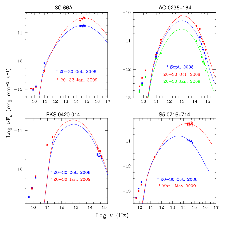
Figure 1: The modelled SED curves of the blazars 3C 66A, AO 0235$+$164, PKS 0420$-$014 and S5 0716$+$716. The points represent the observed data while the best fitted model is shown by line. Since the low frequency part ($\leq 10^{11}$ Hz) of blazars SEDs is governed by synchrotron-self absorption mechanism, so the modelled SED is steeper below a frequency of 10¹¹ Hz (see text for details).

S5 0716$+$714
S5 0716+714 was identified as an ISP (Giommi et al., 1999), at z = 0.31 $\pm$ 0.08 (Nilsson et al., 2008). However, Nieppola et al. (2006) studied the SED distribution of a large sample of BL Lac objects and categorized 0716$+$714 as a LSP. Two strong $\gamma$-ray flares on September and October 2007 from the source have been detected by AGILE (Giommi et al., 2008; Chen et al., 2008). They have also carried out the SED modelling of source with two synchrotron self-Compton (SSC) emission models, representative of a slowly and a rapidly variable component, respectively. Villata et al. (2008) reported optical-IR SED study of the source during the GASP-WEBT-AGILE campaign in 2007. Gupta et al. (2009) found high probabilities of quasi-periodic components of $\sim$25$-$73 minutes in the optical light curves observed by Montagni et al. (2006). Recently, nearly periodic oscillations of $\sim$15 minutes have been reported in the optical light curve of the source by Rani et al. (2010a).

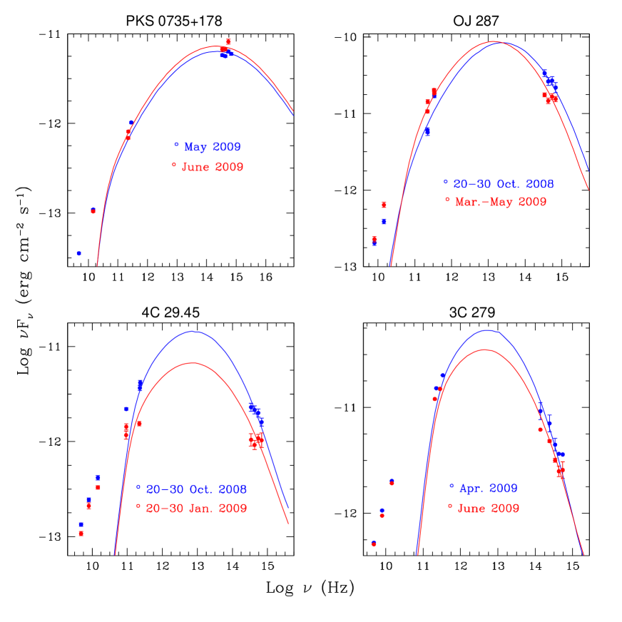
Figure 2: The modelled SED curves of the blazars PKS 0735$+$178, OJ 287, 4C 29.45 and 3C 279.

PKS 0735$+$178
PKS 0735$+$718 is a highly variable quasar and belongs to the category of BL Lac objects (Carswell et al., 1974). There have been several papers concerning its redshift determination (e.g. Carswell et al., 1974; Falomo & Ulrich, 2000, and the references therein) with the most recent result of $z=0.424$ for PKS 0735$+$718 found using a Hubble Space Telescope (HST) snapshot image (Sbarufatti et al., 2005); using that redshift, we classify this source as an ISP. The synchrotron part of SED of the source peaks at IR-UV, while the low X-ray variability with respect to the high optical-IR variations, supports the idea that X-rays are produced by an inverse Compton mechanism (Bregman et al., 1984; Madejski & Schwartz, 1988). Using ten year long multiband optical data of this source Ciprini et al. (2007) studied the multicolour behaviour, spectral index variations and their correlations with brightness.

OJ 287
OJ 287 (0851$+$202) (z = 0.306) is among the most extensively observed and best studied BL Lac objects with respect to variability. As it is very bright, it is among the very few AGN’s whose optical observations are available for more than a century (Sillanpaa et al., 1996; Gupta et al., 2008). A binary black hole model has been proposed to explain the $\sim$12 years optical periodicity (Sillanpaa et al., 1996; Valtonen et al., 2008). An intense optical, infrared, and radio variability study of the source for a time period between 1993 to 1998 was been reported in Pursimo et al. (2000). They detected two major optical outbursts in November 1994 and December 1995 even though the radio flux was very low during the period of outbursts. Using the multi-waveband flux and linear polarization observations and combining with sub-mm polarimetric images, Agudo et al. (2011) argued that the location of the $\gamma$-ray emission in prominent flares is $>$ 14 pc from the central black hole.

4C 29.45
4C 29.45 (z = 0.729; Wills et al., 1983), belongs to the category of FSRQs. Short and long term variability at both IR and optical bands has been observed in this source (Noble & Miller, 1996; Ghosh et al., 2000). Its optical flux and multi-colour variations were studied by Fan et al. (2006). They reported amplitude variations of $\sim$4.5$-$6 mag in all passbands (U, B, V, R, I) and also suggested that there were possible periods of 3.55 and 1.58 yr in the long-term optical LC of the source. The short term multi-band optical colour-brightness studies showed that the source tend to be redder with increase in its brightness (Rani et al., 2010b). Very recently, a GeV flare has been detected in this blazar (Ciprini, 2010).

3C 279
3C 279 is both one of the most extensively observed and most violent variable FSRQs across the whole electromagnetic spectrum; it is at a redshift of $z=0.536$. A comparison of radio to Gamma-ray SEDs of the source during low and high states of activity in the WEBT campaign of 2006 is presented in Böttcher et al. (2007). Collmar et al. (2010) carried out multifrequency variability study of source during January 2006. A complete compilation of all simultaneous SEDs of 3C 279 collected during the lifetime of CGRO, including modelling of those SEDs with a leptonic jet model, is presented in Hartman et al. (2001). Recently, Abdo et al. (2010a) report the coincidence of a $\gamma$-ray flare with a dramatic change of optical polarization angle. This provides evidence for co-spatial of optical and $\gamma$-ray emission regions and indicates a highly ordered jet magnetic field.

PKS 1510$-$089
PKS 1510$-$089 is classified as a FSRQ at a redshift of z = 0.361 (Thompson et al., 1990). It also belongs to the category of highly polarized quasars and already detected in the MeV–GeV energy band by the EGRET instrument on board the Compton Gamma-Ray Observatory (Hartman et al., 1992). The inverse Compton component dominated by the $\gamma$-ray emission, and the synchrotron emission peaked around IR frequencies, even if there is clearly visible in this source a pronounced UV bump, possibly caused by the thermal emission from the accretion disk (Malkan & Moore, 1986; Pian & Treves, 1993). The multi-wavelength flux and SED variability study of the source during its high $\gamma$-ray activity period between 2008 September and 2009 June has been reported by Abdo et al. (2010a). Recently, D’Ammando et al. (2011) reported the detailed analysis of multi-frequency coverage of extreme gamma-ray activity from the source observed by AGILE in March 2009. They have also carried out broad band SED study of the source and found thermal features in the optical/UV spectrum of the source during high $\gamma$-ray state.

3C 454.3
3C 454.3 is a FSRQ at a redshift of $z=0.859$, and is one of the most intense and variable of these sources (Pian et al., 2006; Villata et al., 2007; Gupta et al., 2008, and references therein). It is the brightest and most variable blazar at GeV energies (e.g. Vercellone et al., 2008; Raiteri et al., 2008; Vercellone et al., 2010). The multi-flare variability and SED study of the source in December 2007 and December 2009 is reported by Donnarumma et al. (2009) and Pacciani et al. (2010), respectively. The flaring behaviour of the source across the whole electromagnetic spectrum is studied by Jorstad et al. (2010). They conclude that the emergence of a superluminal knot from the core yields a series of optical and high-energy outbursts, and that the millimetre-wave core lies at the end of the jet’s acceleration and collimation zone.

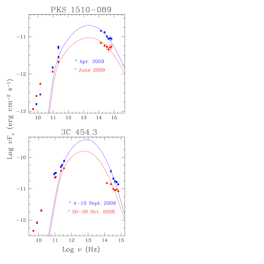
Figure 3: Modelled SED curves of the blazars PKS 1510$-$089 and 3C 454.3. The last three points in all of these SEDs are almost certainly dominated by contribution from the disk emission, so we exclude these points while modelling the SEDs of these two FSRQs.

5 Discussion

5.1 Statistical particle acceleration and log-parabolic spectra

Massaro et al. (2004) showed that when the acceleration efficiency is inversely proportional to the accelerating particle’s energy itself, then the energy distribution function, i.e., spectrum, approaches a log-parabolic shape. So, the log-parabolic spectra are naturally produced when the probability of statistical acceleration is energy dependent. According to this model, the curvature of emitting electron population ($r$) is related to fractional acceleration gain ($\epsilon$) as r $\propto$ 1/$\epsilon$. Also, E_P $\propto$ $\epsilon$ follows a negative trend between E_P and $b$ (see Tramacere et al., 2009), where E_P is the peak energy of observed SEDs.

So, if the above analysis is correct, then one should expect a negative trend between E_P or $\nu_{P}$ and $b$, where $\nu_{P}$ is the peak frequency of observed SEDs. We analysed the correlation between the two quantities using our data and found a significant negative correlation between $\nu_{P}$ and $b$ with $r_{P}=-0.74$ and $p$-value = 0.00014, where $r_{P}$ is the linear Pearson correlation coefficient and the $p$-value for the null hypothesis of no correlation corresponds to a significance level $>$ 99.98$\%$ (Fig. 4). So our result confirms that the spectral curvature parameter decreases as E_P moves towards higher energies and means that the blazars’ spectra in our cases are fit well by the log-parabolic model.

On the other hand, such a connection of log-parabolic spectra with acceleration may be also understood in the framework provided by the Fokker-Planck equation with momentum diffusion term (Kardashev et al., 1962; Massaro et al., 2006; Tramacere et al., 2009). They showed that the log-parabolic spectrum results from a Fokker-Planck equation with a momentum diffusion term and a mono-energetic or quasi-monoenergetic injection where the diffusion term acts to broaden the shape of the peak of the distribution. Kardashev et al. (1962) showed that the curvature term, $r\propto 1/(Dt)$ where $D$ is the Diffusion term. This relation leads to the following trend (Tramacere et al., 2009) :

$$ln(E_{P})=2~{}ln(\gamma_{P})+\frac{3}{5b}$$ (5)

So the both the momentum-diffusion term, $D$, and the fractional acceleration gain term, $\epsilon$, can explain the anti-correlation between $E_{P}$ and $b$.

An interesting check if the log-parabolic curve is actually related to the statistical acceleration is the existence of a linear relation between the two spectral parameters $a$ and $b$ (Massaro et al., 2004). So we checked the correlation among these two quantities and found that they are significantly correlated, with $r_{P}=0.61$ and $p$-value = 0.003 (see Fig. 5). So, we consider that in our case the log-parabola type spectra are very likely to be characterized by a full statistical acceleration mechanism working on the emitting electrons.

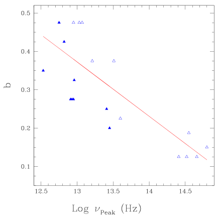
Figure 4: Curvature ($b$) vs peak frequency ($\nu_{P}$). A clear relation can be seen between the two quantities which is confirmed by a correlation analysis. The open symbols in this and subsequent figures represent BL Lacs while the filled symbols stand for FSRQs. The straight line is the best linear fit with a slope, $m=-0.14$ and constant, $c=2.22$ ($y=mx+c$).

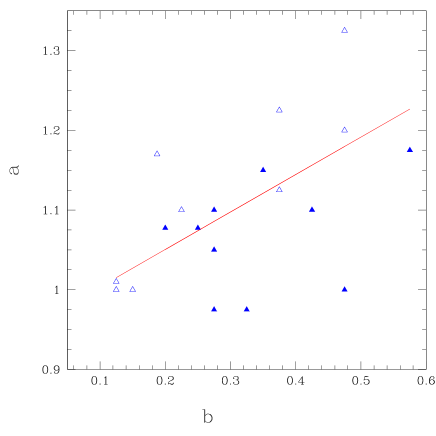
Figure 5: The spectral parameters, $a$ and $b$. A clear relation can be seen between the two quantities which is confirmed by a correlation analysis. The straight line is the best linear fit with $m=0.47$ and $c=0.96$.

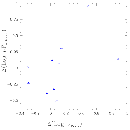
Figure 6: Changes in the peak intensity vs. change in peak frequency for all blazars (both BL Lacs and FSRQs together). There is no significant correlation found between the two quantities.

5.2 The cause of blazar SED changes

There are several possibilities that could be invoked to explain the changes in the synchrotron spectra. In the following sub-sections, we will discuss some of them in detail.

5.2.1 Evolution of the particle energy density distribution

The energy loss of the emitting particles is known to follow $\frac{d\gamma}{dt}$ $\cong$ $-$C$\gamma^{2}$ where $\gamma$ is the Lorentz factor and $C$ is a constant for both the synchrotron and IC emission (Rybicki & Lightman, 1979). The evolution of the relativistic particles can be described by energy-dependent Fokker-Planck equation (see for instance Kembhavi & Narlikar, 1999, p.52) :

$$\frac{\partial(\gamma,t)}{\partial t}=-\frac{\partial}{\partial\gamma}\Bigg{(}\frac{d\gamma}{dt}n(\gamma,t)\Bigg{)}+Q(\gamma,t)$$ (6)

where n($\gamma$,t) is the electron density distribution (a function of energy and time) and Q($\gamma$,t) is the time-dependent injection rate. The solutions to the equation above are typically rather complex and can be obtained in terms of Green’s functions for the general case.

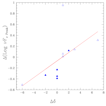
Figure 7: Changes in the peak intensity vs. change in Doppler factor for all blazars that have multiple SEDs in our sample. There is a clear relation seen between the two quantities.The straight line is the best linear fit with $m=0.07$ and $c=-0.07$.

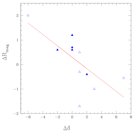
Figure 8: Changes in the R band magnitude vs. change in Doppler factor for all blazars that have multiple SEDs in our sample. There is a significant correlation between the two quantities, with $r_{P}=-0.70$ and $p$-value = 0.01. The straight line is the best linear fit with $m=-0.23$ and $c=0.29$.

If the changes in the blazar SEDs are due to a gradual change of the electron energy density distribution due to the synchrotron and IC losses, with no other injections meanwhile, then one should see both a total synchrotron energy decrease and mostly a decrease in $\gamma_{b}$ of the electron energy distribution (and respectively $-$ the frequency of the synchrotron peak emission). On the other hand, freshly injected electrons between the observational epochs (their energy should be higher than the average as it is expected to decrease in time) should reflect in the opposite behaviour (higher synchrotron emission and a peak blue-shift). So, in general one should expect to see a relation between the peak intensity and the peak frequency changes. To search for such a relation we used correlation analysis statistics (see Fig. 6). The correlation statistics revealed that there is no significant correlation between the two quantities as $r_{P}=0.54$ corresponding to a $p$-value = 0.084, where $r_{P}$ is the linear Pearson correlation coefficient and $p$ is a null hypothesis probability value. As there is no significant relation found between the two quantities, perhaps electron energy density evolution/electron injection is not the primary driver of the SED changes.

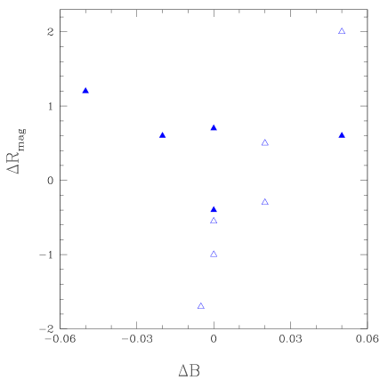
Figure 9: Changes in the R band magnitude vs. change in magnetic field for all blazars that have multiple SED’s in our sample. There is no significant correlation between the two quantities with $r_{P}=0.11$ and $p$-value = 0.75.

5.2.2 Change of the Doppler boosting factor

Another effect that can modify the blazar synchrotron emission is the change of the Doppler boosting factor, presumably due to a change either the bulk velocity or the viewing angle. Raiteri et al. (2010) also found that only geometrical (Doppler factor) changes are capable of explaining SED variations between two epochs for BL Lac. The changes of the synchrotron peak intensity vs. Doppler factor variations for our sample of blazars are shown in Fig. 7. We can see a clear relation among the two quantities and it is confirmed by values of $r_{P}=0.51$ and $p$-value = 0.05. We also searched for a correlation between change in R band magnitude vs. change in respective Doppler factor values. This would be relevant if $<$R$>$ is a somewhat more representative quantity for the synchrotron emission rather than peak intensity. Again, we found significant correlation among $\Delta$$R_{mag}$ and $\Delta$$\delta$ (see Fig. 8). So we consider that Doppler factor changes are a strong driver that can be responsible for the SED changes.

5.2.3 Change of the Magnetic Field

Since the value of the magnetic field, $B$ is related to the location of the dissipation region, if the two SEDs arise from periods of different activity it is quite possible that the emission was produced by blob that dissipates at different location in the jet. In that case we expect to find different $B$ values for the different SEDs of our sources. The change in $B$ values can also lead to variations in the flux of these sources which will be reflected in the two different SEDs of the sources. So we search for a correlation between the change in $<$R$>$ and that in $B$ (Fig. 9) but we do not find any significant correlation among them for all of out blazars. However, we notice an apparent significant correlation among these two parameters for the BL Lacs alone, which is confirmed by correlation analysis ($r_{P}=0.96$, $p=0.002$ for BL Lacs). So we conclude that changes in magnetic field strength may be responsible for the SED changes in the case of BL Lacs.

6 Conclusions

We have carried out the radio to optical through mm, sub-mm and IR SED studies of a sample of ten blazars including five BL Lacs and five FSRQs, eight of which are LSPs and the other two ISPs. We modelled the SEDs of blazars using synchrotron spectra with log-parabolic distributions. We found a significant negative correlation among $\nu_{Peak}$ and the curvature term $r$, which implies that the acceleration efficiency of emitting electrons is inversely proportional to energy itself; however this correlation can also be explained by the momentum diffusion term in the solution of Fokker-Planck equation. Also, a significant correlation between the two spectral parameters $a$ and $b$, implies that the log-parabolic curve is likely to be related to the statistical acceleration of emitting electrons.

Of course our modelling has significant limitations. We are assuming that only one-zone dominates the emission at any given time, and this is unlikely to be an excellent approximation. Although we strived for data obtained simultaneously, this was often impossible to obtain; therefore any variations within the “high” and “low” states have been averaged over time bins ranging from days to two months. This lack of simultaneity could have vitiated our results but only appears to have added scatter to all of the Figures 4–9.

We considered each likely factor that could be responsible for the changes in observed SEDs of blazars. If the electron energy density evolution governs the SED changes then one should expect a correlation between change in peak intensity vs change in peak frequency. Since we do not observe any such correlation we consider that probably the evolution of electron energy density cannot be responsible for the observed SED changes. Also for our entire sample of blazars, changes in $<$R_mag$>$ are not correlated with the respective changes in $B$, so the change in magnetic field strength is probably not responsible for the SED changes we saw. However, for the BL Lacs alone the SED changes may be driven by changes in $B$. We find that the change in Doppler factor is significantly correlated with the change in peak intensity as well as with $<$R_mag$>$. So it is reasonable to suggest that the change in Doppler factor (either bulk velocity or viewing angle) is the primary driver that governs the SED changes in short term variability (STV) in blazars.

References

- Abdo et al. (2010a) Abdo, A. A., et al. 2010a, \apj, 721, 1425
- Abdo et al. (2010b) Abdo, A. A., et al. 2010b, \apj, 716, 30
- Abdo et al. (2010c) Abdo, A. A., et al. 2010c, \apjs, 188, 405
- Agudo et al. (2011) Agudo, I., et al. 2011, \apjl, 726, L13
- Bach et al. (2010) Bach, U., Fuhrmann, L., Konstantinova, T., Larionov, V. M., Raiteri, C. M., Villata, M., & Leto, P. 2010, The Astronomer’s Telegram, 2395, 1
- Błażejowski et al. (2000) Błażejowski, M., Sikora, M., Moderski, R., & Madejski, G. M. 2000, \apj, 545, 107
- Böttcher et al. (2007) Böttcher, M., et al. 2007, \apj, 670, 968
- Böttcher et al. (2009) Böttcher, M., et al. 2009, \apj, 694, 174
- Böttcher et al. (2005) Böttcher, M., et al. 2005, \apj, 631, 169
- Bramel et al. (2005) Bramel, D. A., et al. 2005, \apj, 629, 108
- Bregman et al. (1984) Bregman, J. N., et al. 1984, \apj, 276, 454
- Carswell et al. (1974) Carswell, R. F., Strittmatter, P. A., Williams, R. E., Kinman, T. D., & Serkowski, K. 1974, \apjl, 190, L101
- Chen et al. (2008) Chen, A. W., et al. 2008, \aap, 489, L37
- Ciprini (2010) Ciprini, S. 2010, The Astronomer’s Telegram, 2795, 1
- Ciprini et al. (2007) Ciprini, S., et al. 2007, \aap, 467, 465
- Collmar et al. (2010) Collmar, W., et al. 2010, \aap, 522, A66
- D’Ammando et al. (2011) D’Ammando F., et al., 2011, A&A, 529, A145
- Dermer & Schlickeiser (1993) Dermer, C. D., & Schlickeiser, R. 1993, \apj, 416, 458
- Donnarumma et al. (2009) Donnarumma, I., et al. 2009, \apj, 707, 1115
- Falomo & Ulrich (2000) Falomo, R., & Ulrich, M. 2000, \aap, 357, 91
- Fan et al. (2006) Fan, J., et al. 2006, \pasj, 58, 945
- Ghisellini et al. (1999) Ghisellini, G., et al. 1999, \aap, 348, 63
- Ghisellini et al. (1996) Ghisellini, G., Maraschi, L., & Dondi, L. 1996, \aaps, 120, C503
- Ghisellini et al. (1993) Ghisellini, G., Padovani, P., Celotti, A., & Maraschi, L. 1993, \apj, 407, 65
- Ghisellini et al. (1997) Ghisellini, G., et al. 1997, \aap, 327, 61
- Ghosh et al. (2000) Ghosh, K. K., Ramsey, B. D., Sadun, A. C., & Soundararajaperumal, S. 2000, \apjs, 127, 11
- Giommi et al. (1999) Giommi, P., et al. 1999, \aap, 351, 59
- Giommi et al. (2008) Giommi P., et al., 2008, A&A, 487, L49
- Gupta et al. (2008) Gupta, A. C., Fan, J. H., Bai, J. M., & Wagner, S. J. 2008, \aj, 135, 1384
- Gupta et al. (2009) Gupta, A. C., Srivastava, A. K., & Wiita, P. J. 2009, \apj, 690, 216
- Hagen-Thorn et al. (2008) Hagen-Thorn, V. A., Larionov, V. M., Jorstad, S. G., Arkharov, A. A., Hagen-Thorn, E. I., Efimova, N. V., Larionova, L. V., & Marscher, A. P. 2008, \apj, 672, 40
- Hartman et al. (1992) Hartman, R. C., et al. 1992, \apjl, 385, L1
- Hartman et al. (2001) Hartman, R. C., et al. 2001, \apj, 553, 683
- Hovatta et al. (2009) Hovatta, T., Valtaoja, E., Tornikoski, M., & Lähteenmäki, A. 2009, \aap, 494, 527
- Jorstad et al. (2010) Jorstad, S. G., et al. 2010, \apj, 715, 362
- Joshi & Böttcher (2007) Joshi, M., & Böttcher, M. 2007, \apj, 662, 884
- Kardashev et al. (1962) Kardashev, N. S., Kuz’min, A. D., & Syrovatskii, S. I. 1962, \sovast, 6, 167
- Kembhavi & Narlikar (1999) Kembhavi A. K., Narlikar J. V., 1999, Quasars and active galactic nuclei., ed. Kembhavi, A. K. & Narlikar, J. V. Cambridge Univ. Press, Cambridge
- Kuehr et al. (1981) Kuehr, H., Witzel, A., Pauliny-Toth, I. I. K., & Nauber, U. 1981, \aaps, 45, 367
- Madejski & Schwartz (1988) Madejski, G. M., & Schwartz, D. A. 1988, \apj, 330, 776
- Malkan & Moore (1986) Malkan, M. A., & Moore, R. L. 1986, \apj, 300, 216
- Malkan & Sargent (1982) Malkan, M. A., & Sargent, W. L. W. 1982, \apj, 254, 22
- Maraschi et al. (1992) Maraschi, L., Ghisellini, G., & Celotti, A. 1992, \apjl, 397, L5
- Marscher & Gear (1985) Marscher, A. P., & Gear, W. K. 1985, \apj, 298, 114
- Massaro et al. (2004) Massaro, E., Perri, M., Giommi, P., & Nesci, R. 2004, \aap, 413, 489
- Massaro et al. (2006) Massaro, E., Tramacere, A., Perri, M., Giommi, P., & Tosti, G. 2006, \aap, 448, 861
- Miller et al. (1978) Miller, J. S., French, H. B., & Hawley, S. A. 1978, \apjl, 219, L85
- Montagni et al. (2006) Montagni, F., Maselli, A., Massaro, E., Nesci, R., Sclavi, S., & Maesano, M. 2006, \aap, 451, 435
- Mukherjee et al. (1999) Mukherjee, R., et al. 1999, \apj, 527, 132
- Nilsson et al. (1996) Nilsson, K., Charles, P. A., Pursimo, T., Takalo, L. O., Sillanpaeae, A., & Teerikorpi, P. 1996, \aap, 314, 754
- Nilsson et al. (2008) Nilsson, K., Pursimo, T., Sillanpää, A., Takalo, L. O., & Lindfors, E. 2008, \aap, 487, L29
- Noble & Miller (1996) Noble, J. C., & Miller, H. R. 1996, in Astronomical Society of the Pacific Conference Series, Vol. 110, Blazar Continuum Variability, ed. H. R. Miller, J. R. Webb, & J. C. Noble, 30
- Pacciani et al. (2010) Pacciani, L., et al. 2010, \apjl, 716, L170
- Padovani & Giommi (1995) Padovani, P., & Giommi, P. 1995, \mnras, 277, 1477
- Petry et al. (2000) Petry, D., et al. 2000, \apj, 536, 742
- Pian et al. (2006) Pian, E., et al. 2006, \aap, 449, L21
- Pian & Treves (1993) Pian, E., & Treves, A. 1993, \apj, 416, 130
- Pilbratt et al. (2010) Pilbratt, G. L., et al. 2010, \aap, 518, L1
- Pursimo et al. (2000) Pursimo, T., et al. 2000, \aaps, 146, 141
- Raiteri et al. (1998) Raiteri, C. M., Ghisellini, G., Villata, M., de Francesco, G., Lanteri, L., Chiaberge, M., Peila, A., & Antico, G. 1998, \aaps, 127, 445
- Raiteri et al. (2010) Raiteri, C. M., et al. 2010, \aap, 524, A43
- Raiteri et al. (2006) Raiteri, C. M., et al. 2006, \aap, 459, 731
- Raiteri et al. (2008) Raiteri, C. M., et al. 2008, \aap, 480, 339
- Rani et al. (2010a) Rani, B., Gupta, A. C., Joshi, U. C., Ganesh, S., & Wiita, P. J. 2010a, \apjl, 719, L153
- Rani et al. (2011) Rani B., Gupta A. C., Joshi U. C., Ganesh S., Wiita P. J., 2011, MNRAS, 413, 2157
- Rani et al. (2010b) Rani, B., et al. 2010b, \mnras, 404, 1992
- Rani et al. (2009) Rani, B., Wiita, P. J., & Gupta, A. C. 2009, \apj, 696, 2170
- Rybicki & Lightman (1979) Rybicki G. B., Lightman A. P., 1979, Radiative processes in astrophysics, ed. Rybicki, G. B. & Lightman, A. P.
- Sbarufatti et al. (2005) Sbarufatti, B., Treves, A., & Falomo, R. 2005, \apj, 635, 173
- Sikora (1994) Sikora, M. 1994, \apjs, 90, 923
- Sillanpaa et al. (1996) Sillanpaa, A., et al. 1996, \aap, 305, L17
- Sohn et al. (2003) Sohn, B. W., Klein, U., & Mack, K. 2003, \aap, 404, 133
- Tavecchio et al. (2002) Tavecchio, F., et al. 2002, \apj, 575, 137
- Teräsranta et al. (2004) Teräsranta, H., et al. 2004, \aap, 427, 769
- Thompson et al. (1990) Thompson, D. J., Djorgovski, S., & de Carvalho, R. 1990, \pasp, 102, 1235
- Tramacere et al. (2007) Tramacere, A., et al. 2007, \aap, 467, 501
- Tramacere et al. (2009) Tramacere, A., Giommi, P., Perri, M., Verrecchia, F., & Tosti, G. 2009, \aap, 501, 879
- Valtonen et al. (2008) Valtonen, M. J., et al. 2008, \nat, 452, 851
- Vercellone et al. (2008) Vercellone, S., et al. 2008, \apjl, 676, L13
- Vercellone et al. (2010) Vercellone, S., et al. 2010, \apj, 712, 405
- Villata et al. (2007) Villata, M., et al. 2007, \aap, 464, L5
- Villata et al. (1997) Villata, M., et al. 1997, \aaps, 121, 119
- Villata et al. (2008) Villata, M., et al. 2008, \aap, 481, L79
- Webb et al. (1988) Webb, J. R., Smith, A. G., Leacock, R. J., Fitzgibbons, G. L., Gombola, P. P., & Shepherd, D. W. 1988, \aj, 95, 374
- Wills et al. (1983) Wills, B. J., et al. 1983, \apj, 274, 62
- Yan et al. (2010) Yan, D., Fan, Z., & Dai, B. 2010, arXiv, arXiv:1011.1537