Turbulent transition in a truncated 1D model for shear flow

Abstract

fluid flow; turbulence; dynamical systems We present a reduced model for the transition to turbulence in shear flow that is simple enough to admit a thorough numerical investigation while allowing spatio-temporal dynamics that are substantially more complex than those allowed in previous modal truncations.

Our model allows a comparison of the dynamics resulting from initial perturbations that are localised in the spanwise direction with those resulting from sinusoidal perturbations. For spanwise-localised initial conditions the subcritical transition to a ‘turbulent’ state (i) takes place more abruptly, with a boundary between laminar and ‘turbulent’ flow that is appears to be much less ‘structured’ and (ii) results in a spatiotemporally chaotic regime within which the lifetimes of spatiotemporally complicated transients are longer, and are even more sensitive to initial conditions.

The minimum initial energy $E_{0}$ required for a spanwise-localised initial perturbation to excite a chaotic transient has a power-law scaling with Reynolds number $E_{0}\sim Re^{p}$ with $p\approx-4.3$. The exponent $p$ depends only weakly on the width of the localised perturbation and is lower than that commonly observed in previous low-dimensional models where typically $p\approx-2$.

The distributions of lifetimes of chaotic transients at fixed Reynolds number are found to be consistent with exponential distributions.

1 Introduction

The transition from laminar to turbulent states has been a central problem in fluid mechanics for many decades. Since the 1960s, promising lines of attack have been opened up through the use of ideas from dynamical systems theory coupled to the thorough investigation of reduced versions of the Navier–Stokes equations. Perhaps the best-known example of such a reduction is the derivation of the Lorenz equations as a model of the onset of thermal convection in a layer of fluid heated from below (Lorenz 1963). Although the set of three nonlinear ODEs that comprise the Lorenz 1963 model displays a wealth of interesting dynamical behaviour, little of this is relevant to the original fluid-mechanical problem. However, similar approaches yield convincing agreement over wide ranges of parameter values in other fluid-mechanical situations, for example thermal convection in the presence of a magnetic field, and the onset of Taylor vortices in the flow between rotating coaxial concentric cylinders. In situations such as these the flow undergoes a series of bifurcations before becoming chaotic, in a sense that can be given a clear meaning in terms of the behaviour of the reduced model comprising nonlinear ODEs.

In contrast, the transition to turbulence in shear flows appears not to proceed through a sequence of bifurcations, but to be linked to the appearance, at a critical Reynolds number $Re_{c}$, of a chaotic saddle in phase space: a complicated collection of unstable equilibria and time-periodic orbits which results in ever longer transients before the flow relaxes to a purely laminar state. For a review, and substantial numbers of references to the literature (although with an emphasis on pipe flow), see Kerswell (2005). The significance of $Re_{c}$ is that for $Re<Re_{c}$ the laminar state is a global attractor and trajectories appear to evolve rapidly towards it, while for $Re>Re_{c}$ other (usually unstable) invariant sets exist in phase space. These new invariant sets cause increasingly long transient excursions to take place before relaminarisation occurs, for initial conditions that are sufficiently far from the laminar profile. Small perturbations to the laminar state still decay rapidly towards it, and there appears to be a distinct boundary separating the behaviour of trajectories into those that relax rapidly and those which undergo long transient excursions. This laminar-turbulent boundary is sometimes referred to as the ‘edge of chaos’. Despite these differences in phenomenology and dynamics, reduced models constructed along the same lines as the Lorenz model have provided substantial insight into both the physical origin of this transition to self-sustaining complicated motion, and the mathematical organisation of equilibria and periodic orbits inside the chaotic saddle.

The study by Waleffe (1997) provides the direct inspiration for the present work. Waleffe showed that a low-order reduced model could be constructed that elucidated the different elements of a self-sustaining process (SSP) that allowed sufficiently large deviations from the laminar flow profile to persist indefinitely. The SSP can be briefly described as follows. Weak streamwise vortices (i.e. vortical rolls whose axes are aligned with the primary flow direction) distort the streamwise velocity profile by moving high and low-speed fluid around. This distortion generates streamwise streaks of fluid that are moving faster and slower than the fluid around them. The streaks are unstable to modes which create vortical eddies oriented in the wall-normal direction, orthogonal to the streamwise vortices, and the resulting three-dimensional re-organisation of the flow reinforces the streamwise vortices.

Waleffe’s model simplified the Navier–Stokes equations first by considering, not plane Couette flow between rigid boundaries, but a modified problem in which the boundaries are stress-free and the laminar profile is sinusoidal, sustained by an artificially-applied pressure term. It appears that the physics of the SSP is rather insensitive to these modifications. The second set of simplifications concern the Galerkin expansion of the velocity field in all three directions: streamwise ($x$), wall normal ($y$) and spanwise ($z$). Thus Waleffe considered a model comprising 8 of the lowest-wavenumber Fourier modes in this Galerkin expansion. These 8 modes were chosen in order to capture the central elements of the SSP, and to be self-consistent in the sense that the nonlinear (quadratic) interactions between these 8 modes preserve energy just as the full advective nonlinearity in the Navier–Stokes equations does. Having projected out the spatial dependence of the dynamics onto these modes, the problem reduces to a far simpler set of ordinary differential equations (ODEs) for the time-dependent mode amplitudes. Subsequent work, in particular by Eckhardt & Mersmann (1999) and Moehlis, Faisst and Eckhardt (2004, 2005) extended Waleffe’s model to include an additional physical insight: that the basic laminar profile of the shear flow will itself be modified by the nonlinear interactions with streamwise vortices and streaks. Moehlis et al developed a 9-mode ODE model that was amenable to investigation in substantial detail. In particular they discussed the lifetimes of perturbations as the Reynolds number increased, locating the onset of complicated dynamics, and they also discussed the probabilistic distribution of lifetimes at fixed Reynolds number from randomised initial conditions of equal energy.

It is clear that the assumptions made by these authors concerning spatial periodicity seems much easier to argue for in the streamwise and wall-normal directions than in the spanwise direction; indeed recent work by Schneider and co-workers (Schneider et al 2009; 2010a; 2010b) (see also Duguet, Schlatter and Henningson, 2009) has concentrated on understanding the formation of structures which are spatially localized in $z$: very far from periodic in this direction.

With this in mind we propose in this paper an extension of Waleffe’s model which is a reduction of the Navier–Stokes equations to a collection of PDEs in $z$ and $t$: we adopt the Fourier mode truncations that Waleffe used in order to remove the dependence on the streamwise $x$ and wall-normal $y$ coordinates since numerical work shows that, at least for some of these equilibrium and periodic orbit states, the flow structure in these coordinates can be well-approximated by a small number of Fourier modes.

By retaining full dependence on the spanwise coordinate $z$ we admit both the spatially-periodic solutions of Waleffe and the formation of localized states. In addition, a wealth of spatio-temporal complexity is allowed. Our study is very similar in spirit to work by Manneville and co-authors (Manneville & Locher 2000; Manneville 2004; Lagha & Manneville 2007) who preserve full resolution in two directions (streamwise and spanwise) and use Galerkin truncation only in the third (‘wall-normal’) direction. This enables these authors to consider the dynamics around turbulent spots that are localised in both the streamwise and spanwise directions, at the cost of more intensive numerical computations. Their work is therefore complementary to that presented here. We remark also that reduced models, of different kinds, have been used both in pipe flow (Willis & Kerswell 2009) and in understanding the formation of turbulent-laminar bands in plane Couette flow (Barkley & Tuckerman 2007).

The structure of the paper is as follows. In section 2 we discuss the derivation of our PDE extension of Waleffe’s ODE model. In section 3 we present the results of our numerical investigations into the transition to turbulence described by the model. We conclude in section 4.

2 Derivation of the PDE model

In this section we define sinusoidal shear flow and summarise the Galerkin truncation that we use to derive our simplified model for turbulent transition.

Following Waleffe (1997) and Moehlis et al (2004), we use the usual Cartesian coordinate conventions that $x$ is the downstream direction (‘streamwise’), $y$ is the direction of the shear gradient, i.e. normal to the sidewalls and $z$ is the spanwise direction. We write the Navier–Stokes equations for incompressible flow in the nondimensionalised form

$$\frac{\partial\mathbf{u}}{\partial t}+\mathbf{u}\cdot\nabla\mathbf{u}=-\nabla p+\mathbf{F}(y)+\frac{1}{Re}\nabla^{2}\mathbf{u},$$ (1)

where we have scaled lengths by $h/2$ where $h$ is the width of the channel, velocities by $U_{0}$ the velocity of the laminar profile at a distance $h/4$ from the upper boundary and pressure by $U_{0}^{2}\rho$ where $\rho$ is the density of the fluid. The Reynolds number $Re$ is therefore given by $Re=U_{0}h/(2\nu)$, $\nu$ being the kinematic viscosity. The evolution of (1) is subject to the usual incompressibility condition $\nabla\cdot\mathbf{u}=0$ and the conditions for impermeable and stress-free upper and lower boundaries

$$u_{y}=0,\qquad\mathrm{and}\qquad\frac{\partial u_{x}}{\partial y}=\frac{\partial u_{z}}{\partial y}=0\qquad\mathrm{at}\qquad y=\pm 1.$$ (2)

The flow is assumed to be periodic in the $x$ and $z$ directions, with periodicities $L_{x}$ and $L_{z}$ respectively. We take the body force term $\mathbf{F}(y)$ to be

$$\mathbf{F}(y) = \frac{\sqrt{2}\beta^{2}}{Re}\sin\beta y\,\mathbf{e}_{x},$$ (3)

where $\mathbf{e}_{x}$ is the unit vector in $x$ direction and it is convenient to define the constant $\beta=\pi/2$. The laminar profile is then the steady solution

$$\mathbf{u} = \sqrt{2}\sin\beta y\mathbf{e}_{x},$$ (4)

of (1) - (3), as shown in figure 1.

Figure 1: Geometry of the domain, illustrating the basic sinusoidal shear profile $\mathbf{u}=\sqrt{2}\sin\beta y\mathbf{e}_{x}$ which is sustained by the applied body force term.

We note that although the ‘sinusoidal shear flow’ profile (4) has an inflection point, the flow is linearly stable for all $Re$ (Drazin & Reid 1981).

We now turn to our solution ansatz. We write the velocity field in the form

$$\mathbf{u} = \mathbf{u}_{M}+\nabla\!\times\boldsymbol{\Phi}_{T}+\nabla\!\times\nabla\!\times\boldsymbol{\Phi}_{P},$$ (5)

where the subscripts denote mean, toroidal and poloidal components which are, respectively, expressed as sums of the first few Fourier modes in each case:

$$\mathbf{u}_{M} = \left(A_{1}\sin\beta y+A_{2}\right)\mathbf{e}_{x},$$

$$\boldsymbol{\Phi}_{T} = A_{3}\cos\beta y\,\mathbf{e}_{x}$$

$$+\left(A_{4}\sin\alpha x-A_{5}\cos\alpha x\sin\beta y-A_{6}\cos\alpha x+A_{7}\sin\alpha x\sin\beta y\right)\mathbf{e}_{y},$$

$$\boldsymbol{\Phi}_{P} = A_{8}\cos\alpha x\cos\beta y\,\mathbf{e}_{y}.$$

We define the streamwise and spanwise wavenumbers $\alpha=2\pi/L_{x}$ and $\gamma=2\pi/L_{z}$ for notational convenience. The amplitudes $A_{1},\ldots,A_{8}$ are functions of $z$ and $t$ whose evolution can be obtained by substituting (5) into (1). Note that the form of the ansatz implies that incompressibility and the boundary conditions (2) are automatically satisfied.

The amplitudes $A_{1},\ldots,A_{8}$ correspond exactly, in terms of their Fourier dependence in $x$ and $y$, to the modes selected by Waleffe (1997). For reference, table 1 summarises the correspondence.

Table 1: Comparison of notation.

This paper	$A_{1}$	$A_{2}$	$A_{3}$	$A_{4}$	$A_{5}$	$A_{6}$	$A_{7}$	$A_{8}$
Waleffe (1997)	$M$	$U$	$V$	$A$	$C$	$B$	$D$	$E$
	const	$\cos\gamma z$	$\sin\gamma z$	const	const	$\cos\gamma z$	$\cos\gamma z$	$\sin\gamma z$

We now briefly describe the role that each mode plays in the dynamics. $A_{1}$ is the amplitude of the sinusoidal shear profile; the laminar state corresponds to $A_{1}=\sqrt{2}$, $A_{2}=\cdots=A_{8}=0$. $A_{2}$ describes variations in $z$ of the streamwise velocity, i.e. the formation of streamwise streaks. $A_{3}$ describes the formation of $x$-independent streamwise vortices that redistribute the shear profile. Modes $A_{4},\ldots,A_{7}$ describe, as in Waleffe (1997) the development of $x$-dependent distortions of the streaks, and in particular the linear instability of the $x$-independent streaks described by $A_{2}$. These modes have no velocity component in the vertical (i.e. $y$) direction. $A_{8}$ describes ‘oblique rolls’ and, in contrast to modes $A_{4},\ldots,A_{7}$, has a non-zero vertical velocity component but no vertical vorticity component.

To derive evolution equations for the modes $A_{1},\ldots,A_{8}$ we use Fourier orthogonality in the $x$ and $y$ directions combined with projections onto individual components of either the velocity field $\mathbf{u}$, the vorticity field $\boldsymbol{\omega}=\nabla\!\times\mathbf{u}$ or (for $A_{8}$) the curl of the vorticity field. For later convenience we introduce the differential operators $\mathcal{D}_{\alpha}^{2}$, $\mathcal{D}_{\beta}^{2}$ and $\mathcal{D}_{\alpha\beta}^{2}$ which correspond to the action of $-\nabla^{2}$ on different Fourier modes:

$$\mathcal{D}_{\alpha}^{2}\equiv\alpha^{2}-\partial_{zz},\quad\mathcal{D}_{\beta}^{2}\equiv\beta^{2}-\partial_{zz},\quad\mathcal{D}_{\alpha\beta}^{2}\equiv\alpha^{2}+\beta^{2}-\partial_{zz}.$$

We denote $\partial A_{j}/\partial z$ by $A_{j}^{\prime}$ for $j=1,\ldots,8$. Considering first the $\mathbf{e}_{x}$ component of $\mathbf{u}$ in (1) we obtain the following PDEs in $z$ and $t$ for $A_{1}$ and $A_{2}$:

$$\left(\partial_{t}+\frac{1}{Re}\mathcal{D}_{\beta}^{2}\right)A_{1} = -\beta A_{2}^{\prime}A_{3}+\frac{\alpha}{2}(A_{4}^{\prime\prime}A_{5}-A_{4}A_{5}^{\prime\prime})+\frac{\alpha}{2}(A_{6}A_{7}^{\prime\prime}-A_{6}^{\prime\prime}A_{7})$$ (6)

$$+\frac{\beta}{2}(A_{6}^{\prime\prime}A_{8}^{\prime}-\alpha^{2}A_{6}A_{8}^{\prime})+\frac{\sqrt{2}\beta^{2}}{Re},$$

$$\left(\partial_{t}-\frac{1}{Re}\partial_{zz}\right)A_{2} = -\frac{\beta}{2}(A_{1}A_{3})^{\prime}+\frac{\alpha}{2}(A_{4}^{\prime\prime}A_{6}-A_{4}A_{6}^{\prime\prime})-\frac{\alpha}{4}(A_{5}^{\prime\prime}A_{7}-A_{5}A_{7}^{\prime\prime})$$ (7)

$$-\frac{\alpha^{2}\beta}{4}(A_{5}A_{8})^{\prime}+\frac{\beta}{4}(A_{5}^{\prime}A_{8}^{\prime})^{\prime},$$

Now we turn to the vorticity $\boldsymbol{\omega}$. For $A_{3}$, $A_{4}$ and $A_{6}$ we find that only one component of $\boldsymbol{\omega}$ contains a contribution from each of these; taking the curl of (5) the terms involving $A_{3}$, $A_{4}$ and $A_{6}$ are

$$\boldsymbol{\omega} = \mathcal{D}_{\beta}^{2}A_{3}\cos\beta y\,\mathbf{e}_{x}+\left(\mathcal{D}_{\alpha}^{2}A_{4}\sin\alpha x-\mathcal{D}_{\alpha}^{2}A_{6}\cos\alpha x\right)\mathbf{e}_{y}.$$

Therefore it is straightforward to consider the $x$ and $y$ components of the vorticity equation obtained by applying the operators $\mathbf{e}_{x}\cdot\nabla\!\times$ and $\mathbf{e}_{y}\cdot\nabla\!\times$ to (1) in order to obtain evolution equations for $A_{3}$, $A_{4}$ and $A_{6}$:

$$\left(\partial_{t}+\frac{1}{Re}\mathcal{D}_{\beta}^{2}\right)\mathcal{D}_{\beta}^{2}A_{3} = -\alpha^{2}\beta(A_{4}A_{7})^{\prime}-\alpha^{2}\beta(A_{5}A_{6})^{\prime}+\frac{\alpha^{3}}{2}(A_{4}A_{8})^{\prime\prime}$$ (8)

$$-\frac{\alpha}{2}(A_{4}A_{8}^{\prime\prime})^{\prime\prime}+\alpha\beta^{2}A_{4}^{\prime}A_{8}^{\prime}+\frac{\alpha^{3}\beta^{2}}{2}A_{4}A_{8}$$

$$+\frac{\alpha\beta^{2}}{2}A_{4}A_{8}^{\prime\prime},$$

$$\left(\partial_{t}+\frac{1}{Re}\mathcal{D}_{\alpha}^{2}\right)\mathcal{D}_{\alpha}^{2}A_{4} = \frac{\alpha}{2}(A_{1}A_{5}^{\prime\prime}-A_{1}^{\prime\prime}A_{5})-\frac{\alpha^{3}}{2}A_{1}A_{5}+\alpha(A_{2}A_{6}^{\prime\prime}-A_{2}^{\prime\prime}A_{6})$$ (9)

$$-\alpha^{3}A_{2}A_{6}+\frac{\beta}{2}(A_{3}A_{7}^{\prime})^{\prime\prime}-\frac{\alpha^{2}\beta}{2}A_{3}A_{7}^{\prime}-\alpha^{2}\beta A_{3}^{\prime}A_{7}$$

$$-\frac{\alpha^{3}\beta^{2}}{2}A_{3}A_{8}+\frac{\alpha\beta^{2}}{2}(A_{3}A_{8}^{\prime\prime}-A_{3}^{\prime\prime}A_{8}),$$

$$\left(\partial_{t}+\frac{1}{Re}\mathcal{D}_{\alpha}^{2}\right)\mathcal{D}_{\alpha}^{2}A_{6} = \frac{\alpha^{3}}{2}A_{1}A_{7}-\frac{\alpha}{2}(A_{1}A_{7}^{\prime\prime}-A_{1}^{\prime\prime}A_{7})+\alpha^{2}\beta A_{1}^{\prime}A_{8}$$ (10)

$$+\frac{\alpha^{2}\beta}{2}A_{1}A_{8}^{\prime}-\frac{\beta}{2}(A_{1}A_{8}^{\prime})^{\prime\prime}+\alpha^{3}A_{2}A_{4}$$

$$-\alpha(A_{2}A_{4}^{\prime\prime}-A_{2}^{\prime\prime}A_{4})+\frac{\beta}{2}(A_{3}A_{5}^{\prime})^{\prime\prime}-\alpha^{2}\beta A_{3}^{\prime}A_{5}$$

$$-\frac{\alpha^{2}\beta}{2}A_{3}A_{5}^{\prime},$$

Evolution equations for $A_{5}$, $A_{7}$ and $A_{8}$ are derived similarly, using (for $A_{5}$ and $A_{7}$) the projection operator $\mathbf{e}_{y}\cdot\nabla\!\times$ and (for $A_{8}$) the projection operator $\mathbf{e}_{y}\cdot\nabla\!\times\nabla\!\times$ applied to (1). The resulting evolution equations are

$$\left(\partial_{t}+\frac{1}{Re}\mathcal{D}_{\alpha\beta}^{2}\right)\mathcal{D}_{\alpha}^{2}A_{5} = \alpha^{3}A_{1}A_{4}-\alpha(A_{1}A_{4}^{\prime\prime}-A_{1}^{\prime\prime}A_{4})+\alpha^{3}A_{2}A_{7}$$ (11)

$$-\alpha(A_{2}A_{7}^{\prime\prime}-A_{2}^{\prime\prime}A_{7})-\beta(A_{2}^{\prime}A_{8}^{\prime})^{\prime}$$

$$+\alpha^{2}\beta A_{2}^{\prime}A_{8}-\alpha^{2}\beta(A_{3}A_{6})^{\prime}+\beta(A_{3}A_{6}^{\prime\prime})^{\prime},$$

$$\left(\partial_{t}+\frac{1}{Re}\mathcal{D}_{\alpha\beta}^{2}\right)\mathcal{D}_{\alpha}^{2}A_{7} = -\alpha^{3}A_{1}A_{6}+\alpha(A_{1}A_{6}^{\prime\prime}-A_{1}^{\prime\prime}A_{6})-\alpha^{3}A_{2}A_{5}$$ (12)

$$+\alpha(A_{2}A_{5}^{\prime\prime}-A_{2}^{\prime\prime}A_{5})+\beta(A_{3}A_{4}^{\prime\prime})^{\prime}$$

$$-\alpha^{2}\beta(A_{3}A_{4})^{\prime},$$

$$\left(\partial_{t}+\frac{1}{Re}\mathcal{D}_{\alpha\beta}^{2}\right)\mathcal{D}_{\alpha\beta}^{2}\mathcal{D}_{\alpha}^{2}A_{8} = -2\alpha^{2}\beta(A_{1}^{\prime}A_{6}+A_{2}^{\prime}A_{5})-2\alpha\beta^{2}A_{3}^{\prime}A_{4}^{\prime}$$ (13)

$$+\alpha(A_{3}^{\prime\prime}A_{4})^{\prime\prime}-\alpha(\alpha^{2}+\beta^{2})A_{3}^{\prime\prime}A_{4}.$$

Equations (6) - (13) are a closed set of nonlinear PDEs in $z$ and $t$ which form a truncated model of the dynamics of sinusoidal shear flow. Crucially these equations satisfy two consistency checks: the nonlinear terms in (6) - (13) conserve energy and so reflect the conservative nature of the full $\mathbf{u}\cdot\nabla\mathbf{u}$ nonlinearity in (1). Secondly this model reduces to the model of Waleffe (1997) in the special case in which the amplitudes $A_{1},\ldots,A_{8}$ are taken to be periodic in the $z$-direction, after applying appropriate projection onto orthogonal Fourier modes in $z$. We discuss each of these important issues in more detail in the following subsections.

2.1 Nonlinear terms and energy conservation

In this subsection we show that the nonlinear terms in  (6) - (13) do not contribute to the energy budget for the dynamics. This is a physically crucial property in constructing any reasonable reduced model for shear flows: the only energy source term must be the body force $\mathbf{F}(y)$ that drives the laminar flow, and the only source of dissipation must be (linear) viscous diffusion.

We define the (dimensionless) total kinetic energy of the flow to be

$$E = \frac{1}{2}\int_{\Omega}\mathbf{u}\cdot\mathbf{u}\ dx\,dy\,dz,$$ (14)

where $\Omega=[0,\pi/\alpha]\times[-1,1]\times[0,L_{z}]$ is (one half of) the domain (in $x,y,z$ coordinates) occupied by the fluid. We substitute our ansatz (5) into (14) and carry out the $x$ and $y$ integrals, noting that Fourier orthogonality enables us to remove all cross-terms except those involving $A_{7}$ and $A_{8}$ since they have the same Fourier dependencies; their contributions to $\mathbf{u}$ are

$$\mathbf{u}_{7}=\left(\begin{array}[]{c}-A_{7}^{\prime}\sin\alpha x\sin\beta y\\ 0\\ \alpha A_{7}\cos\alpha x\sin\beta y\end{array}\right),\qquad\mathrm{and}\qquad\mathbf{u}_{8}=\left(\begin{array}[]{c}-\alpha\beta A_{8}\sin\alpha x\sin\beta y\\ (\alpha^{2}A_{8}-A_{8}^{\prime\prime})\cos\alpha x\cos\beta y\\ -\beta A_{8}^{\prime}\cos\alpha x\sin\beta y\end{array}\right).$$ (21)

Hence the kinetic energy $E$ is given by

$$E = \frac{\pi}{2\alpha}\int_{0}^{L_{z}}A_{1}^{2}+2A_{2}^{2}+(A_{3}^{\prime})^{2}+\beta^{2}A_{3}^{2}+(A_{4}^{\prime})^{2}+\alpha^{2}A_{4}^{2}$$ (22)

$$+\frac{1}{2}(A_{5}^{\prime})^{2}+\frac{\alpha^{2}}{2}A_{5}^{2}+(A_{6}^{\prime})^{2}+\alpha^{2}A_{6}^{2}+\frac{1}{2}\left(\alpha\beta A_{8}-A_{7}^{\prime}\right)^{2}$$

$$+\frac{1}{2}\left(\alpha^{2}A_{8}-A_{8}^{\prime\prime}\right)^{2}+\frac{1}{2}\left(\alpha A_{7}-\beta A_{8}^{\prime}\right)^{2}\,dz,$$

$$\equiv \frac{\pi}{2\alpha}\int_{0}^{L_{z}}\tilde{E}(z,t)\,dz,$$

which defines the ‘local’ energy quantity $\tilde{E}(z,t)$. After integrating several terms by parts, and noting that the boundary contributions vanish (since we use a periodic boundary condition in $z$), and also after some manipulation of the cross-terms involving $A_{7}$ and $A_{8}$, we obtain the expression

$$E = \frac{\pi}{2\alpha}\int_{0}^{L_{z}}A_{1}^{2}+2A_{2}^{2}+A_{3}\mathcal{D}_{\beta}^{2}A_{3}+A_{4}\mathcal{D}_{\alpha}^{2}A_{4}+\frac{1}{2}A_{5}\mathcal{D}_{\alpha}^{2}A_{5}$$

$$+A_{6}\mathcal{D}_{\alpha}^{2}A_{6}+\frac{1}{2}A_{7}\mathcal{D}_{\alpha}^{2}A_{7}+\frac{1}{2}A_{8}\mathcal{D}_{\alpha\beta}^{2}\mathcal{D}_{\alpha}^{2}A_{8}\,dz.$$

We can now compute the time evolution of the kinetic energy by differentiating with respect to time. After carrying out further integrations by parts we find

$$\frac{dE}{dt} = \frac{\pi}{2\alpha}\int_{0}^{L_{z}}2A_{1}\dot{A}_{1}+4A_{2}\dot{A}_{2}+2A_{3}\mathcal{D}_{\beta}^{2}\dot{A}_{3}+2A_{4}\mathcal{D}_{\alpha}^{2}\dot{A}_{4}$$ (23)

$$+A_{5}\mathcal{D}_{\alpha}^{2}\dot{A}_{5}+2A_{6}\mathcal{D}_{\alpha}^{2}\dot{A}_{6}+A_{7}\mathcal{D}_{\alpha}^{2}\dot{A}_{7}+A_{8}\mathcal{D}_{\alpha\beta}^{2}\mathcal{D}_{\alpha}^{2}\dot{A}_{8}\,dz.$$

We now substitute for the time derivatives using the PDEs (6) - (13). The interest in pursuing this calculation is that at this stage we find that the conservative nature of the quadratic nonlinearities in (6) - (13) becomes apparent since all the cubic terms cancel (after appropriate integrations by parts). We are then left with a single linear source term and a collection of quadratic dissipation terms:

$$\frac{dE}{dt} = \frac{\pi\beta^{2}\sqrt{2}}{\alpha Re}\int_{0}^{L_{z}}A_{1}\,dz-\frac{\pi}{2\alpha Re}\int_{0}^{L_{z}}2\left(\beta^{2}A_{1}^{2}+(A_{1}^{\prime})^{2}\right)+4(A_{2}^{\prime})^{2}$$

$$+2(\mathcal{D}_{\beta}^{2}A_{3})^{2}+2(\mathcal{D}_{\alpha}^{2}A_{4})^{2}+(\mathcal{D}_{\alpha}^{2}A_{5})^{2}+\beta^{2}\left(\alpha^{2}A_{5}^{2}+(A_{5}^{\prime})^{2}\right)$$

$$+2(\mathcal{D}_{\alpha}^{2}A_{6})^{2}+(\mathcal{D}_{\alpha}^{2}A_{7})^{2}+\beta^{2}\left(\alpha^{2}A_{7}^{2}+(A_{7}^{\prime})^{2}\right)$$

$$+\alpha^{2}(\mathcal{D}_{\alpha\beta}^{2}A_{8})^{2}+(\mathcal{D}_{\alpha\beta}^{2}A_{8}^{\prime})^{2}\,dz.$$

The derivative of this equation for the evolution of the total kinetic energy, which describes the balance between the driving provided by the body force term $\mathbf{F}(y)$ and viscous dissipation, makes it clear that the nonlinear terms in (6) - (13) conserve energy. This justifies the self-consistency of the selection of just the eight modes $A_{1},\ldots,A_{8}$ in the reduced model: by including exactly these modes, no unphysical effects are introduced into the energy evolution.

2.2 Relation with the model of Waleffe (1997)

Waleffe (1997) considered a far simpler modal truncation in which each mode contains only a single Fourier mode in $z$. This introduces an additional parameter: the wavenumber $\gamma$ in the $z$-direction, but the model comprises ODEs rather than PDEs for the eight amplitudes and is therefore much more amenable to analysis. The derivation of such a modal truncation is slightly simpler than that described above since one can use Fourier orthogonality directly in the $z$-direction as well as in $x$ and $y$. In fact, the reduced model (6) - (13) reduces exactly (after rescalings of the amplitude variables) to that discussed by Waleffe if one inserts the corresponding trigonometric dependencies and then projects out unwanted modes that arise from some of the nonlinear terms. This projection step is self-consistent in the sense that in both (6) - (13) and the ODEs derived by Waleffe the nonlinear terms conserve energy. Table 1 lists the Fourier dependence in the $z$-direction that Waleffe (1997) assumed for each mode.

Waleffe observed that his ODE model had a number of deficiencies, for example the streaks (described by $A_{2}$) were unstable to $x$-dependent perturbations, with even and odd symmetry in $y$, only if the wavenumber $\gamma$ was sufficiently large: $\gamma^{2}>\alpha^{2}$ and $\gamma^{2}>\alpha^{2}+\beta^{2}$, respectively, to be precise.

More seriously, he discusses the inadequacy of his ODE model in capturing the interaction between the mean shear ($M$, or equivalently $A_{1}$) and the $x$-dependent modes ($A$, $C$, $B$ and $D$, or equivalently $A_{4},\ldots,A_{7}$) that arise from consideration of advection by the mean shear. We observe that in  (6) - (13) these quadratic interactions take far more complex forms that in many cases vanish identically when the simple Fourier mode dependencies in $z$ that are listed in table 1 are imposed. In particular the mean shear $A_{1}$ is influenced by new combinations of $x$-dependent modes which do not arise in the ODE model because the expressions $A_{6}A_{7}^{\prime\prime}-A_{6}^{\prime\prime}A_{7}$ and $A_{4}^{\prime\prime}A_{5}-A_{4}A_{5}^{\prime\prime}$ which are present in (6) vanish identically in the ODE reduction. Terms with a structure identical to this (i.e. of the form $A_{n}A_{m}^{\prime\prime}-A_{n}^{\prime\prime}A_{m}$) appear in several of the the other amplitude equations. Compared with Waleffe’s ODE model, the other qualitatively new couplings introduced in (6) - (13) are the term $\beta(A_{3}A_{6}^{\prime\prime})^{\prime}$ in (11) and the term $-2\alpha^{2}\beta A_{1}^{\prime}A_{6}$ in (13).

3 Numerical results

In this section we present the results of time-stepping the system of PDEs (6) - (13) over the range $50\leq Re\leq 200$. Our numerical method is the pseudospectral exponential time-stepping scheme referred to as ‘ETD2’ by Cox & Matthews (2002), using 128 Fourier modes in $z$, and suitably small timesteps such that our results were insensitive to the timestep used.

As in Moehlis et al (2004) our primary interest is in the emergence of a chaotic saddle in phase space. This is indicated by the lifetimes of chaotic transients as trajectories evolve towards the linearly stable laminar state, having started from initial conditions that are far from the laminar equilibrium.

3.1 Initial conditions and domain parameters

The lifetimes of chaotic transients are of course sensitive to the choice of initial condition, and in order to investigate the response of the flow to a spatially localised perturbation we took initial conditions corresponding to a Gaussian profile, scaled so that the four modes $A_{3}$, $A_{4}$, $A_{5}$ and $A_{6}$ gave equal contributions to the initial kinetic energy $E_{0}$. Later, in subsection 3(3.6), we compare these results with those obtained using a sinusoidal initial condition.

Specifically our Gaussian initial condition takes the form $A_{1}=A_{2}=A_{7}=A_{8}=0$ and

$$A_{j}=c_{j}\exp\left(-\frac{(z-L_{z}/2)^{2}}{2\sigma^{2}}\right),$$ (24)

for $j=3,\ldots,6$, where the coefficient $\sigma$ describes the width of the Gaussian, and the normalisation constants $c_{j}$ are given by

$$c_{3} = \sqrt{\frac{E_{0}\sigma\alpha}{2\pi\sqrt{\pi}\left(\beta^{2}\sigma^{2}+\frac{1}{2}\right)}},$$ (25)

$$c_{4}=c_{6} = \sqrt{\frac{E_{0}\sigma\alpha}{2\pi\sqrt{\pi}\left(\alpha^{2}\sigma^{2}+\frac{1}{2}\right)}},$$ (26)

$$c_{5} = \sqrt{\frac{E_{0}\sigma\alpha}{\pi\sqrt{\pi}\left(\alpha^{2}\sigma^{2}+\frac{1}{2}\right)}}.$$ (27)

The differencies in the expressions for $c_{3},\ldots,c_{6}$ reflect the different contributions made by $A_{3},\ldots,A_{6}$ to the kinetic energy (22).

We present results for a domain size $L_{x}=1.75\pi$, $L_{z}=1.2\pi$ corresponding to the ‘minimal flow unit’ identified by previous authors (Hamilton, Kim & Waleffe, 1995, and adopted by Moehlis et al 2004) as the smallest domain in which sustained spatiotemporally chaotic dynamics have been found numerically. We consider values for $\sigma$ in the range $0.2\leq\sigma\leq 0.8$, initially setting $\sigma=0.2$, so that the initial Gaussian disturbance is always spatially well-localised in the $z$ direction.

3.2 Results at fixed Reynolds numbers

Our numerical integrations are carried out until either the dynamics approaches very close to the laminar state, or until 1000 dimensionless time units of $h/(2U_{0})$ have elapsed: this is the maximum lifetime that transients are followed for in our computations. We follow transients for the range $50\leq Re\leq 200$, increasing $Re$ in steps of unity, and increasing initial kinetic energy $E_{0}$ in the range $0<E_{0}<3.0$ in steps of $0.01$.

At low Reynolds numbers, $Re<117$, we find numerically that all initial conditions decay monotonically towards the stable laminar equilibrium, with a lifetime that increases slowly with $E_{0}$ in the range $0<E_{0}<1.7$ approximately, and then decreases slowly as $E_{0}$ increases further. For $Re\geq 117$ the dynamics changes abruptly and initial energies around $E_{0}=1.7$ show far longer transients, as indicated in figure 2 which shows the lifetimes of trajectories for four fixed values of $Re$, as $E_{0}$ varies.

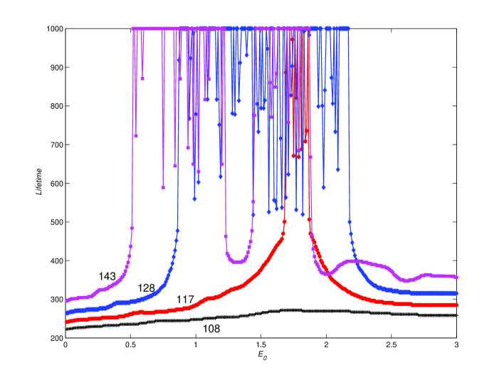
Figure 2: (Online version in colour.) Lifetimes of transients started from the Gaussian initial condition, for initial kinetic energies $0<E_{0}<3.0$ for $Re=108$ (black, $+$), $Re=117$ (red, $\circ$), $Re=128$ (blue, $\Diamond$) and $Re=143$ (magenta, $\Box$). Parameters are $\sigma=0.2$, $L_{x}=1.75\pi$, $L_{z}=1.2\pi$.

The overall impression of figure 2 is of a well defined transition from laminar to spatio-temporally complex dynamics for a range of initial perturbations. It is clear that windows of rapid attraction to the laminar state remain, for example for $Re=143$ and initial energies around $E_{0}=1.3$.

3.3 Transition boundary and structure of the chaotic saddle

The well defined ‘transition boundary’ at which there is an abrupt increase in lifetimes is shown clearly in figure 3 which presents a colour-coded surface plot of lifetimes as $Re$ and $E_{0}$ vary. In contrast to previous similar plots, for example figure 6 of Moehlis et al. (2004), and see also figure 11 in the present paper, where spatio-temporally complicated transients appear at around $Re=120$ at the ends of ‘wispy’ dendritic fingers that coalesce as $Re$ increases, figure 3 indicates the sudden appearance of a ‘fatter’ chaotic saddle in phase space.

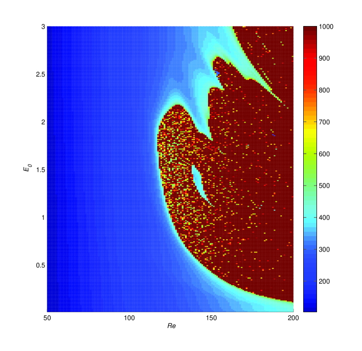
Figure 3: Lifetimes of transients started from the Gaussian initial condition, over the range $0<E_{0}<3.0$ and $50\leq Re\leq 200$. Parameters are $\sigma=0.2$, $L_{x}=1.75\pi$, $L_{z}=1.2\pi$.

The chaotic saddle appears to become less ‘porous’ as $Re$ increases, and there appears to be only one substantial hole, at around $Re=140$, $E_{0}=1.4$. As in Moehlis et al. (2004) we might anticipate that figure 3 has fine scale structure as we zoom in. In contrast to the results of that paper we find however that finer-scale investigations do not reveal any coherent organisation to the lifetimes: instead of regions of concentric bands of different colours, for example, we find merely fine-scale apparent randomness and intermittency.

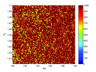
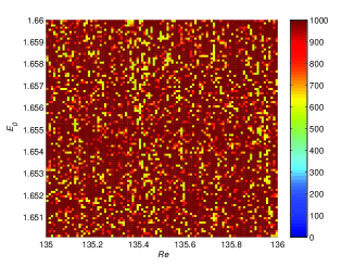
(a)                                                    (b)

Figure 4: (Online version in colour.) Enlargements of figure 3 showing a lack of coherent organisation to the lifetimes at higher resolution in $Re$ and $E_{0}$. (a) Transient lifetimes over the range $1.6<E_{0}<1.7$ and $130\leq Re\leq 140$. (b) Transient lifetimes over the range $1.65<E_{0}<1.66$ and $135\leq Re\leq 136$ as indicated by the black square in (a). For both figures, the other parameter values are $\sigma=0.2$, $L_{x}=1.75\pi$, $L_{z}=1.2\pi$.

This is illustrated in figure 4. Figure 4(a) shows the region $130\leq Re\leq 140$, $1.6\leq E_{0}\leq 1.7$ with a ten-fold increase in the resolution along each axis. Figure 4(b) shows a further order of magnitude increase in the resolution both in $Re$ and in $E_{0}$; this part of the figure corresponds to the region within the black box in the centre of figure 4(a). This very detailed enlargement appears to exhibit some slight correlation, for example a propensity to favour lifetimes of around 600 time units at $Re\approx 135.4$ but otherwise the unpredictable intermittent nature of the dynamics continues as we consider finer and finer divisions in $Re$ and $E_{0}$. This qualitative observation should be contrasted with the lifetimes figures plotted by Moehlis et al. (2004) which exhibit much more structure. We return to this point in section 3(3.6).

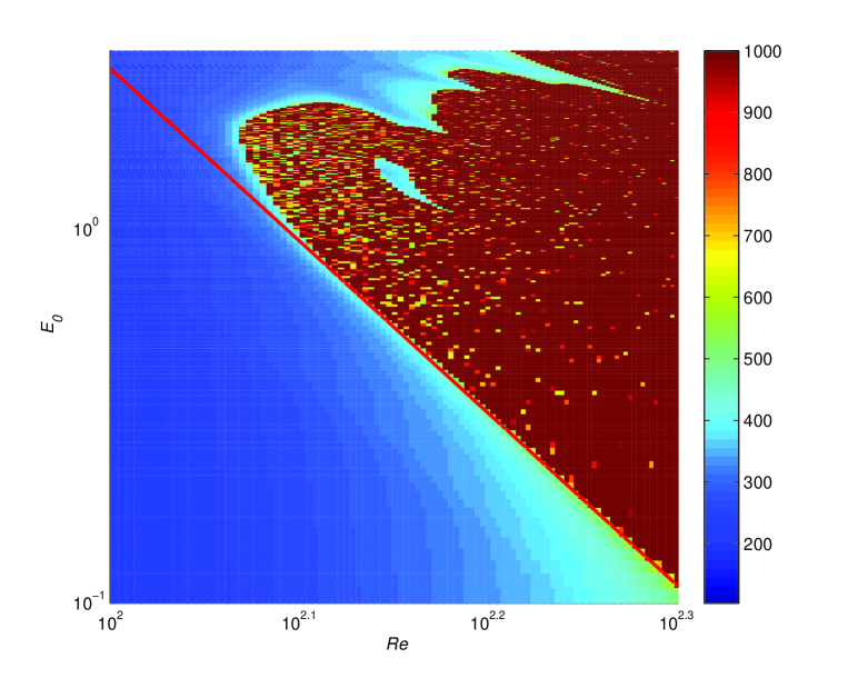
Figure 5: Log–log plot of transient lifetimes over the range $0.1<E<3.0$ and $100\leq Re\leq 200$ to show power law form of the lower boundary of the attractor. The solid (red) line indicates the power-law $E_{0}=\left(\frac{125}{Re}\right)^{4.65}$. Parameter values are $\sigma=0.2$, $L_{x}=1.75\pi$, $L_{z}=1.2\pi$.

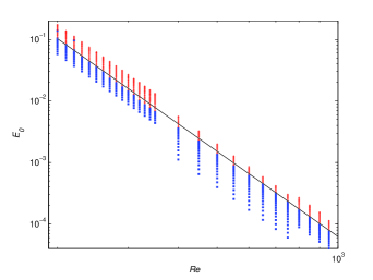
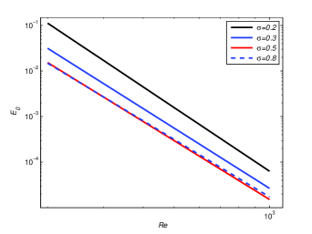
(a)                                                      (b)

Figure 6: (Online version in colour.) Estimates of the lower boundary of the chaotic saddle over the range $200<Re<1000$. (a) $\sigma=0.2$; squares (blue) indicate rapid return to the laminar state. ‘$+$’ symbols denote a long-lived chaotic transient. The black line indicates the power-law scaling of the lower boundary. (b) Best-fit power laws for a range of values of $\sigma$, showing a broad insensitivity to the width parameter. Parameter values are $L_{x}=1.75\pi$, $L_{z}=1.2\pi$.

The lower boundary of the chaotic saddle is of particular physical interest, since it describes the smallest amplitude perturbation required to produce an extended chaotic transient. For the particular form of perturbation used here, in the case $\sigma=0.2$, we find numerically that the lower boundary in figure 3 is remarkably well fitted by a power law curve as illustrated in the log-log plot in figure 5. Additional computations show that a power law continues to provide a very good fit as $Re$ is increased, up to at least $Re=10^{3}$, as shown in figure 6(a). The black curve in figure 6(a) is the best-fit curve

$$E_{0}=\left(\frac{122}{Re}\right)^{4.6}.$$ (28)

Blue squares in figure 6 indicate that the flow returned to laminar before the computational time limit $T_{\mathrm{max}}$ was reached, while red $+$ signs indicate that the flow did not relaminarise before $t=T_{\mathrm{max}}$. We set $T_{\mathrm{max}}=5000$ for $200<Re\leq 750$ and $T_{\mathrm{max}}=10000$ for $800\leq Re\leq 950$.

Table 2: Dependence of power-law scalings on the width $\sigma$ of initial condition.

$\sigma$	Constant, $c$	Exponent, $p$
$0.2$	$122$	$4.6$
$0.3$	$91.2$	$4.4$
$0.5$	$75.7$	$4.3$
$0.8$	$73.4$	$4.2$

In figure 6(b) we show the best-fit power-law for the boundary between laminar and spatio-temporally complicated flow for different widths of the Gaussian initial condition (24). All are excellent fits to the data over the range $200<Re<1000$, and the results are identical for computations using 128 modes or 32 modes in $z$. Since the slopes of the power-laws become more negative as the coefficient increases, the overall envelope of perturbation energies as $Re$ increases, formed by taking the minimum value over all four curves, has contributions from each curve at sufficiently large $Re$. This envelope is an estimate of the true lower boundary for which we would ideally compute the minimum over all possible forms of initial perturbation.

For perturbations with a Gaussian profile (24), and for the range of $\sigma$ considered here, it appears unlikely that the differences in exponents would be detectable experimentally over the range of relevant and accessible $Re$. Table 2 gives the details of the best-fit parameters of the power-laws shown in figure 6(b), using a functional form $E_{0}=(c/Re)^{p}$.

3.4 Lifetime distributions

Moehlis et al also computed the distribution of lifetimes of turbulent transients at fixed initial energies and Reynolds numbers. They found that the survival probability $P(T)$ that the solution had not decayed back to the laminar state after a time $T$ was distributed exponentially, with a mean lifetime that increased rapidly with $Re$ above the critical value at which the chaotic saddle appeared. Numerically, we construct a lifetime distribution by distributing the initial energy randomly across a subset of the modes. For our spatially-extended model there are two possible approaches to randomising the distribution of energy.

In the first approach, the total initial energy is distributed uniformly on a spherical energy shell. This can be achieved straightforwardly by modifying the expressions (25) - (27) for the normalisation coefficients by replacing $E_{0}$ with $4E_{0}\xi_{j}^{2}$ in the expression for coefficient $c_{j}$, where $j=3,\ldots,6$. The coordinates $\xi_{j}$ are those of points distributed at random over the unit sphere in $\mathbb{R}^{4}$ given by $\sum_{j=3}^{6}\xi_{j}^{2}=1$. We refer to this as randomising over the amplitudes of the perturbations.

In the second approach, the central position of each Gaussian perturbation $A_{j}$ is shifted randomly in $z$ away from the centre of the domain $L_{z}/2$, i.e. the values of the coefficients $c_{3},\ldots,c_{6}$ are left unchanged but the centre of the Gaussian in (24) is modified for each amplitude $A_{j}$. Since we employ periodic boundary conditions, the total energy in the perturbation is preserved. We refer to this procedure as randomising over the locations of the perturbations.

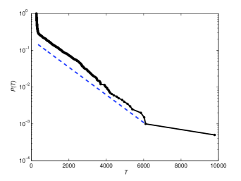
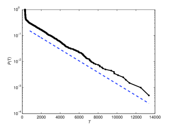
(a)                                                      (b)

Figure 7: (Online version in colour.) Distribution of lifetimes $P(T)$ computed over an ensemble of 2000 initial conditions produced by randomising over amplitudes of perturbations at $E_{0}=1.0$. (a) $Re=130$ (b) $Re=140$. Parameter values are $\sigma=0.2$, $L_{x}=1.75\pi$, $L_{z}=1.2\pi$.

Figure 7 shows the results of the first approach at two Reynolds numbers quite close to the transition boundary. At low lifetimes ($T<200$) the survival probability remains unity since any transient takes at least this finite amount of time to decay to within the prescribed threshold of the laminar state. As $T$ increases there is an initial sharp drop indicating that a substantial proportion of trajectories do decay rapidly, with lifetimes in the range $200<T<400$. At larger $T$ the distribution becomes close to a straight line on the linear-log plot, which is consistent with an exponential distribution $P(T)\sim a_{1}\exp(-a_{2}T)$ for $T\geq 400$ (approximately), as indicated by the dashed line. For $Re=130$ the best-fit coefficient values are $a_{1}=3.93\times 10^{-1}$ and $a_{2}=8.65\times 10^{-4}$. For $Re=140$ the best-fit coefficient values are $a_{1}=4.57\times 10^{-1}$, $a_{2}=5.11\times 10^{-4}$.

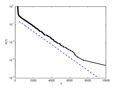
Figure 8: (Online version in colour.) Distribution of lifetimes $P(T)$ computed over an ensemble of 2000 initial conditions produced by randomising over the locations of perturbations at $E_{0}=1.0$ and $Re=130$. Parameter values are $\sigma=0.2$, $L_{x}=1.75\pi$, $L_{z}=1.2\pi$.

Similarly, figure 8 shows the lifetime distribution computed from the second approach, randomising over the locations of the perturbations. The distribution shows very similar characteristics to that in figure 7(a) and is again well-described by an exponential distribution with best-fit parameters $a_{1}=4.24\times 10^{-1}$ and $a_{2}=8.32\times 10^{-4}$. We observe that the values for the coefficient $a_{2}$ are very similar between the two randomisation methods. In all cases, we expect that as $Re$ increases the distribution exhibits systematic deviation from exponential and flattens out. We anticipate that, as in the ODE case, this is due to the appearance of stable attractors near the chaotic saddle, as $Re$ increases. These attracting sets then absorb trajectories with positive probability, leading to a proportion of trajectories which never return to the laminar state (Moehlis et al 2005).

3.5 Spanwise resolution

The very high resolution used in the $z$ direction ($N=128$ Fourier modes) is greater than required, for such a small domain, in order to capture the dynamics of the ‘active’ modes of the system. In order to probe the range of wavenumbers that make substantial contributions to the dynamics we investigated the effect of varying the truncation level of the numerical scheme in $z$. We define the ‘$m$-mode truncation’ of the PDEs (6) - (13) by keeping the Fourier modes $\sim\mathrm{e}^{\pm\mathrm{i}n\gamma z}$ for $0\leq n\leq m-2$ for $A_{1}$, $A_{4}$ and $A_{5}$, and keeping the modes for $0\leq n\leq m-1$ for $A_{2}$, $A_{3}$, $A_{6}$, $A_{7}$ and $A_{8}$. The $m$-mode truncation is thus a collection of (at most) $16m-14$ real ODEs. This is an upper bound on the effective dimension of the ODE dynamics since not every real and imaginary part is coupled for every $m$.

By construction, this further reduction resembles the Waleffe model in the particular case $m=2$, but by varying $m$ we are able to probe the influence of the higher-wavenumber modes on the location of the lower boundary for the onset of temporally complex dynamics. For each value of $E_{0}$ and $m$, a single initial condition was used. This initial condition was the projection of the Gaussian profiles described in section 3(a) onto the available Fourier modes in $z$. Results are shown in figure 9.

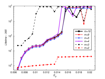
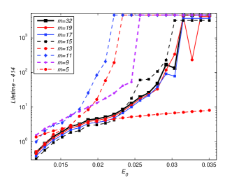
(a)                                                      (b)

Figure 9: (Online version in colour.) Lifetimes of transients $T$ as a function of initial energy $E_{0}$ for $Re=200$ in domains of widths (a) $L_{z}=1.2\pi$ and (b) $L_{z}=6\pi$, showing the effect of varying the truncation level $m$. Vertical axis is logarithmic for clarity, and shows the additional lifetime after subtracting a constant: $T-365$ in (a), $T-414$ in (b). In (a) the data for $m=9$ and $m=5$ lie exactly on the $m=16$ values: they are artificially offset vertically for clarity. In (b) the data for $m=19$, $m=17$ and $m=15$ lie exactly on the $m=32$ values and are similarly offset for clarity. Computations were terminated at $T_{\mathrm{max}}=5000$. Parameter values are $\sigma=0.8$, $L_{x}=1.75\pi$.

Figure 9(a), for the small domain $L_{z}=1.2\pi$, shows that computations with truncation levels $m\geq 5$ produce an identical indication of the boundary between laminar and spatio-temporally complex behaviour. The case $m=4$ is qualitatively but not quantitatively correct. For the larger domain $L_{z}=6\pi$, figure 9(b) indicates that the numerical results are essentially unchanged for $m\geq 17$. The number of Fourier modes required to maintain accuracy in the larger domain is therefore broadly in line with, although slightly lower than, what one might naively expect.

Finally we note that as $m$ decreases further, the boundary appears consistently to move to lower $E_{0}$. This behaviour is purely a function of the organisation of invariant sets in phase space; it is not clear that there is a physical reason why these should appear to move in one direction or the other.

3.6 Spatio-temporal dynamics and effect of initial conditions

In this final subsection we comment on the spatio-temporal dynamics of the PDEs for initial energies near the transition boundary, and we compare the results of section 3(c) for the lifetimes of transients with those in this section obtained using sinsoidal initial conditions. Figure 10 shows the spatial and temporal evolution of the PDEs for $Re=200$ and $E_{0}=0.11$, just above the transition boundary. The quantity $\tilde{E}(z,t)-A_{1}^{2}+(A_{1}-\sqrt{2})^{2}$ is plotted in the figure, so that the laminar state $A_{1}=\sqrt{2}$ is at level zero, where $\tilde{E}(z,t)$ is defined in (22). The initial monotonic decay towards the laminar state is interrupted by the growth of oscillatory disturbances. These disturbances generate a sharp spike in the kinetic energy, localised both in space and time, before the solution settles into a spatio-temporally chaotic state. For comparison, at $E_{0}=0.1$ we observe only monotonic decay to the laminar state.

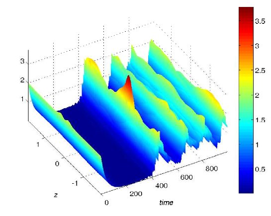
Figure 10: (Online version in colour.) Space-time plot of the local energy quantity $\tilde{E}(z,t)-A_{1}^{2}+(A_{1}-\sqrt{2})^{2}$, indicated by both surface height and colour, for the PDEs (6) - (13) for $Re=200$ in the minimal flow unit domain. $\tilde{E}(z,t)$ is defined in equation (22). The additional square terms shift the laminar state to the zero level in the plot and serve to highlight the localised ‘edge’ state at $t\approx 450$. Parameter values are $E_{0}=0.11$, $\sigma=0.2$, $L_{x}=1.75\pi$, $L_{z}=1.2\pi$.

Analysis of the energy distribution across Fourier modes shows that the small-scale oscillations just prior to the localised spike involve many higher-wavenumber Fourier modes. These mode amplitudes grow very rapidly as we approach the spike state. Since the formation of the spike is, in almost every case, the ‘edge state’ that is the precursor to spatio-temporally complicated dynamics, one interpretation of the results in the previous sub-section is that the spatial resolution required to correctly determine the boundary of the basin of attraction of the laminar state is indicated by the resolution required to describe accurately these spatially-localised spikes.

More generally, the dynamics near the boundary between monotonic relaminarisation and spatio-temporal complexity appear to depend on the evolution of high-wavenumber modes, seeded by the use of a Gaussian initial condition which injects energy into every available mode. This is in contrast with the sinusoidal initial conditions used in previous reduced models, where, by construction, such a sinusoidal initial condition was the only possible choice.

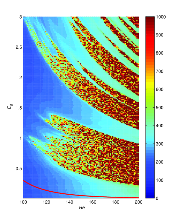
Figure 11: Lifetimes of transients started from the sinusoidal initial condition, over the range $0<E_{0}<3.0$ and $100\leq Re\leq 200$. Solid (red) line indicates the boundary $E_{0}=(75.7/Re)^{4.3}$ corresponding to the lowest of the boundaries in figure 6(b) for Gaussian perturbations. Parameter values are $L_{x}=1.75\pi$, $L_{z}=1.2\pi$. Computations used $N=32$ Fourier modes in $z$ and were terminated at $T_{\mathrm{max}}=1000$.

In figure 11 we show the analogous plot to figure 3 for the lifetimes of transients, but in this case using a sinusoidal initial condition instead of a Gaussian profile. For the sinusoidal initial condition we set $A_{2}=c_{2}\cos\gamma z$; $A_{3}=c_{3}\sin\gamma z$; $A_{4}=c_{4}$; $A_{5}=c_{5}$; $A_{1}=A_{6}=A_{7}=A_{8}=0$ where the constants $c_{2},\ldots,c_{5}$ are given by

$$c_{2}=\sqrt{\frac{\alpha E_{0}}{2\pi L_{z}}},\quad c_{3}=\sqrt{\frac{\alpha E_{0}}{(\beta^{2}+\gamma^{2})\pi L_{z}}},\quad c_{4}=\sqrt{\frac{E_{0}}{2\pi\alpha L_{z}}},\quad c_{5}=\sqrt{\frac{E_{0}}{\alpha\pi L_{z}}},$$

so that the inital kinetic energy $E_{0}$, defined in (22), is distributed equally between the four non-zero amplitudes.

Comparing figures 3 and 11 there are important qualitative and quantitative differences. Firstly, the boundary between relaminarisation and spatio-temporal complexity is much more obvious in figure 3 where we employ the Gaussian initial condition. The boundary in figure 11 shows much more ‘structure’; it is much less obvious that a boundary in the sense, for example, of a countable collection of (piecewise) continuous curves in the $(Re,E_{0})$ plane, can even be defined. Many deep valleys of short lifetimes persist up to $Re=200$ and beyond. Secondly, the solid (red) line in figure 11 shows the lowest boundary computed for Gaussian perturbations, corresponding to $\sigma=0.5$, see table 2. It appears that that the laminar state is substantially more sensitive to Gaussian perturbations than those of the same energy but in the form of low-wavenumber sinusoids. Tentatively, based only on the data in figure 11, we suggest that the lower boundary of the appearance of spatiotemporally complex dynamics arising from the sinusoidal perturbation scales as $E_{0}\sim Re^{-2}$, i.e. perturbation amplitude scaling as $Re^{-1}$. This is a typical exponent produced by very many reduced models of very low order, as summarised and discussed by Baggett & Trefethen (1997).

Within the region of spatio-temporally complex dynamics, the lifetimes in figure 11 and in additional enlargements (not shown here) show a degree of correlation between lifetimes at neighbouring points in the $(Re,E_{0})$ plane which is not nearly so clearly shown to exist in figure 3 or in the enlargements shown in figure 4.

In summary, in these respects figure 11 is reminiscent of lifetime plots for the very low-dimensional models of Moehlis et al (2004), see their figures 6 and 8, and figures 5 and 6 in the paper by Eckhardt & Mersmann (1999). We conclude that allowing for the accurate representation of spatially-localised initial conditions by extending the spanwise resolution of the model generates results that differ substantially, both qualitatively and quantitatively, from those of previous reduced models.

4 Discussion and conclusions

In this paper we have presented an extended version of the Galerkin-truncated model due to Waleffe (1997) for the transition to turbulence (or, at least, spatio-temporally complex dynamics) in sinusoidal shear flow. This model is appealing since it provides an intermediate step between previous analytical work and DNS of the full Navier–Stokes equations. Preserving full resolution in the spanwise ($z$) direction and removing the assumption of periodicity allows both the use of spatially-localised initial conditions, and the (transient) formation of localised structures in the flow which (although unstable) are known to exist and play a role in mediating the onset of turbulence. The use of a small number of Fourier modes in the wall-normal ($y$) and streamwise ($x$) directions provides the simplification of the underlying Navier–Stokes equations, which in turn allows us to perform very detailed investigations of the dynamics of this reduced model.

We compare our results with those of previous authors, in order to see which properties are common to these different approaches, and which are not. For example, we find, in agreement with the results of Moehlis et al 2004, that the lifetimes of turbulent transients are well-described by an exponential distribution. However, our results show that the transition boundary, while exhibiting some of the ‘structured’ shape observed by many authors (including, in the case of pipe flow, Schneider, Eckhardt & Yorke 2007), appears at lower perturbation energies, and much more abruptly, than for the ODE models investigated by Eckhardt & Mersmann (1999) and Moehlis et al (2004). The PDE model that we present here is able to represent both spatially-localised and spatially-extended initial conditions and therefore we are able to make direct comparisons of this kind.

Our key finding is that spatially-localised initial conditions are able to provoke complicated behaviour at substantially lower energies than the sinusoidal, spatially-extended perturbations used in previous studies. Moreover, the perturbation energy at the lower boundary of the chaotic saddle appears to scale as $Re^{p}$ with the exponent $p\approx-4.3$, rather than $Re^{-2}$ as in Eckhardt & Mersmann’s 19-mode truncated ODE model (note that their figure 5 showing an $Re^{-1}$ power law plots $Re$ against mode amplitude which is proportional to $E_{0}^{1/2}$). In the present work, the exponent in this power-law scaling was found to depend only weakly on the width of the Gaussian perturbation used.

In addition, our results are robust to the numerical resolution used in the spanwise direction, and, for a relatively small domain of width $L_{z}=1.2\pi$, point to the necessity of keeping around $5$ Fourier modes in $z$ in order accurately to capture the dynamics of the fully-resolved PDE model. One possible explanation of these results is that admitting higher-wavenumber modes generates many more invariant sets within the boundary of the basin of attraction of the laminar state. Then, even small amounts of initial energy in these modes forces the system to spend much longer in the vicinity of these sets before being able to relaminarise. In this sense, ‘holes’ in the basin boundary are filled in. The existence of these new invariant sets, and the lack of ‘holes’, leads to a robustness in the lengths of transients, and therefore to a more clearly defined boundary between monotonic relaminarisation and longer-lived transients.

It would clearly be of interest in future work to look at the relation between localised states which have been observed and studied in some detail in DNS for shear flow problems (Schneider et al 2010a, 2010b) and the dynamics of the reduced model presented here. We anticipate that the reduced model contains such states, and the homoclinic snaking bifurcation diagrams that typically organise them in driven dissipative systems such as shear flows, just as model ODE truncations, for example that discussed in Moehlis et al 2005, contain equilibria and time-periodic solutions very similar to those located in DNS (Nagata 1990; Gibson et al 2009). It should be possible systematically to further reduce the model equations presented here in order to make direct connections between theoretical work on localised states (Burke & Knobloch 2006; Chapman & Kozyreff 2009; Dawes 2010) and the DNS results referred to above. In turn, the identification and analysis of additional unstable invariant sets within the boundary of the basin of attraction of the laminar state (as discussed by Lebovitz 2009), and their parameter dependence, will greatly help our understanding of the process of relaminarisation.

- [1]
- [2] Baggett, J.S. & Trefethen, L.N. 1997 Low-dimensional models of subcritical transition to turbulence. Phs. Fluids 9, 1043–1053
- [3]
- [4] Barkley, D. & Tuckerman, L.S. 2007 Mean flow of turbulent-laminar patterns in plane Couette flow. J. Fluid Mech. 576, 109–137
- [5]
- [6] Burke, J. & Knobloch, E. 2006 Localized states in the generalized Swift–Hohenberg equation. Phys. Rev. E 73, 056211.
- [7]
- [8] Chapman, S. J. & Kozyreff, G. 2009 Exponential asymptotics of localized patterns and snaking bifurcation diagrams. Physica D 238, 319–354.
- [9]
- [10] Cox, S.M. & Matthews, P.C. 2002 Exponential time differencing for stiff systems. J. Comp. Phys. 176, 430–455
- [11]
- [12] Dawes, J.H.P. 2010 The emergence of a coherent structure for coherent structures: localized states in nonlinear systems. Phil. Trans. R. Soc. A 368, 3519–3534
- [13]
- [14] Drazin, P.G. & Reid, W.H. 1981 Hydrodynamic Stability. CUP, Cambridge.
- [15]
- [16] Duguet, Y., Schlatter P. & Henningson D.S. 2009 Localized edge states in plane Couette flow. Phys. Fluids 21, 111701
- [17]
- [18] Eckhardt, B., & Mersmann, A. 1999 Transition to turbulence in a shear flow. Phys. Rev. E 60, 509–517
- [19]
- [20] Hamilton, J.M., Kim, J. & Waleffe, F. 1995 Regeneration mechanisms of near-wall turbulence structures. J. Fluid Mech. 287, 317–348
- [21]
- [22] Gibson, J.F., Halcrow, J. & Cvitanovic, P. 2009 Equilibrium and traveling-wave solutions of plane Couette flow. J. Fluid Mech. 638, 1–24
- [23]
- [24] Kerswell, R. 2005 Recent progress in understanding the transition to turbulence in a pipe. Nonlinearity 18, R17–R44
- [25]
- [26] Lagha, M. & Manneville, P. 2007 Modeling transitional plane Couette flow. Eur. Phys. J. B 58, 433–447
- [27]
- [28] Lebovitz, N.R. 2009 Shear-flow transition: the basin boundary Nonlinearity 22, 2645–2655
- [29]
- [30] Lorenz, E.N. 1963 Deterministic nonperiodic flow. J. Atmos. Sci. 20, 130-141
- [31]
- [32] Manneville P., & Locher F. 2000 A model for transitional plane Couette flow. C. R. Acad. Sci. Paris 328, 159–164
- [33]
- [34] Manneville, P. 2004 Spots and turbulent domains in a model of transitional plane Couette flow. Theor. Comp. Fluid Dyn. 18, 169–181
- [35]
- [36] Moehlis, J., Faisst, H. & Eckhardt, B. 2004 A low-dimensional model for turbulent shear flows. New J. Phys. 6, 56
- [37]
- [38] Moehlis, J., Faisst, H. & Eckhardt, B. 2005 Periodic orbits and chaotic sets in a low-dimensional model for shear flows. SIAM J. Appl. Dyn. Syst. 4, 352
- [39]
- [40] Nagata, W. 1990 Three-dimensional finite-amplitude solutions in plane Couette flow: bifurcation from infinity. J. Fluid Mech. 217, 519
- [41]
- [42] Schneider, T.M., Eckhardt, B. & Yorke, J.A. 2007 Turbulent transition and the edge of chaos in pipe flow. Phys. Rev. Lett. 99, 034502
- [43]
- [44] Schneider, T.M., Marinc, D. & Eckhardt, B. 2009 Localization in plane Couette edge dynamics. In Advances in turbulence XII (ed. B. Eckhardt), pp. 83 85. Springer Proceedings in Physics, vol. 132. Berlin, Germany: Springer.
- [45]
- [46] Schneider, T.M., Marinc, D. & Eckhardt, B. 2010a Localized edge states nucleate turbulence in extended plane Couette cells. J. Fluid Mech. 646, 441–451.
- [47]
- [48] Schneider, T.M., Gibson, J.F. & Burke, J. 2010b Snakes and ladders: localized solutions of plane Couette flow. Phys. Rev. Lett. 104, 104501
- [49]
- [50] Waleffe, F. 1997 On a self-sustaining process in shear flows. Phys. Fluids 9, 883–900
- [51]
- [52] Willis, A.P. & Kerswell, R.R. 2009 Turbulent dynamics of pipe flow captured in a reduced model: puff relaminarization and localized ‘edge’ states. J. Fluid Mech. 619, 213–233
- [53]