Top-BESS model and its phenomenology

Abstract

We introduce the top-BESS model which is the effective description of the strong electroweak symmetry breaking with a single new $SU(2)_{L+R}$ triplet vector resonance. The model is a modification of the BESS model in the fermion sector. The triplet couples to the third generation of quarks only. This approach reflects a possible extraordinary role of the top quark in the mechanism of electroweak symmetry breaking. The low-energy limits on the model parameters found provide hope for finding sizable signals in the LHC Drell-Yan processes as well as in the s-channel production processes at the ILC. However, there are regions of the model parameter space where the interplay of the direct and indirect fermion couplings can hide the resonance peak in a scattering process even though the resonance exists and couples directly to top and bottom quarks.

I Introduction

Despite the great success of the Standard model (SM) GWS one essential component of the theory remains a puzzle: it is the actual mechanism behind the electroweak symmetry breaking (ESB). Spontaneous breaking of electroweak symmetry accompanied by the Higgs mechanism is the way to reconcile the massive gauge bosons with the principle of gauge invariance. The introduction of the Higgs complex doublet scalar field of a non-zero vacuum expectation value to the electroweak theory serves as a benchmark hypothesis for the mechanism. A direct consequence of this hypothesis is the presence of the scalar Higgs boson in the particle spectrum of the SM, not observed as of yet, though.

Nevertheless, there is a host of candidates for alternative extensions of the SM that offer their own mechanisms of ESB. If the Large Hadron Collider (LHC) does not discover the SM Higgs boson, ESB could originate from strongly interacting new physics. In this scenario the symmetry breaking is triggered by new non-perturbative forces which form bound states of new elementary particles. The bound states would appear in the particle spectrum as new resonances. Typical representatives of this scenario are the Technicolor model (TC) TC and its extensions ETC ; WalkingTC ; TopcolorTC .

More recent extra-dimensional theories ExtraDim predict the Kaluza-Klein towers of new resonances of which the lowest lying resonances might be discovered at the LHC. The attractiveness of this development is strengthened by Maldacena’s conjecture Maldacena on the dual-description relation between the extra-dimensional weakly interacting theories and the strongly interacting models in four dimensions.

Obviously, all the alternative extensions must converge to the SM without Higgs when pre-LHC energies are considered. Facing this plethora of hypotheses it is desirable to develop unifying descriptions of their low-energy phenomenologies. For this purpose, the formalism of effective Lagrangians is very suitable. The effective Lagrangians can accommodate new particles predicted by the extensions. The new particles are not only a by-product of a particular ESB mechanism but they will be needed to tame the model’s unitarity if the Higgs boson below 1 TeV is not found LeeQuiggThacker77 .

In this paper we introduce the top-BESS model (tBESS) — the modified version of the BESS (Breaking Electroweak Symmetry Strongly) model BESS . The basic ideas of the tBESS model were formulated already in tBESSActaPhysicaSlovaca . Both models describe a new $SU(2)$ vector boson triplet that can represent the spin-1 bound states of hypothetical new strong interactions. They are effective descriptions of strong Higgsless ESB based on the $SU(2)_{L}\times SU(2)_{R}\times U(1)_{B-L}\times SU(2)_{HLS}$ global symmetry of which the $SU(2)_{L}\times U(1)_{Y}\times SU(2)_{HLS}$ subgroup is also a local symmetry. “HLS” stands for the hidden local symmetry HLS , which is an auxiliary gauge symmetry introduced to accommodate the $SU(2)$ triplet of vector resonances. Beside the triplet, the models contain only the observed SM particles.

The BESS and tBESS models are gauge equivalent to the nonlinear sigma model on the $SU(2)_{L}\times SU(2)_{R}/SU(2)_{L+R}$ coset space with the $SU(2)_{L+R}$ vector triplet added in the way introduced by Weinberg WeinbergRho .

The BESS model also corresponds to the simplest version of the five-dimensional Higgsless model in the deconstructed picture of three lattice sites and the $SU(2)_{L}\times SU(2)\times U(1)_{Y}$ gauge symmetry, when direct couplings between SM fermions and new vector bosons are introduced 3siteExtraDimBESS . The four-site Higgsless model based on the $SU(2)_{L}\times SU(2)_{1}\times SU(2)_{2}\times U(1)_{Y}$ gauge symmetry 4siteExtraDimDBESS corresponds to the degenerated BESS model DBESS .

In the tBESS model we modify the direct interactions of the vector triplet with fermions. While in the BESS model there is a universal direct coupling of the triplet to all fermions of a given chirality, in our modification we admit direct couplings of the new triplet-to-top and bottom quarks only. Our modification is inspired by the speculations about a special role of the top quark (or the third quark generation) in the mechanism of ESB  snowmass ; Han4 . The large top mass is surprisingly close to the ESB scale: $m_{t}\approx v/\sqrt{2}$. This suggests that $m_{t}$ could be generated by the same mechanism as $M_{W}$ and $M_{Z}$, i.e., by the same strong interactions which are also responsible for ESB. If this were the case, we would expect the new triplet to couple significantly to the weak gauge bosons as well as to the top quark. This happens, for example, for the vector $\rho_{T}$ resonance of the Extended Technicolor ETC .

On the other hand, the mechanism behind the top mass could differ from the ESB mechanism. Thus, it can be represented by yet another sector of new strong interactions introduced just for that sake, e.g. the Topcolor of the Topcolor Assisted Technicolor TopcolorTC , where $\rho_{T}$ couples only weakly to the top quark. The neutral component of the new vector triplet can also mimic couplings of a $Z^{\prime}$ spin-1 resonance Han3 ; He which has large couplings to the top and bottom, vanishing couplings to $W$, $Z$, and very small couplings to fermions of the first two generations. The authors of Han1 ; Han2 ; Han3 studied the effective description of the situation when the third quark generation couples extraordinarily to the new strong resonances, scalar and vector ones, under some simplifying assumptions. They also studied various processes as probes of the resonances.

In the tBESS model, we take the possible chirality dependence of the triplet-to-top/bottom coupling into account multiplying the $SU(2)_{HLS}$ gauge coupling $g^{\prime\prime}$ by the $b_{L}$ and $b_{R}$ parameters for the left and right fermion doublets, respectively. In addition, we can disentangle the triplet-to-top-quark right coupling from the triplet-to-bottom-quark right coupling. This breaks the $SU(2)_{R}$ symmetry which is broken by the SM interactions, anyway. For this sake, we have introduced a free parameter, $0\leq p\leq 1$. The $p$ parameter can weaken the strength of the triplet-to-bottom-quark right coupling. However, the $SU(2)_{L}$ symmetry does not allow us to do the same splitting for the left quark doublet.

There are two more invariant terms introduced in the tBESS effective Lagrangian when compared to the BESS model. They are multiplied by additional free parameters, $\lambda_{L}$ and $\lambda_{R}$. While the $\lambda$ terms do not have a significant impact on the behavior of the model at energies around the mass of the vector triplet, they do influence the low-energy limits for its parameters. Namely, the presence of $\lambda$ terms helps to relax the low-energy limits for the fermion parameters.

In the tBESS model the vector triplet is introduced as a gauge field which results in the mixing of the triplet with the electroweak gauge bosons. Consequently, the indirect — mixing-induced — interactions of the vector triplet with fermions appear on the scene. For the light fermions this is the only way they can interact with the vector triplet in the tBESS model. Of course, the interactions are suppressed by the elements of the mixing matrix.

Since the indirect couplings are suppressed by the mixing factors it does not have to seem worthwhile to study the tBESS model in processes where the vector resonances couple to light fermions. We suggest that despite this naive expectation it is not necessarily so.

There are regions of the parameter space where the interference of the direct and indirect couplings suppresses or even zeros a particular top/bottom decay channel of the vector triplet. Consequently, the resonance peak might not be visible in a particular experiment even though the new vector triplet exists.

This paper is organized as follows. In Section II we introduce the tBESS effective Lagrangian. While Subsection II.1 recalls the details of the gauge boson and ESB sectors that are shared with the BESS model, in Subsection II.2 our modifications of the fermion sector are explained. In Section III the basic properties of the tBESS model are discussed. Beside the vector resonance decay widths, the unitarity and low-energy limits for the model are derived in Subsections III.2 and III.3, respectively. In Subsection III.4 the effect of suppressing the partial decay widths of the vector triplet for some values of the parameter space is discussed. In Subsection III.5 we illustrate the impact of the suppression on $e^{+}e^{-}$ processes. We also suggest that it might be feasible to use the light fermion enabled processes at the ILC and the LHC (Drell-Yan) to study the tBESS model. Section IV contains our conclusions followed by appendices.

II The top-BESS model

The top-BESS effective Lagrangian can be split in three parts

$${\cal L}_{tBESS}={\cal L}_{GB}+{\cal L}_{ESB}+{\cal L}_{ferm},$$ (1)

where ${\cal L}_{GB}$ describes the gauge-boson sector including the $SU(2)_{HLS}$ triplet, ${\cal L}_{ESB}$ is the scalar sector responsible for spontaneous breaking of the electroweak and hidden local symmetries, and ${\cal L}_{ferm}$ is the fermion Lagrangian of the model. The individual terms will be elaborated on in the subsections below. Of course, the SM Lagrangian, up to the Higgs doublet, must be a low-energy approximation of ${\cal L}_{tBESS}$.

II.1 The $SU(2)_{HLS}$ vector triplet Lagrangian

We start with reviewing the gauge-field and scalar sectors of the tBESS model which are — except for the used notations — identical with those of the original BESS model BESS . It contains six unphysical real scalar fields, would-be Goldstone bosons of the model’s spontaneous symmetry breaking. Thus, naturally, the sector provides the energy scale $v$ of ESB.

Beside the SM gauge fields $W_{\mu}^{a}(x)$ and $B_{\mu}(x)$ there is the $SU(2)_{HLS}$ gauge triplet $\vec{V}_{\mu}=(V_{\mu}^{1},V_{\mu}^{2},V_{\mu}^{3})$ introduced in the model. Under the $\Gamma^{glob}\times SU(2)_{HLS}^{loc}$ group, where $\Gamma=SU(2)_{L}\times SU(2)_{R}$, it transforms as

$$\mbox{\boldmath$V$}_{\mu}\rightarrow h^{\dagger}\mbox{\boldmath$V$}_{\mu}h+h^{\dagger}\partial_{\mu}h,$$ (2)

where $h(x)\in SU(2)_{HLS}^{loc}$ and $\mbox{\boldmath$V$}_{\mu}=i\frac{g^{\prime\prime}}{2}V_{\mu}^{a}\tau^{a}$. The $2\times 2$ matrices $\vec{\tau}=(\tau^{1},\tau^{2},\tau^{3})$ are the $SU(2)$ generators.

The gauge-boson Lagrangian ${\cal L}_{GB}$ is composed of the Lagrangians for the individual gauge bosons

$${\cal L}_{GB} = {\cal L}_{W}+{\cal L}_{B}+{\cal L}_{V},$$ (3)

$${\cal L}_{W} = \frac{1}{2g^{2}}\mbox{Tr}(\mbox{\boldmath$W$}_{\mu\nu}\mbox{\boldmath$W$}^{\mu\nu}),$$ (4)

$${\cal L}_{B} = \frac{1}{2g^{\prime 2}}\mbox{Tr}(\mbox{\boldmath$B$}_{\mu\nu}\mbox{\boldmath$B$}^{\mu\nu}),$$ (5)

$${\cal L}_{V} = \frac{2}{g^{\prime\prime 2}}\mbox{Tr}(\mbox{\boldmath$V$}_{\mu\nu}\mbox{\boldmath$V$}^{\mu\nu}),$$ (6)

with the field strength tensors

$$\mbox{\boldmath$W$}_{\mu\nu} = \partial_{\mu}\mbox{\boldmath$W$}_{\nu}-\partial_{\nu}\mbox{\boldmath$W$}_{\mu}+\mbox{$[$}\mbox{\boldmath$W$}_{\mu},\mbox{\boldmath$W$}_{\nu}\mbox{$]$},$$ (7)

$$\mbox{\boldmath$B$}_{\mu\nu} = \partial_{\mu}\mbox{\boldmath$B$}_{\nu}-\partial_{\nu}\mbox{\boldmath$B$}_{\mu},$$ (8)

$$\mbox{\boldmath$V$}_{\mu\nu} = \partial_{\mu}\mbox{\boldmath$V$}_{\nu}-\partial_{\nu}\mbox{\boldmath$V$}_{\mu}+\mbox{$[$}\mbox{\boldmath$V$}_{\mu},\mbox{\boldmath$V$}_{\nu}\mbox{$]$},$$ (9)

where $\mbox{\boldmath$W$}_{\mu}=igW_{\mu}^{a}\tau^{a}$, $\mbox{\boldmath$B$}_{\mu}=ig^{\prime}B_{\mu}Y$ are $SU(2)_{L}$ and $U(1)_{Y}$ gauge fields.

To generate the gauge-boson masses, the six real scalar fields $\varphi_{L}^{a}(x),\varphi_{R}^{a}(x),\;a=1,2,3$, are introduced as parameters of the $\Gamma$ group elements in the exp form

$$\Xi(\vec{\varphi}_{L},\vec{\varphi}_{R})=\mbox{diag}(\;\xi(\vec{\varphi}_{L}),\;\xi(\vec{\varphi}_{R})\;)\;\;\in\;\Gamma,$$ (10)

where $\vec{\varphi}=(\varphi^{1},\varphi^{2},\varphi^{3})$, $\xi(\vec{\varphi})=\exp(i\vec{\varphi}\vec{\tau}/v)\in SU(2)$ and $v$ is the scale of ESB. The $\Xi$ matrix transforms linearly under $\Gamma^{glob}\times SU(2)_{HLS}^{loc}$:

$$\Xi(\vec{\varphi}_{L},\vec{\varphi}_{R})\;\;\rightarrow\;\;G\cdot\Xi\cdot H(x),$$ (11)

where $G=\mbox{diag}(g_{L},g_{R})$, $H(x)=\mbox{diag}(h(x),h(x))$, $g_{L,R}\in SU(2)_{L,R}$, $h\in SU(2)_{HLS}$. The scalar fields couple to the gauge bosons in the form given by the $[SU(2)_{L}\times U(1)_{Y}\times SU(2)_{HLS}]^{loc}$ invariant Lagrangian

$${\cal L}_{ESB}=-\frac{v^{2}}{2}\left[\mbox{Tr}\left(\bar{\Omega}_{\mu}^{\perp}\right)^{2}+\alpha\mbox{Tr}\left(\bar{\Omega}_{\mu}^{\parallel}\right)^{2}\right],$$ (12)

where $\alpha$ is a free parameter and $\bar{\Omega}_{\mu}^{\perp}$ and $\bar{\Omega}_{\mu}^{\parallel}$ are $SU(2)_{L-R}$ and $SU(2)_{L+R}$ projections of the gauged Maurer-Cartan 1-form $\bar{\Omega}_{\mu}$

$$\bar{\Omega}_{\mu}(\vec{\varphi}_{L},\vec{\varphi}_{R}) = \Xi^{\dagger}(\vec{\varphi}_{L},\vec{\varphi}_{R})\cdot D_{\mu}\Xi(\vec{\varphi}_{L},\vec{\varphi}_{R}),$$ (13)

$$\bar{\Omega}^{\parallel,\perp}_{\mu}(\vec{\varphi}_{L},\vec{\varphi}_{R}) = \frac{1}{2}\left[\bar{\Omega}_{\mu}(\vec{\varphi}_{L},\vec{\varphi}_{R})\pm\bar{\Omega}_{\mu}(\vec{\varphi}_{R},\vec{\varphi}_{L})\right].$$ (14)

The projections have a block-diagonal form

$$\bar{\Omega}^{\parallel,\perp}_{\mu}=\mbox{diag}(\bar{\omega}^{\parallel,\perp}_{\mu},\pm\bar{\omega}^{\parallel,\perp}_{\mu}),$$ (15)

where the expressions for $\bar{\omega}^{\parallel,\perp}_{\mu}$ in terms of $\xi$’s can be inferred from Eqs. (10), (13), and (14). The covariant derivative $D_{\mu}\Xi$ reads

$$D_{\mu}\Xi(\vec{\varphi}_{L},\vec{\varphi}_{R})\;=\;\partial_{\mu}\Xi\;+\;\mbox{\boldmath$X$}_{\mu}\cdot\Xi\;-\;\Xi\cdot\mbox{\boldmath$V$}_{\mu},$$ (16)

where $\mbox{\boldmath$X$}_{\mu}=igW_{\mu}^{a}T_{L}^{a}+ig^{\prime}B_{\mu}Y$, $\mbox{\boldmath$V$}_{\mu}=i\frac{g^{\prime\prime}}{2}V_{\mu}^{a}T^{a}$, $T_{L}^{a}=\mbox{diag}(\tau^{a},0)$, $T_{R}^{3}=\mbox{diag}(0,\tau^{3})$, $T^{a}=\mbox{diag}(\tau^{a},\tau^{a})$, $Y=T_{R}^{3}+\frac{1}{2}(B-L)\mbox{\bf I}^{(4)}$, $\mbox{\bf I}^{(4)}=\mbox{diag}(1,1,1,1)$, and $B$, $L$ denote the baryon and lepton numbers, respectively.

It can be shown that all the six scalar fields can be transformed away by an appropriate gauge transformation. Thus they are unphysical. Namely, the scalar triplet $\vec{\sigma}=(\vec{\varphi}_{L}+\vec{\varphi}_{R})/2$ can be gauged away by the $SU(2)_{HLS}^{loc}$ transformation $h(x)=\xi(\vec{\sigma})$, leaving us with the pseudoscalar triplet $\vec{\pi}=(\vec{\varphi}_{L}-\vec{\varphi}_{R})/2$. The gauge transformation turns the Lagrangian (12) into the gauged nonlinear sigma model on the $SU(2)_{L}\times SU(2)_{R}/SU(2)_{L+R}$ coset space. The triplet $\vec{\pi}$ plays a role of the Goldstone bosons which supply masses to the electroweak gauge bosons through the Higgs mechanism. The $SU(2)_{HLS}$ vector triplet enters the resulting nonlinear sigma model Lagrangian in the way introduced originally by Weinberg WeinbergRho .

To obtain the masses of the electroweak gauge bosons as well as of the new vector resonances their mass matrix has to be diagonalized. The eigenstate transformation matrices of the neutral and charged gauge-boson sectors, $O^{N}$ and $O^{C}$, transform the mass eigenstates to the flavor eigenstates

$$\left(\begin{array}[]{c}W^{3}\\ B\\ V^{3}\end{array}\right)_{flavor}=O^{N}\left(\begin{array}[]{c}A\\ Z\\ V^{0}\end{array}\right)_{mass},\;$$ (17)

$$\left(\begin{array}[]{c}W^{\pm}\\ V^{\pm}\end{array}\right)_{flavor}=O^{C}\left(\begin{array}[]{c}W^{\pm}\\ V^{\pm}\end{array}\right)_{mass}.$$ (18)

Note that $X^{\pm}=(X^{1}\mp iX^{2})/\sqrt{2}$ where $X=W,V$. In the limit $M_{W^{\pm}},M_{Z}\ll M_{V^{0}}$ which is equivalent to the condition $g\ll\sqrt{\alpha}g^{\prime\prime}$, the mixing matrices read

$$O^{N}=\left(\begin{array}[]{ccc}g^{\prime}/G&g/G&-g/g^{\prime\prime}\\ g/G&-g^{\prime}/G&-g^{\prime}/g^{\prime\prime}\\ 2\frac{gg^{\prime}}{Gg^{\prime\prime}}&\frac{g^{2}-g^{\prime 2}}{Gg^{\prime\prime}}&1\end{array}\right),$$ (19)

$$O^{C}=\left(\begin{array}[]{cc}1&-g/g^{\prime\prime}\\ g/g^{\prime\prime}&1\end{array}\right),$$ (20)

where $G=\sqrt{g^{2}+g^{\prime 2}}$. In the same limit the gauge masses can be approximated by the following formulas:

$$M_{W^{\pm}} = \frac{vg}{2}\left(1-\frac{g^{2}}{2g^{\prime\prime 2}}\right),$$ (21)

$$M_{Z} = \frac{vG}{2}\left[1-\frac{(g^{2}-g^{\prime 2})^{2}}{2g^{\prime\prime 2}G^{2}}\right],$$ (22)

$$M_{V^{\pm}} = \frac{\sqrt{\alpha}vg^{\prime\prime}}{2}\left(1+\frac{g^{2}}{2g^{\prime\prime 2}}\right),$$ (23)

$$M_{V^{0}} = \frac{\sqrt{\alpha}vg^{\prime\prime}}{2}\left(1+\frac{G^{2}}{2g^{\prime\prime 2}}\right).$$ (24)

Of course, the mass of the photon $A$ is zero.

II.2 Fermion Lagrangian

In our approach, we modify the interactions of the new vector triplet with fermions. No new fermions beyond the SM have been introduced in the model. The modification singles out the new physics role of the third quark generation, and of the top quark in particular. Hence, we call the obtained effective Lagrangian the top-BESS model, or tBESS in short. It can be split in two parts

$${\cal L}_{ferm}={\cal L}_{ferm}^{SM}+{\cal L}_{(t,b)}^{tBESS},$$ (25)

where ${\cal L}_{ferm}^{SM}$ is the SM part of the fermion Lagrangian and ${\cal L}_{(t,b)}^{tBESS}$ contains the modification concerning the third quark generation.

The fermions are grouped into six $SU(2)_{L}$ doublets and six $SU(2)_{R}$ doublets $\psi_{h}^{a},a=1,\ldots,6$ where $h=L,R$ denotes the chirality of the fields. Under $\Gamma^{glob}\times SU(2)_{HLS}^{loc}$

$$\psi_{L,R}^{a}\;\;\rightarrow\;\;g_{L,R}\;\psi_{L,R}^{a},\;\;\;g_{L,R}\in SU(2)_{L,R}.$$ (26)

The leptonic and light quark doublets are indexed by the $a=1,\ldots,5$ range, $a=6$ is reserved for the top-bottom doublet. The useful construct for building the fermion Lagrangian is the matrix

$$\chi_{h}^{a}\equiv\chi(\vec{\varphi}_{h},\psi_{h}^{a})=\xi^{\dagger}(\vec{\varphi}_{h})\cdot\psi_{h}^{a}.$$ (27)

Under $\Gamma^{glob}\times SU(2)_{HLS}^{loc}$ it transforms as

$$\chi_{L,R}^{a}\;\;\rightarrow\;\;h^{\dagger}(x)\cdot\chi_{L,R}^{a},\;\;\;h(x)\in SU(2)_{HLS}^{loc}.$$ (28)

The $[\Gamma\times U(1)_{B-L}]^{glob}\times SU(2)_{HLS}^{loc}$ invariant Higgsless effective Lagrangian describing the SM physics of the fermion doublets reads

$${\cal L}_{ferm}^{SM}=\sum_{a=1}^{6}\left[I_{c}^{L}(\psi_{L}^{a})+I_{c}^{R}(\psi_{R}^{a})-I_{mass}(\psi^{a})\right],$$ (29)

where

$$I_{c}^{L}(\psi_{L}^{a}) = i\bar{\psi}_{L}^{a}(\!\not{\!\mbox{\boldmath$\partial$}}+\!\not{\!\!\mbox{\boldmath$W$}}+\!\not{\!\!\mbox{\boldmath$B$}})\psi_{L}^{a},$$ (30)

$$I_{c}^{R}(\psi_{R}^{a}) = i\bar{\psi}_{R}^{a}(\!\not{\!\mbox{\boldmath$\partial$}}+\!\not{\!\!\mbox{\boldmath$B$}})\psi_{R}^{a},$$ (31)

and

$$I_{mass}(\psi^{a})=\bar{\psi}_{L}^{a}UM_{f}\psi_{R}^{a}+\mbox{h.c.},$$ (32)

where $M_{f}$ is a $2\times 2$ diagonal matrix with the masses of the upper and bottom fermion doublet components on its diagonal and $U=\xi(\vec{\pi})\cdot\xi(\vec{\pi})=\exp(2i\vec{\pi}\vec{\tau}/v)$. Note that while $I_{c}^{L}$ and $I_{c}^{R}$ are invariants of $[\Gamma\times U(1)_{B-L}]^{glob}\times SU(2)_{HLS}^{loc}$ as well as of $[SU(2)_{L}\times U(1)_{Y}]^{loc}$, the $I_{mass}$ terms break $SU(2)_{R}\rightarrow U(1)_{R3}$.

The additional $[\Gamma\times U(1)_{B-L}]^{glob}\times SU(2)_{HLS}^{loc}$ and $[SU(2)_{L}\times U(1)_{Y}]^{loc}$ invariants read ($h=L,R$)

$$I_{b}^{h}(\psi_{h})=i\bar{\chi}_{h}\left[\!\not{\!\mbox{\boldmath$\partial$}}+\!\not{\!\mbox{\boldmath$V$}}+ig^{\prime}\!\not{\!\!B}(B-L)/2\right]\chi_{h},$$ (33)

and

$$I_{\lambda}^{h}(\psi_{h}) = i\bar{\chi}_{h}\!\not{\!\!\bar{\omega}}^{\perp}\chi_{h}$$ (34)

$$= i\bar{\chi}_{h}\left[\;\!\not{\!\!\omega}^{\perp}+(\xi_{L}^{\dagger}\!\not{\!\!\mbox{\boldmath$W$}}\xi_{L}-\xi_{R}^{\dagger}\!\not{\!\!\mbox{\boldmath$B$}}^{R3}\xi_{R})/2\right]\chi_{h},\;\;\;\;\;\;$$

where $\!\not{\!\!\mbox{\boldmath$B$}}^{R3}=ig^{\prime}\!\not{\!\!B}\tau^{3}$, and $\;\!\not{\!\!\omega}^{\perp}=(\xi_{L}^{\dagger}\!\not{\!\partial}\xi_{L}-\xi_{R}^{\dagger}\!\not{\!\partial}\xi_{R})/2$. Note that the $I_{b}^{h}$ terms contain the direct interactions of the vector triplet with fermions as opposed to the $\lambda$ invariants where there is no such interaction. However, the $\lambda$ terms do modify the couplings of the electroweak gauge bosons with fermions. The $\lambda$ terms were not present in the original BESS formulation BESS . Even though their values do not have a significant impact on the observed signals at the triplet peaks, they do influence the low-energy limits for the fermion parameters.

We use the invariants (33) and (34) to build the fermion sector of the tBESS model as follows:

$${\cal L}_{(t,b)}^{tBESS} = \phantom{+}b_{L}\left[I_{b}^{L}(\psi_{L}^{6})-I_{c}^{L}(\psi_{L}^{6})\right]$$ (35)

$$+b_{R}\left[I_{b}^{R}(P\psi_{R}^{6})-I_{c}^{R}(P\psi_{R}^{6})\right]$$

$$+2\lambda_{L}I_{\lambda}^{L}(\psi_{L}^{6})+2\lambda_{R}I_{\lambda}^{R}(P\psi_{R}^{6}).$$

The matrix $P=\mbox{diag}(1,p)$, where $0\leq p\leq 1$, serves to disentangle the direct interaction of the vector triplet with the right top quark from the interaction with the right bottom quark. While $p=1$ leaves the interactions equal, the $p=0$ turns off the right bottom quark interaction completely and maximally breaks the $SU(2)_{R}$ part of the Lagrangian symmetry down to $U(1)_{R3}$.

If $I(\psi)$ is an $SU(2)_{R}$ invariant then $I(P\psi)$ is a $U(1)_{R3}$ invariant due to the fact that $U(1)_{R3}$ transformations are generated by the $\tau^{3}$ matrix which commutes with the $P$ matrix. Hence, after inserting the $P$ matrix into ${\cal L}_{(t,b)_{R}}^{tBESS}$, the global symmetry of the overall theory gets lowered down to $SU(2)_{L}\times U(1)_{R3}\times U(1)_{B-L}\times SU(2)_{V}$. The gauge symmetry $[SU(2)_{L}\times U(1)_{Y}\times SU(2)_{V}]^{loc}$ is maintained, though. As will be seen in the next section the lower the $p$ value is set the more relaxed the low-energy limits on the allowed values of $b_{R}$ and $\lambda_{R}$ are.

While the ${\cal L}_{GB}+{\cal L}_{ESB}$ part of the tBESS Lagrangian (1) is parity invariant, this is not generally true for ${\cal L}_{ferm}$. Under the parity transformation, $I_{b}^{L}\leftrightarrow I_{b}^{R}$ and $I_{\lambda}^{L}\leftrightarrow-I_{\lambda}^{R}$. Therefore, the new physics interactions in the fermion Lagrangian (35) break parity, unless $p=1$, $b_{L}=b_{R}$, and $\lambda_{L}=-\lambda_{R}$.

For the sake of comparison between the original BESS model BESS and the top-BESS model the following remark should be made: our parameterization of the Lagrangian (35) differs from the BESS model parameterization of the direct triplet-to-fermions interactions usually used by the authors of BESS . Should we follow the approach of BESS our parameterization would change in the following way:

$$b_{h}\rightarrow\frac{b_{h}}{1+b_{h}},\;\;\;\lambda_{h}\rightarrow\frac{1}{2}\frac{\lambda_{h}}{1+b_{h}}.$$ (36)

The parameterization we have used in (35) is linear in $b$ and avoids introducing the artificial singularity at $b_{h}=-1$.

In addition, the intergeneration universality in the triplet-to-fermion direct couplings forced the authors of the BESS model to switch off the direct couplings to the right fermion fields. In the leptonic sector of the BESS model the direct right interaction is absent if there are no right-handed neutrinos. In its hadronic sector the direct right interaction contributes to $K_{L}-K_{S}$ mass difference which results in a strict upper bound on the interaction BESS . The tBESS model avoids these limits by admitting the direct interactions with the third generation quarks only.

In the gauge where the six scalar fields $\vec{\sigma}$ and $\vec{\pi}$ are transformed away the fermion Lagrangian ${\cal L}_{ferm}^{SM}+{\cal L}_{(t,b)}^{tBESS}$ takes on a more transparent structure as far as the individual interaction vertices are concerned. The top-bottom sector reads

$${\cal L}_{(t,b)_{R}} = {\cal L}_{(t,b)_{R}}^{SM}+\bar{t}_{R}\left[-\frac{1}{2}\lambda_{R}g\!\not{\!\!W}^{3}+\frac{1}{2}(b_{R}+\lambda_{R})g^{\prime}\!\not{\!\!B}-\frac{1}{2}b_{R}\frac{g^{\prime\prime}}{2}\!\not{\!V}^{3}\right]t_{R}$$ (37)

$$\phantom{{\cal L}_{(t,b)_{R}}^{SM}}+\bar{b}_{R}\left[\frac{1}{2}p^{2}\lambda_{R}g\!\not{\!\!W}^{3}-\frac{1}{2}p^{2}(b_{R}+\lambda_{R})g^{\prime}\!\not{\!\!B}+\frac{1}{2}p^{2}b_{R}\frac{g^{\prime\prime}}{2}\!\not{\!V}^{3}\right]b_{R}$$

$$\phantom{{\cal L}_{(t,b)_{R}}^{SM}}-\left\{\bar{t}_{R}\left[\frac{1}{\sqrt{2}}p\lambda_{R}g\!\not{\!\!W}^{+}+\frac{1}{\sqrt{2}}pb_{R}\frac{g^{\prime\prime}}{2}\!\not{\!V}^{+}\right]b_{R}+\mbox{h.c.}\right\},$$

$${\cal L}_{(t,b)_{L}} = {\cal L}_{(t,b)_{L}}^{SM}+\bar{t}_{L}\left[\frac{1}{2}(b_{L}-\lambda_{L})g\!\not{\!\!W}^{3}+\frac{1}{2}\lambda_{L}g^{\prime}\!\not{\!\!B}-\frac{1}{2}b_{L}\frac{g^{\prime\prime}}{2}\!\not{\!V}^{3}\right]t_{L}$$ (38)

$$\phantom{{\cal L}_{(t,b)_{L}}^{SM}}+\bar{b}_{L}\left[-\frac{1}{2}(b_{L}-\lambda_{L})g\!\not{\!\!W}^{3}-\frac{1}{2}\lambda_{L}g^{\prime}\!\not{\!\!B}+\frac{1}{2}b_{L}\frac{g^{\prime\prime}}{2}\!\not{\!V}^{3}\right]b_{L}$$

$$\phantom{{\cal L}_{(t,b)_{L}}^{SM}}+\left\{\bar{t}_{L}\left[\frac{1}{\sqrt{2}}(b_{L}-\lambda_{L})g\!\not{\!\!W}^{+}-\frac{1}{\sqrt{2}}b_{L}\frac{g^{\prime\prime}}{2}\!\not{\!V}^{+}\right]b_{L}+\mbox{h.c.}\right\},$$

where the gauge fields are considered in the flavor eigenstate basis. The SM parts of (37) and (38) read

$${\cal L}_{(t,b)_{R}}^{SM} = \phantom{+}i(\bar{t}_{R}\!\not{\!\partial}t_{R})+i(\bar{b}_{R}\!\not{\!\partial}b_{R})$$ (39)

$$-\frac{2}{3}g^{\prime}(\bar{t}_{R}\!\not{\!\!B}t_{R})+\frac{1}{3}g^{\prime}(\bar{b}_{R}\!\not{\!\!B}b_{R}),$$

$${\cal L}_{(t,b)_{L}}^{SM} = \phantom{+}i(\bar{t}_{L}\!\not{\!\partial}t_{L})+i(\bar{b}_{L}\!\not{\!\partial}b_{L})$$ (40)

$$-\frac{1}{6}g^{\prime}(\bar{t}_{L}\!\not{\!\!B}t_{L})-\frac{1}{6}g^{\prime}(\bar{b}_{L}\!\not{\!\!B}b_{L})$$

$$-\frac{1}{2}g(\bar{t}_{L}\!\not{\!\!W}^{3}t_{L})+\frac{1}{2}g(\bar{b}_{L}\!\not{\!\!W}^{3}b_{L})$$

$$-\frac{1}{\sqrt{2}}g(\bar{t}_{L}\!\not{\!\!W}^{+}b_{L}+\mbox{h.c.}).$$

Of course, to complete physics of the top and bottom quarks we have to add the mass terms $m_{t}(\bar{t}_{R}t_{L}+\mbox{h.c.})$ and $m_{b}(\bar{b}_{R}b_{L}+\mbox{h.c.})$.

To obtain the full fermion Lagrangian terms for the remaining fermions must be added. The light quark terms ${\cal L}_{(u,d)_{L,R}}^{SM}$ and ${\cal L}_{(c,s)_{L,R}}^{SM}$ can be obtained from (39) and (40) by simply replacing the $(t,b)$ fields with $(u,d)$ or $(c,s)$. The lepton terms ${\cal L}_{(\nu_{\ell},\ell^{-})_{L,R}}^{SM}$, where $\ell=e,\mu,\tau$, read

$${\cal L}_{(\nu_{\ell},\ell^{-})_{R}}^{SM}=i\bar{\nu}_{R}\!\not{\!\partial}\nu_{R}+i\bar{\ell}_{R}\!\not{\!\partial}\ell_{R}+g^{\prime}(\bar{\ell}_{R}\!\not{\!\!B}\ell_{R}),$$ (41)

$${\cal L}_{(\nu_{\ell},\ell^{-})_{L}}^{SM} = \phantom{+}i\bar{\nu}_{L}\!\not{\!\partial}\nu_{L}+i\bar{\ell}_{L}\!\not{\!\partial}\ell_{L}$$ (42)

$$+\frac{1}{2}g^{\prime}(\bar{\nu}_{L}\!\not{\!\!B}\nu_{L})+\frac{1}{2}g^{\prime}(\bar{\ell}_{L}\!\not{\!\!B}\ell_{L})$$

$$-\frac{1}{2}g(\bar{\nu}_{L}\!\not{\!\!W}^{3}\nu_{L})+\frac{1}{2}g(\bar{\ell}_{L}\!\not{\!\!W}^{3}\ell_{L})$$

$$-\frac{1}{\sqrt{2}}g(\bar{\nu}_{L}\!\not{\!\!W}^{+}\ell_{L}+\mbox{h.c.}).$$

The mass terms for the light quarks and leptons possess the same form as those of the top and bottom quarks.

When the fermion interaction Lagrangians are expressed in terms of the mass eigenstates of the electroweak gauge bosons the electric charge $e$ can be defined in the vertex of photon with charged fermions. It implies the relation of the electric charge to the gauge couplings $g$, $g^{\prime}$, and $g^{\prime\prime}$

$$\left(\frac{1}{g}\right)^{2}+\left(\frac{1}{g^{\prime}}\right)^{2}+\left(\frac{1}{g^{\prime\prime}/2}\right)^{2}=\left(\frac{1}{e}\right)^{2}.$$ (43)

Obviously, once the gauge-boson fields are expressed in the mass eigenstate basis the mixing generated interactions of the vector triplet with fermions will appear on the scene. Typically, these indirect interactions will be suppressed by the mixing matrix factors. Despite of the suppression, the LHC and ILC processes based on the indirect couplings might provide sizable signals of the tBESS physics as will be discussed in Subsection III.5.

III Phenomenology

III.1 Properties of the $SU(2)_{HLS}$ vector triplet

The masses of the $SU(2)_{HLS}$ vector triplet depend on the three gauge couplings $g,g^{\prime},g^{\prime\prime}$, the free parameter $\alpha$, and the ESB scale $v$. Of these, $g^{\prime\prime}$ and $\alpha$ parameterize new physics beyond the SM. In the limit when $g$ and $g^{\prime}$ are negligible compared to $g^{\prime\prime}$ the masses of the neutral and charged resonances are degenerate, $M_{V}=\sqrt{\alpha}g^{\prime\prime}v/2$. If higher order corrections in $g/g^{\prime\prime}$ are admitted the mass splitting occurs such that $M_{V^{0}}>M_{V^{\pm}}$. However, the relative difference is less than one per mil if $g^{\prime\prime}\geq 8$.

The values of $M_{V}$ below $1$ TeV seem to be disfavored by the CDF and D0 experiments which have not found a significant excess over the SM expectations in the measured $M_{t\bar{t}}$ spectrum in this mass range TopKeyNotes .

While the masses of the vector triplet are identical in the both, tBESS and BESS, models, the total decay widths of the resonances are different. For corresponding values of the $b$ parameters of the two models, the tBESS model total widths are smaller than the BESS model ones. It is caused by the differences in the triplet-to-fermion couplings. Recall that while in the BESS model the vector triplet couples directly to all fermions, in the tBESS model it couples directly to the third quark generation only.

The partial decay widths of the vector resonances to the electroweak bosons, $V^{0}\rightarrow W^{+}W^{-}$, $V^{\pm}\rightarrow W^{\pm}Z$, in the tBESS model are the same as in the BESS model. They read

$$\Gamma_{V^{0}\rightarrow W^{+}W^{-}} = \frac{g_{VWW}^{2}}{192\pi}\frac{M_{V^{0}}}{x_{W}^{4}}\left(1-4x_{W}^{2}\right)^{3/2}$$ (44)

$$\times\left(1+20x_{W}^{2}+12x_{W}^{4}\right),$$

$$\Gamma_{V^{\pm}\rightarrow W^{\pm}Z} = \frac{g_{VWZ}^{2}}{192\pi}\frac{M_{V^{\pm}}}{y_{W}^{2}y_{Z}^{2}}\left[1-(y_{W}+y_{Z})^{2}\right]^{3/2}$$ (45)

$$\times\left[1-(y_{W}-y_{Z})^{2}\right]^{3/2}$$

$$\times\left\{\left[1-(y_{W}+y_{Z})^{2}\right]\left[1-(y_{W}-y_{Z})^{2}\right]\right.$$

$$\left.\left.\ \ \ \ \ +12(y_{W}^{2}+y_{Z}^{2}+y_{W}^{2}y_{Z}^{2})\right]\right\},$$

where $x_{W,Z}=M_{W,Z}/M_{V^{0}}$, $y_{W,Z}=M_{W,Z}/M_{V^{\pm}}$. The couplings $g_{VWW}$ and $g_{VWZ}$ are shown in Table 1.

Table 1: Some couplings of the top-BESS vector triplet.

$g_{VWW}$	$-\left(g{O_{11}^{C}}^{2}O_{13}^{N}+\frac{g^{\prime\prime}}{2}{O_{21}^{C}}^{2}O_{33}^{N}\right)$
$g_{VWZ}$	$-\left(gO_{11}^{C}O_{12}^{C}O_{12}^{N}+\frac{g^{\prime\prime}}{2}O_{21}^{C}O_{22}^{C}O_{32}^{N}\right)$
$g_{Vtt}^{L}$	$g_{Vuu}^{L}+\frac{1}{2}\left[(b_{L}-\lambda_{L})gO_{13}^{N}+\lambda_{L}g^{\prime}O_{23}^{N}-\frac{b_{L}}{2}g^{\prime\prime}O_{33}^{N}\right]$
$g_{Vtt}^{R}$	$g_{Vuu}^{R}-\frac{1}{2}\left[\lambda_{R}gO_{13}^{N}-(b_{R}+\lambda_{R})g^{\prime}O_{23}^{N}+\frac{b_{R}}{2}g^{\prime\prime}O_{33}^{N}\right]$
$g_{Vbb}^{L}$	$g_{Vdd}^{L}-\frac{1}{2}\left[(b_{L}-\lambda_{L})gO_{13}^{N}+\lambda_{L}g^{\prime}O_{23}^{N}-\frac{b_{L}}{2}g^{\prime\prime}O_{33}^{N}\right]$
$g_{Vbb}^{R}$	$g_{Vdd}^{R}+\frac{p^{2}}{2}\left[\lambda_{R}gO_{13}^{N}-(b_{R}+\lambda_{R})g^{\prime}O_{23}^{N}+\frac{b_{R}}{2}g^{\prime\prime}O_{33}^{N}\right]$
$g_{Vtb}^{L}$	$g_{Vud}^{L}+\frac{1}{\sqrt{2}}\left[(b_{L}-\lambda_{L})gO_{12}^{C}-\frac{b_{L}}{2}g^{\prime\prime}O_{22}^{C}\right]$
$g_{Vtb}^{R}$	$-\frac{p}{\sqrt{2}}\left[\lambda_{R}gO_{12}^{C}+\frac{b_{R}}{2}g^{\prime\prime}O_{22}^{C}\right]$
	$h=L$	$h=R$	notes
$g_{V\nu\nu}^{h}$	$-\frac{1}{2}\left(gO_{13}^{N}-g^{\prime}O_{23}^{N}\right)$	0	$\nu=\nu_{e},\nu_{\mu},\nu_{\tau}$
$g_{V\ell\ell}^{h}$	$\frac{1}{2}\left(gO_{13}^{N}+g^{\prime}O_{23}^{N}\right)$	$g^{\prime}O_{23}^{N}$	$\ell=e,\mu,\tau$
$g_{Vuu}^{h}$	$-\frac{1}{2}\left(gO_{13}^{N}+\frac{1}{3}g^{\prime}O_{23}^{N}\right)$	$-\frac{2}{3}g^{\prime}O_{23}^{N}$	$g_{Vuu}^{h}=g_{Vcc}^{h}$
$g_{Vdd}^{h}$	$\frac{1}{2}\left(gO_{13}^{N}-\frac{1}{3}g^{\prime}O_{23}^{N}\right)$	$\frac{1}{3}g^{\prime}O_{23}^{N}$	$g_{Vdd}^{h}=g_{Vss}^{h}$
$g_{V\nu\ell}^{h}$	$-\frac{1}{\sqrt{2}}gO_{12}^{C}$	$0$	$\ell=e,\mu,\tau$
$g_{Vud}^{h}$	$-\frac{1}{\sqrt{2}}gO_{12}^{C}$	0	$g_{Vud}^{h}=g_{Vcs}^{h}$

The partial decay widths of the vector resonances to the third quark generation read

$$\Gamma_{V^{0}\rightarrow t\bar{t}} = \frac{M_{V^{0}}}{8\pi}\sqrt{1-4x_{t}^{2}}\left\{\left[(g_{Vtt}^{L})^{2}+(g_{Vtt}^{R})^{2}\right](1-x_{t}^{2})\right.$$ (46)

$$\phantom{\frac{M_{V^{0}}}{8\pi}\sqrt{1-4x_{t}^{2}}\{}\left.+6g_{Vtt}^{L}g_{Vtt}^{R}x_{t}^{2}\right\},$$

$$\Gamma_{V^{0}\rightarrow b\bar{b}} = \frac{M_{V^{0}}}{8\pi}\left[(g_{Vbb}^{L})^{2}+(g_{Vbb}^{R})^{2}\right],$$ (47)

$$\Gamma_{V^{+}\rightarrow t\bar{b}} = \frac{M_{V^{\pm}}}{8\pi}\left[(g_{Vtb}^{L})^{2}+(g_{Vtb}^{R})^{2}\right](1-y_{t}^{2})$$ (48)

$$\phantom{M_{V^{+}}\;[}\times\left(2-y_{t}^{2}-y_{t}^{4}\right)/2,$$

where $x_{t}=m_{t}/M_{V^{0}}$ and $y_{t}=m_{t}/M_{V^{\pm}}$. The mass of the bottom quark has been neglected.

The mixing of the gauge bosons generates indirect couplings of the tBESS vector triplet to all fermions. Thus the vector resonances can also decay to the light fermions, other than top and bottom quarks. Of course, the indirect couplings are suppressed by the relevant mixing factors supplied by the mixing matrices (19) and (20). The light fermion decay widths can be calculated using the generic massless fermion formulas

$$\Gamma_{V^{0}\rightarrow f\bar{f}} = N_{C}\frac{M_{V^{0}}}{24\pi}\left[(g_{Vf\bar{f}}^{L})^{2}+(g_{Vf\bar{f}}^{R})^{2}\right],$$ (49)

$$\Gamma_{V^{\pm}\rightarrow f\bar{f}^{\prime}} = N_{C}\frac{M_{V^{\pm}}}{24\pi}(g_{Vf\bar{f}^{\prime}}^{L})^{2},$$ (50)

where $N_{C}$ is the number of colors the final state is summed over. The chiral couplings are summarized in Table 1.

The total decay widths of the tBESS resonances obtained by summing up over all decay channels are shown in Fig. 1.

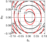
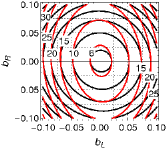
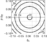
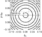
Figure 1: (color online) The total decay width contours of the tBESS vector triplet. The upper row displays the $V^{0}$ decay widths (numeric labels in GeV) in the $(b_{L},b_{R})$ plane for the cases of $p=1$ (black circlelike contours) and $p=0$ (red elliptic contours). The bottom row displays the $V^{\pm}$ decay widths (in GeV) in the $(b_{L},pb_{R})$ plane. The graphs in the left and right columns correspond to $g^{\prime\prime}=10$ and $g^{\prime\prime}=20$, respectively. All graphs have been plotted for $M_{V^{0}}=1$ TeV and $\lambda_{L}=\lambda_{R}=0$.

The $\lambda$ parameters were set to zero. As can be seen in Table 1, the dominant coupling terms depend solely on $b$ parameters, while the contributions of the $\lambda$-dependent terms are always suppressed by the nondiagonal elements of the mixing matrices $O^{N}$ and $O^{C}$. Hence, the effect of nonzero $\lambda$’s on the decay widths is negligible if the parameters assume the values dictated by the low-energy limits (for the limits, see Subsection III.3).

Note that the contours of the constant decay widths in the $b_{L}$-$b_{R}$ space form ellipses with the eccentricities depending on the value of the $p$ parameter. When $p=1$ the ellipses approach a circular shape. In the case of the charged resonance the total decay width is not a function of $b_{R}$ and $p$ separately. It rather depends on the product of the two parameters. Finally, the ellipses/circles do not have their centers, which indicate the points of the minimal widths, at the origin of the parametric space. The centers are shifted from the origin but the shift decreases with growing $g^{\prime\prime}$. The centers reach the origin when $g^{\prime\prime}\rightarrow\infty$.

Except for the special regions of the parametric space which will be discussed in Sec. III.4 the vector triplet predominantly decays to the electroweak gauge bosons, $W^{\pm}$ and $Z$, and/or to the third generation of quarks. Figures 2 and 3 depict the branching ratios of the neutral and charged resonances, respectively, for the gauge boson and top/bottom quark channels.

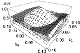
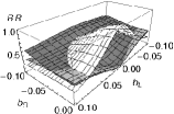
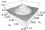
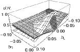
Figure 2: The branching ratio of $V^{0}$ to the $W^{+}W^{-}$ (white), $t\bar{t}$ (dark gray), and $b\bar{b}$ (light gray) decay channels in the $(b_{L},b_{R})$ plane for the cases of $p=0$ (upper row) and $p=1$ (bottom row). In all graphs $g^{\prime\prime}=20$, $M_{V^{0}}=1$ TeV, and $\lambda_{L}=\lambda_{R}=0$. The $b_{R}=0$ dissections of the graphs are shown in the right column.

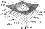
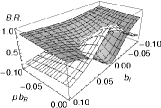
Figure 3: The branching ratio of $V^{\pm}$ to the $WZ$ (white) and $tb$ (gray) decay channels in the $(b_{L},pb_{R})$ plane. Other parameters: $g^{\prime\prime}=20$, $M_{V^{0}}=1$ TeV, and $\lambda_{L}=\lambda_{R}=0$. The $pb_{R}=0$ dissection of the left graph is shown on the right-hand side.

As expected, the quark decay channels prevail when the moduli of $b$ parameters assume sufficiently large values. Details depend on other parameters of the model, $g^{\prime\prime}$, $M_{V^{0}}$, and $p$. While the decay widths to the third generation of quarks grow with $g^{\prime\prime}$ — namely, they are proportional to $g^{\prime\prime 2}$ — the decay widths to $W^{\pm}$ and $Z$ are proportional to $1/g^{\prime\prime 2}$.

III.2 Tree-level unitarity constraints

The SM without the Higgs is not renormalizable and its amplitudes violate unitarity at some energy. In particular, when the longitudinal electroweak gauge-boson scattering is considered the partial wave tree-level unitarity is violated at $\sqrt{s}=1.7$ TeV DominiciNuovoCim . The result has been obtained using the Equivalence Theorem EquivalenceTheoremRenorm ; EquivalenceTheoremNonRenorm approximation of the $W_{L}^{+}W_{L}^{-}$, $Z_{L}Z_{L}$, $W_{L}^{\pm}Z_{L}$, and $W_{L}^{\pm}W_{L}^{\pm}$ scattering by the pionic scattering amplitudes of the $SU(2)_{L}\times SU(2)_{R}/SU(2)_{L+R}$ nonlinear sigma model. The matrix of the $a_{0}$ partial waves of all the scattering amplitudes was formed, where the zero index at $a_{0}$ indicates the $J=0$ angular momentum. The $S$-matrix unitarity implies that the maximum of the moduli of the $a_{0}$ matrix eigenvalues should be less than 1 LeeQuiggThacker77 . This condition leads to the energy restriction cited above.

To obtain the unitarity constraints for the tBESS model an analogical procedure has been applied. The only difference is that the $W_{L}^{+}W_{L}^{-}$, $Z_{L}Z_{L}$, $W_{L}^{\pm}Z_{L}$, and $W_{L}^{\pm}W_{L}^{\pm}$ scattering amplitudes can also proceed through the exchange of the new resonances. It modifies the amplitude expressions so that they read

$${\cal M}(W_{L}^{+}W_{L}^{-}\rightarrow W_{L}^{+}W_{L}^{-}) = A(s,t,u)+A(t,s,u),$$

$${\cal M}(Z_{L}Z_{L}\rightarrow Z_{L}Z_{L}) = 0,$$

$$\sqrt{2}{\cal M}(W_{L}^{+}W_{L}^{-}\rightarrow Z_{L}Z_{L}) = A(s,t,u),$$

$${\cal M}(W_{L}^{\pm}Z_{L}\rightarrow W_{L}^{\pm}Z_{L}) = A(t,s,u),$$

$$\sqrt{2}{\cal M}(W_{L}^{\pm}W_{L}^{\pm}\rightarrow W_{L}^{\pm}W_{L}^{\pm}) = A(t,s,u)+A(u,t,s),$$

$$A(s,t,u)=\frac{s}{4v^{2}}(4-3\alpha)+\frac{\alpha M_{V}^{2}}{4v^{2}}[f(t,u)+f(u,t)],$$ (51)

where

$$f(t,u)=\frac{u-s}{t-M_{V}^{2}+iM_{V}\Gamma_{V}}.$$ (52)

The eigenvalues of the $a_{0}$ matrix based on the electroweak gauge-boson scattering amplitudes are functions of $\sqrt{s}$, $g^{\prime\prime}$, and $M_{V}$, when the $\alpha$ parameter has been replaced by $M_{V}$ using the leading order of the mass relation (24), $M_{V}=\sqrt{\alpha}vg^{\prime\prime}/2$. No couplings to fermions are assumed, therefore

$$\Gamma_{V}=\frac{M_{V}g^{\prime\prime 2}}{768\pi}\alpha^{2}=\frac{M_{V}^{5}}{48\pi v^{4}}\frac{1}{g^{\prime\prime 2}}.$$ (53)

Then, constraining the maximal eigenvalue modulus by unity results in the unitarity constraints depicted in Fig. 4.

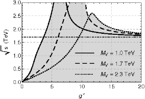
Figure 4: The tree-level unitarity constraints from the gauge-boson scattering obtained for various masses of the vector triplet: $M_{V}=1$ TeV (solid line), $1.7$ TeV (dashed), $2.3$ TeV (dotted). The horizontal dashed-dotted line is the Higgsless SM unitarity limit of 1.7 TeV. The shaded area indicates the region where the unitarity holds. No couplings to fermions are assumed.

If we require that the tBESS model amplitudes unitarity holds up to the same energy as for the Higgsless SM — $1.7$ TeV — the $g^{\prime\prime}$ parameter is restricted only from below. This bottom limit depends on $M_{V}$: $g^{\prime\prime}\stackrel{{\scriptstyle>}}{{\sim}}3,6$, and $9$, when $M_{V}=1.0,1.7$, and $2.3$ TeV, respectively. The tBESS model amplitudes can satisfy the unitarity also at higher energies, if $g^{\prime\prime}$ is properly restricted from above. One has to remember that nonrenormalizability of the model implies the upper limit on the applicability of the Equivalence Theorem EquivalenceTheoremNonRenorm . It holds for $E\leq 4\pi v\approx 3$ TeV. This sets the upper energy limit on any conclusions inferred from the use of the theorem.

It seems reasonable to demand that the unitarity constraint exceeds the mass of the $SU(2)_{HLC}$ resonance. If we require that the unitarity of the model holds up to the energy of $E=1.5M_{V}$ we obtain the unitarity allowed region in the $\Gamma_{V}$-$M_{V}$ plane shown in Fig. 5.

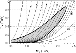
Figure 5: The allowed values (the shaded region) of the width and mass of the vector resonance assuming the unitarity saturation at or above $E=1.5M_{V}$. The lines crossing the plane indicate the points of the fixed values of $g^{\prime\prime}$. No couplings to fermions are assumed.

The lines of constant $g^{\prime\prime}$ values are superimposed over the unitarity allowed region. The graph suggests that the $M_{V}$ values which can be accommodated by the tBESS effective model cannot exceed $2.26$ TeV. If we wish to avoid wide resonances, we should stay at somewhat lower masses, say, up to about $1.5$ TeV. Recall that no decays to fermions have been involved when obtaining these conclusions.

The expression (51) is identical with that of the BESS model except for the decay width $\Gamma_{V}$ of the vector resonance. To reflect the impact of the fermion sector on the tBESS vector boson decay widths the third quark generation decay channels assuming no gauge-boson mixing and the massless quarks will be added. In this approximation, the neutral tBESS resonance decays to $W_{L}^{+}W_{L}^{-}+b\bar{b}+t\bar{t}$ and the charged one to $W_{L}^{\pm}Z_{L}+t\bar{b}/\bar{t}b$. Thus, the total decay width (53) will be modified as follows

$$\Gamma_{V}=\frac{M_{V}g^{\prime\prime 2}}{768\pi}\left[\alpha^{2}+12\beta^{2}(b_{L},b_{R},p)\right],$$ (54)

where $\beta=[b_{L}^{2}+b_{R}^{2}(1+p^{4})/2]^{1/2}$ for the neutral resonance and $\beta=[b_{L}^{2}+b_{R}^{2}p^{2}]^{1/2}$ for the charged one. In this approximation the decay width (54) is not a function of $\lambda$’s. As argued in Sec. III.1, dropping the $\lambda$ dependence has negligible consequences.

The vector resonance decay width makes the unitarity constraint sensitive to the parameters of the fermionic sector which are neatly packed into the $\beta$ parameter. The unitarity constraints based on the electroweak gauge-boson scattering amplitudes should be supplemented by the unitarity constraints derived from the scattering amplitudes with the participation of the top and bottom quarks. We have not performed the analysis in this paper. Thus, at this moment, we cannot tell whether and how the inclusion of the quark scattering processes influences the conclusions about the unitarity constraints. Nevertheless, the question of unitarity of top/bottom quark scattering amplitudes in similar situation to ours was treated in the literature Han1 ; Han2 . Their conclusions seem to suggest that the fermion amplitudes do not place stricter constraints than those based on the $ww\rightarrow ww$ scattering.

Considering the decay width (54) we have obtained the tBESS unitarity constraints which depend also on the $\beta$ parameter. There is an ambiguity which of the $\beta$ parameters should be used in the calculations of the unitarity limits. Both, neutral and charged, resonances contribute to the processes under consideration. This problem is a side effect of merging the contributions of two different Lagrangians, the nonlinear sigma model and the gauged tBESS model, into one decay width and as such it has no rigorous solution. It is the price to be paid for the shortcut we took in order to estimate the tBESS model behavior.

In our calculations, the neutral resonance $\beta$ parameter has been used. The $(g^{\prime\prime},\beta)$-dependent constraints for various values of $M_{V}$ can be seen in Fig. 6.

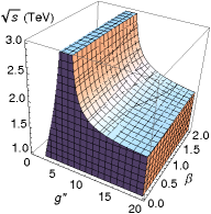
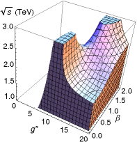
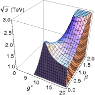
Figure 6: (color online) The tree-level unitarity constraints from the gauge-boson scattering obtained for various masses of the tBESS vector triplet. The decays to the third quark generation are included in evaluation of the vector resonance width; $\beta=[b_{L}^{2}+b_{R}^{2}(1+p^{4})/2]^{1/2}$. The graphs correspond to $M_{V}=1$ TeV, $2$ TeV, and $2.3$ TeV (from left to right).

It appears that for $M_{V}$ below $2$ TeV the $\beta$-dependence of the unitarity limit is negligible certainly when $\beta$ is below about $0.2$ and the limits of Fig. 4 remain valid. On the other hand, the higher the mass of the vector resonance, the stronger the effect of $\beta$. However, the higher values of $\beta$ are disfavored by the low-energy limits which will be discussed in Sec. III.3.

When we ask that the tBESS model unitarity is not violated below $1.5M_{V}$ we obtain the allowed regions in the $(\beta,g^{\prime\prime})$ plain. They are depicted in Fig. 7 for different values of $M_{V}$.

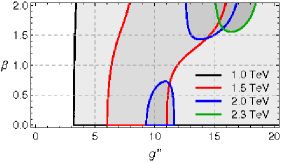
Figure 7: (color online) The allowed values (the shaded regions) of $\beta$ and $g^{\prime\prime}$ parameters assuming the unitarity saturation at or above $E=1.5M_{V}$ when the vector resonance width includes the decays to the third quark generation. The regions for different values of $M_{V}$ are depicted: $M_{V}=1$ TeV (black contour), $M_{V}=1.5$ TeV (red), $M_{V}=2$ TeV (blue), $M_{V}=2.3$ TeV (green). The gray color of the allowed regions darkens as the value of $M_{V}$ grows.

For $M_{V}=1$ TeV there is the rectangular quarter-plane, not bound from above, neither on the right-hand side, of the allowed values of the $\beta$ and $g^{\prime\prime}$ parameters. When the mass grows the allowed area shrinks and splits into discontinued regions. The upper bound on $g^{\prime\prime}$ appears once the required unitarity constraint crosses $1.7$ TeV which corresponds to the Higgsless SM unitarity limit plotted in Fig. 4. This occurs at $M_{V^{0}}=1.13$ TeV. Raising further the mass value results in the splitting of the allowed area into two separate regions. Even higher mass value causes the lower region to disappear. Of course, the critical mass values as well as all the constraints displayed in Fig. 7 are subject to the condition that the unitarity saturation takes place at least $50\%$ above the mass of the resonance. Changing the condition would alter the presented results.

When there were no fermion interactions, the unitarity saturation at $1.5M_{V}$, or higher, restricted the maximal vector resonance mass, for which the effective description works, to amount to $M_{V}=2.26$ TeV. On the other hand, Fig. 7 suggests that fermion interactions with $\beta\geq 1.6$ can bring masses higher than $2.26$ TeV back into the game. Because of the circumstances mentioned above this result should be supplemented by the analysis which would include the top/bottom scattering before reaching final conclusions on this matter.

III.3 Low-energy limits

The tBESS model is an effective description of a high-energy extension of the Higgsless SM. The existing electroweak precision data (EWPD) restrict tBESS induced deviations from the SM at the relevant energies. This experimental input results in the low-energy limits on the parameters of tBESS.

To obtain these limits we have to derive the low-energy Lagrangian by integrating out the vector triplet of the tBESS Lagrangian. It proceeds by taking the limit $M_{triplet}\rightarrow\infty$, while $g^{\prime\prime}$ is finite and fixed, and by substituting the equation of motion for the triplet fields obtained under these conditions.

The low-energy tBESS Lagrangian has been related to several independent measurements. First of all, to restrict $g^{\prime\prime}$ as well as the $b$ and $\lambda$ parameters, we have used the standard epsilon method for the EWPD EpsilonMethod1 ; EpsilonMethod2 . Another independent limit on $g^{\prime\prime}$ has resulted from the D0 measurement of $p\bar{p}\rightarrow WZX$ D0experimentTGV . Independently, the $b$ and $\lambda$ parameters have been restricted by the measurement of the $B\rightarrow X_{s}\gamma$ decay btosgData .

Let us briefly review the epsilon analysis. There are four epsilon parameters $\epsilon_{1},\epsilon_{2},\epsilon_{3},\epsilon_{b}$ which summarize the input of the SM weak physics at loop level and non-SM weak physics at tree and loop levels. The epsilons are extracted from data independently of $m_{t}$, $m_{H}$, and new physics parameters. Both $\epsilon_{1}$ and $\epsilon_{3}$ are obtained from the measurements of $A_{FB}^{\ell}$ and $\Gamma(Z\rightarrow\ell\ell)$. To obtain $\epsilon_{2}$ the measurement of $M_{W}/M_{Z}$ has to be supplemented. To obtain $\epsilon_{b}$ the measurement of $\Gamma(Z\rightarrow b\bar{b})$ has to be added. More details on deriving the low-energy limits from the epsilon analysis can be found in Appendix B.

The EWPD limit on $g^{\prime\prime}$ can be obtained from the $\epsilon_{3}$ parameter, using the relation

$$\epsilon_{3}=\left(\frac{g}{g^{\prime\prime}}\right)^{2}+\delta\epsilon_{3}^{SM},$$ (55)

where $\epsilon_{3}=0.005\,34\pm 0.000\,94$ is obtained from experiment EpsilonData , and the value of $\delta\epsilon_{3}^{SM}$ is the theoretical prediction which depends on $M_{H}$. Namely, $\delta\epsilon_{3}^{SM}=0.005\,89$, $0.006\,54$, and $0.006\,92$, for $M_{H}=0.3$, $1$, and $2$ TeV, respectively. Thus, the mean value of $\epsilon_{3}-\delta\epsilon_{3}^{SM}$ is negative and the Eq. (55) has no solution for $g^{\prime\prime}$. Nevertheless, the positive values of the difference are statistically admissible if we assume its normal distribution with the standard deviation taken from $\epsilon_{3}$. Then, the probability that the difference is positive amounts to $28\%$, $10\%$, and $5\%$, when $M_{H}=0.3$, $1$, and $2$ TeV, respectively. At the same time these numbers indicate the confidence level of $g^{\prime\prime}$ taking on any value. The likelihood that the $g^{\prime\prime}$ value lies anywhere below a given value $g_{0}^{\prime\prime}$ is depicted in Fig. 8.

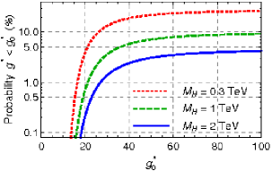
Figure 8: (color online) The probability that $g^{\prime\prime}$ lies anywhere below a given value of $g_{0}^{\prime\prime}$. It is based on $\epsilon_{3}$ parameter and depends on $M_{H}$ used for calculation of $\delta\epsilon_{3}^{SM}$. Plots for $M_{H}=0.3$ TeV (red dotted), $1$ TeV (green dashed), and $2$ TeV (blue solid) are shown.

While these numbers may seem low, there are some points to be made in order to see the situation in proper perspective. First of all, in the epsilon analysis, the approximation in which the tBESS loop-level contributions to $\epsilon$’s are replaced with the SM $M_{H}$-dependent loop-level contributions plus the net tBESS loop-level contributions is used. In addition, in the Eq. (55) the net tBESS loop terms, which are not necessarily negligible against $\delta\epsilon_{3}^{SM}$, have not been considered (see Table 6). Thus, it might be possible that using more precise formulae would significantly change the probability numbers shown above.

Secondly, in the original BESS model, $\epsilon_{3}$ depends, beside $g^{\prime\prime}$, also on the universal fermion parameter $b$. This dependency can compensate for the negativity of $\epsilon_{3}-\delta\epsilon_{3}^{SM}$. By turning off the direct coupling of the vector triplet to the light fermions, as we have done in the tBESS model, the dependency disappears and we face the tension between the negativity of $\epsilon_{3}-\delta\epsilon_{3}^{SM}$ and the positivity of $(g/g^{\prime\prime})^{2}$. Nevertheless, adding a new independent direct interaction of the light fermions with the vector triplet would be straightforward. It would be a natural extension of the tBESS model which is in line with the original motivation of the extraordinary role of the top quark. A new parameter, thus introduced to the Eq. (55), could compensate for the negativity of $\epsilon_{3}-\delta\epsilon_{3}^{SM}$ in the same way as the $b$ parameter in the BESS model does.

The gauge coupling $g^{\prime\prime}$ can also be restricted by the measurement of the gauge-boson self-interactions. In particular, the D0 measurement of $p\bar{p}\rightarrow WZX$ puts limits on the anomalous couplings of the effective $WWZ$ vertex D0experimentTGV . If the CP-invariant operators up to dimension four are considered, there are two free parameters, $g_{1}^{Z}$ and $\kappa_{Z}$, in the effective $WWZ$ vertex HagiwaraTGV . In the tBESS model, the two parameters coincide, $g_{1}^{Z}=\kappa_{Z}$, and depend on a single non-SM parameter, namely $g^{\prime\prime}$. Note that this is different from the BESS model where $g_{1}^{Z}$ (which, again, equals to $\kappa_{Z}$) depends also on the universal couplings of the vector triplet with fermions. The $D0$ measurements provide separate limits on $g_{1}^{Z}$ and $\kappa_{Z}$. Since $g_{1}^{Z}=\kappa_{Z}$ in the tBESS model, we consider the stronger of these limits to derive the restriction for $g^{\prime\prime}$. The obtained lower bound reads $g^{\prime\prime}\geq 3.4\;(95\%\mbox{C.L.})$.

The $b$ and $\lambda$ parameters are restricted by the measurement of $B\rightarrow X_{s}\gamma$ which puts limits on the anomalous $\kappa_{R,L}^{Wtb}$ parameters of the $W^{\pm}t_{R,L}b_{R,L}$ vertices btosgData ; LariosKappaAnalysis . In tBESS, these anomalous couplings are functions of the model’s parameters. It implies the low-energy limits on $b_{L}-2\lambda_{L}$ and $b_{R}+2\lambda_{R}$ for given values of $g^{\prime\prime}$ and $p$. The limits for various values of $p$ and $g^{\prime\prime}=10$ are shown in Fig. 9.

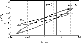
Figure 9: The $90\%$ C.L. $B\rightarrow X_{s}\gamma$ allowed regions of the $b$ and $\lambda$ parameters when $g^{\prime\prime}=10$. The allowed regions form closed elliptical bands; the darkest gray correspond to $p=0$, the lightest to $p=1$, with $p=0.5$ in between. When $p=0$, only parts of two parallel bands of an “infinite” ellipse can be seen.

The case of $g^{\prime\prime}\rightarrow\infty$ introduces a change not distinguishable in the graph.

Both $\epsilon_{1}$ and $\epsilon_{b}$ parameters can provide independent EWPD limits on the same combinations of $b$’s and $\lambda$’s as in the previous case. However, to the limits based on the $\epsilon_{b}$ parameter a qualification applies. The tBESS interactions are more general than the restriction imposed on the anomalous vector and axial-vector couplings of the bottom quark in the definition of $\epsilon_{b}$ EpsilonMethod2 . The definition assumes that these couplings are not independent of each other. Thus, $\epsilon_{b}$ can be used to derive the low-energy limits on the tBESS fermion parameters under this additional assumption only. In particular, the following condition must hold: either $p=0$, or $b_{R}=-2\lambda_{R}$. As far as the limits derived from $\epsilon_{1}$ are concerned, no such restrictions apply.

The intersections of the $\epsilon_{1}$ and $\epsilon_{b}$ based regions for $g^{\prime\prime}=10$ and $\infty$, and $p=0$ are depicted in Fig. 10. The cut-off scale $\Lambda$ of the low-energy effective theory is reasonable to be put equal to the mass of the vector resonance. In the figure, the graphs for $\Lambda=1$ TeV and $\Lambda=2$ TeV are displayed. The shaded areas of Fig. 10 lie completely inside the region allowed by the $B\rightarrow X_{s}\gamma$ decay. Thus, they can also be considered as the combined allowed region of the epsilon and $B\rightarrow X_{s}\gamma$ methods when $p=0$.

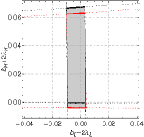
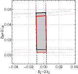
Figure 10: (color online) The intersecting parts of the $90\%$ C.L. allowed regions derived from $\epsilon_{1}$ (horizontal strip) and $\epsilon_{b}$ (vertical strip). The $\epsilon_{b}$ region assumes that $p=0$. The $\epsilon_{1}$ region is not sensitive to $p$. The black contours correspond to $g^{\prime\prime}=10$ and the red ones to $g^{\prime\prime}\rightarrow\infty$. The cut-off scales considered are $\Lambda=1$ TeV (left) and $\Lambda=2$ TeV (right).

If $b_{R}=-2\lambda_{R}$ and $p$ is arbitrary, the intersection of the $90\%$ C.L. regions of $\epsilon_{1}$, $\epsilon_{b}$, and $B\rightarrow X_{s}\gamma$, when $\Lambda=1$ TeV, reads

$$-0.009\leq\;b_{L}-2\lambda_{L}\;\leq 0.004.$$ (56)

This interval is virtually independent of $g^{\prime\prime}$. When $\Lambda=2$ TeV the regions have no common intersection at the given confidence level and for any value of $g^{\prime\prime}$.

If neither $p=0$, nor $b_{R}=-2\lambda_{R}$, the low-energy restrictions are provided by $\epsilon_{1}$ only as far as the epsilon parameters are considered. The restrictions are represented by the horizontal strips in Fig. 10.

In this case, the $\epsilon_{b}$-based restriction can be substituted for by the low-energy limit obtained directly from the measurement of the $\Gamma(Z\rightarrow b\bar{b})$ decay employing Eq. (11) of EpsilonMethod2 . Details of the calculation can be found in Appendix C.

In Fig. 11, the $90\%$ C.L. regions based on $\epsilon_{1}$, $\Gamma(Z\rightarrow b\bar{b})$, and $B\rightarrow X_{s}\gamma$, and their intersections are shown. Various combinations of the $p$, $g^{\prime\prime}$, and $\Lambda$ values are considered. It can be seen that for some combinations the intersections are restricted by the $B\rightarrow X_{s}\gamma$ measurement. In some cases some combinations are excluded completely; e.g. when $p=1,g^{\prime\prime}=10,\Lambda=2$ TeV.

In Fig. 11, for the sake of comparison, the intersections based on $\epsilon_{b}$ are also shown. Even though they are not identical with the $\Gamma(Z\rightarrow b\bar{b})$ based contours for $p=0$, they are reasonably close to each other.

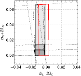
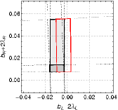
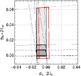
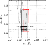
Figure 11: (color online) The intersections of the $\epsilon_{1}$ allowed regions (dotted lines) with the $\Gamma(Z\rightarrow b\bar{b})$ allowed regions (dashed lines) and the $B\rightarrow X_{s}\gamma$ allowed regions (dash-dotted lines). All regions are $90\%$ C.L. The $\Gamma(Z\rightarrow b\bar{b})$ regions are shown for $p=0$ (vertical strip), $p=0.5$ (middle tilted), and $p=1$ (the most tilted). The first row of the figures corresponds to $g^{\prime\prime}=10$, the second row to $g^{\prime\prime}=\infty$. The left column of figures corresponds to $\Lambda=1$ TeV, the right column to $\Lambda=2$ TeV. The shaded areas represent the intersections of all the regions for $p=0$ (the lightest gray), $p=0.5$ (middle gray), and $p=1$ (the darkest gray). The empty region with the red solid boundary corresponds to the $\epsilon_{b}$ based intersection taken from Fig. 10.

There are no low-energy limits on the values of the $b$ and $\lambda$ parameters individually. Thus, in principle, $b$’s and $\lambda$’s can be tuned to any values if their sum/difference falls within the allowed interval. However, if one does not wish to admit a fine-tuning of the parameters, it is in place to add some ad hoc restriction; say, the absolute values of the $b_{L,R}$ or $\lambda_{L,R}$ parameters should not be greater than 10 times the size of the allowed interval for $b_{L,R}\mp 2\lambda_{L,R}$. This way, the fine-tuning would not go below $10\%$. For example, if we apply this restriction to the limit for $p=0$, we obtain $|b_{L}|\leq 0.13$. Of course, at the same time the $\lambda$ parameters must fall in the strip $b_{L}-0.003\leq 2\lambda_{L}\leq b_{L}+0.010$.

In the BESS model, as well as in many other models of strong ESB and in the most common extra-dimensional Higgsless theories, the new vector resonances must be rather fermiophobic in order to satisfy the EWPD limits. There are ways how to remove this restriction found in the literature: e.g. the degenerated BESS model DBESS and the four-site Higgsless model 4siteExtraDimDBESS . The top-BESS model provides another alternative which does not suffer from this restriction.

The parameters $b_{L}$ and $b_{R}$ correspond to the BESS parameters $b$ and $b^{\prime}$ through the relations $b_{L}=b/(1+b)$ and $b_{R}=b^{\prime}/(1+b^{\prime})$. The authors of the BESS model BESS used $\epsilon_{3}$ to derive the low-energy limits for $b$ LowEBESS . We have updated the limits for the BESS model using the same epsilon values EpsilonData as for deriving the limits of the tBESS fermion parameters. When $g^{\prime\prime}=10$, we have obtained

$$0.008\leq b\leq 0.015\;\;\;(90\%\;\mbox{C.L.}).$$ (57)

Thus, the limit on $b_{L}$ obtained by the combination of the low-energy bounds and the no-fine-tuning requirement is significantly less restrictive, than the low-energy limit for $b$.

In the BESS model the universal right fermion coupling $b^{\prime}$ is usually set to zero due to the reasons mentioned before. In the tBESS model, the low-energy limits on $b_{R}$ can be even less restrictive than those on $b_{L}$ when $p$ approaches zero.

III.4 The Death Valley effect

The interplay of the direct and indirect couplings of the vector triplet with fermions can diminish or even zero a particular top/bottom quark channel decay width of the vector resonance for some nonzero values of the $b$ parameters. Thus, it might happen that even though the direct couplings of the vector resonance to the top and/or bottom quark are nontrivial the resonance will not decay through the given quark channel. Or, the particular decay will be suppressed below the value that would be implied by the indirect couplings alone.

Figure 12 shows the area of the $b_{L}$-$b_{R}$ parametric space where the decay width of $V^{0}\rightarrow t\bar{t}$ is equal to or lower than the corresponding value generated by the indirect couplings alone. We call this region the Death Valley (DV) because that is where the resonance decay through the particular decay channel deteriorates or even dies out.

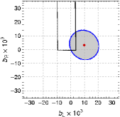
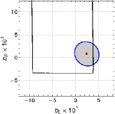
Figure 12: (color online) The Death Valley regions (shaded areas) of the $V^{0}\rightarrow t\bar{t}$ decay for $M_{V^{0}}=1$ TeV and $g^{\prime\prime}=10$ (left) and $g^{\prime\prime}=20$ (right). The red dot indicates values for which the corresponding partial decay width is equal to zero. The low-energy allowed region for $\lambda_{L}=\lambda_{R}=0$, $p=0$, and $\Lambda=1$ TeV (solid line) is superimposed on the graphs.

The dot in the middle of the area indicates the parameter values for which the partial decay width is equal to zero. The DV shrinks and the zero width point moves to the origin of the parametric space as $g^{\prime\prime}$ grows. The DV region for $t\bar{t}$ channel does not depend on $p$. Its dependence on $\lambda$’s can be neglected.

There are the EWPD contours superimposed over the DV graphs in the figure to show which part of the allowed parameter values overlaps with the DV. Recall that the low-energy limits apply to the combination of $b$’s and $\lambda$’s rather than to the parameters alone. The low-energy limits depicted in Fig. 12 correspond to $\lambda_{L}=\lambda_{R}=0$. By choosing nonzero values for $\lambda_{L,R}$ the low-energy contours get shifted around the parameter space. There are acceptable values of $\lambda$’s leading to both extrema — (a) no overlap, and (b) the maximal overlap — of the DV and the low-energy allowed regions.

The DV regions of the $V^{0}\rightarrow b\bar{b}$ decay for $M_{V^{0}}=1$ TeV are shown in Fig. 13.

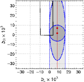
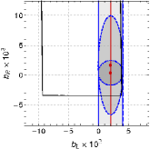
Figure 13: (color online) The Death Valley regions (shaded areas) of the $V^{0}\rightarrow b\bar{b}$ decay for $M_{V^{0}}=1$ TeV and $g^{\prime\prime}=10$ (left) and $g^{\prime\prime}=20$ (right). The dark gray area corresponds to the DV of $p=1$, the medium gray area to $p=0.5$, and the light gray region to $p=0$. The lower ($p=1$) and higher ($p=0.5$) red dots indicate the $(b_{L},b_{R})$ values for which the partial decay width is equal to zero. The middle red line corresponds to the $(b_{L},b_{R})$ values of the minimal $b\bar{b}$ decay width when $p=0$. The low-energy allowed region for $p=0$, $\lambda_{L}=\lambda_{R}=0$, and $\Lambda=1$ TeV is superimposed on the graphs.

In this case the DV region is of elliptical shape and depends on $p$. When $p=0$ the DV is an unbound strip in the $b_{R}$ direction. As $p$ decreases from 1 to 0 the $b_{R}$ coordinate of the zero width dot grows, reaching infinite value for $p=0$. Since $p=0$ turns off the $b_{R}$ coupling for any value of $b_{R}$, the indirect interaction of the vector triplet with the right bottom quark cannot be compensated by its direct analogue. Therefore, the $V^{0}\rightarrow b\bar{b}$ decay width cannot be equal to zero for any finite values of the $b$ parameters when $p=0$. Nevertheless, there will be the minimal value of the width at a fixed value of $b_{L}$ and any value of $b_{R}$.

Note that if $g^{\prime\prime}=10$ the DV area is equal or larger than the EWPD region. If we change the $\lambda_{L}$ value of the left-hand side graph of Fig. 13 to $\lambda_{L}=0.006$ the low-energy contours get shifted to the right and find themselves inside the DV’s. Thus, in this case the EWPD admit only $b_{L,R}$ values which lie inside the DV.

The DV’s for the quark decay of the charged resonance, $V^{\pm}\rightarrow t\bar{b}/\bar{t}b$, are shown in Fig. 14.

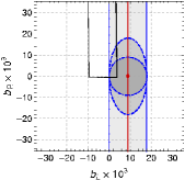
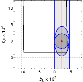
Figure 14: (color online) The Death Valley regions (shaded areas) of the $V^{\pm}\rightarrow t\bar{b}/\bar{t}b$ decay for $M_{V^{0}}=1$ TeV and $g^{\prime\prime}=10$ (left) and $g^{\prime\prime}=20$ (right). The dark gray area corresponds to the DV of $p=1$, the medium gray area to $p=0.5$, and the light gray region to $p=0$. The red dot ($p=1$ and $p=0.5$) and the red line ($p=0$) indicate the $(b_{L},b_{R})$ values for which the corresponding partial decay width is equal to zero. The low-energy allowed region for $p=0$, $\lambda_{L}=\lambda_{R}=0$, and $\Lambda=1$ TeV is superimposed on the graphs.

As in the case of the $b\bar{b}$ channel the DV depends on $p$. If $p=0$, its elliptical shape turns into the $b_{R}$-unbound strip. The position of the zero width point does not depend on $p$, if $p>0$. If $p=0$, the zero width point turns into a straight line of a fixed $b_{L}$ value and any $b_{R}$ value. As in the previous case, it is possible to hide the low-energy allowed regions inside the corresponding DV; $\lambda_{L}=0.006$ would make the job as it did in the case of $V^{0}\rightarrow b\bar{b}$.

III.5 Scattering processes

The main goal of the construction and study of the tBESS model is to provide an effective tool for the description and analysis of the possible experimental situation observed at the LHC and the ILC. Even though the analysis of sensitivity of particular scattering processes to the tBESS parameters is not within the scope of this paper we would like to discuss two features of the tBESS model which can prove important when such analysis will be performed.

Hiding the peak

The Death Valley effect can hide signals expected in scattering processes. There might be new physics materialized through the existence of the new vector resonances as well as nonzero values of the $b$ parameters, yet it does not have to reveal itself in an experiment. In particular, even if the tBESS resonances exist and couple to the third quark generation we do not have to see a peak in the scattering experiments for certain final states containing top and/or bottom quarks. This would occur if the model parameters happened to have their values inside the DV region. More precisely, the region, in which the resonance peak in a scattering process is lower than the peak due to the indirect couplings to fermions, can slightly differ from the DV region. It is due to the interference effects between signal and nonsignal amplitudes of the process. Nevertheless, we will not elaborate on this in this paper.

To illustrate the DV effect on the scattering amplitudes we have plotted the cross sections for five processes: $e^{-}e^{+}\rightarrow t\bar{t}/b\bar{b}/W^{+}W^{-}$ and $u\bar{d}\rightarrow t\bar{b}/W^{+}Z$. The cross sections are evaluated for $M_{V^{0}}=1$ TeV and $g^{\prime\prime}=20$ at four different parameter space points (PSP) which are specified in Table 2.

Table 2: Parameter space points (PSP) at which the cross sections in Fig. 15 were calculated.

PSP	$p$	$b_{L}$	$b_{R}$	$\lambda_{L}$	$\lambda_{R}$
1	0	0	0	0	0
2	0	-0.01	0.03	0	0
3	0	0.009	0.03	0.006	0
4	0	0.0098	0.0034	0.006	0

The points were chosen to demonstrate how the tBESS resonance peak behaves if PSP lies inside or outside the DV. Of course, the gauge-boson processes are sensitive to the choice of PSP only through the resonance decay width. The nonzero values of $\lambda_{L}$ have been chosen to shift the low-energy allowed region so that it includes the given PSP. The cross section at the peak region is not significantly affected by the $\lambda$-values, though.

The PSP=1 graph in Fig. 15 shows the cross sections of the five processes when there is no direct coupling of the vector resonance to fermions.

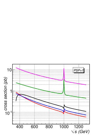
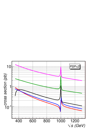
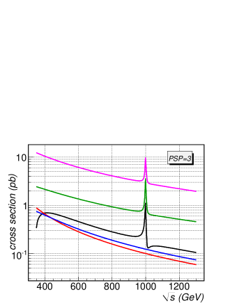
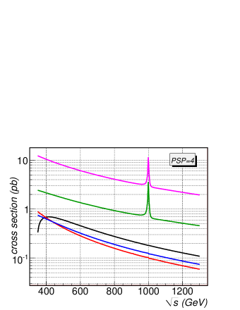
Figure 15: (color online) The cross sections of the $e^{-}e^{+}\rightarrow t\bar{t}/b\bar{b}/W^{+}W^{-}$ and $u\bar{d}\rightarrow t\bar{b}/W^{+}Z$ processes for $M_{V^{0}}=1$ TeV and $g^{\prime\prime}=20$. The four graphs correspond to the four parameter space points specified in Table 2. Each graph displays plots of all five processes. From top to bottom: $e^{-}e^{+}\rightarrow W^{+}W^{-}$ (magenta), $u\bar{d}\rightarrow W^{+}Z$ (green), $e^{-}e^{+}\rightarrow t\bar{t}$ (black), $u\bar{d}\rightarrow t\bar{b}$ (blue), $e^{-}e^{+}\rightarrow b\bar{b}$ (red).

While there are clear $1$ TeV resonance peaks in the gauge-boson channels the top/bottom channel processes exhibit only small peaks.

PSP=2 was chosen far away from the DV’s of all three top/bottom channels. Thus we expect to see large $1$ TeV peaks in all five cross sections. Indeed, the PSP=2 graph of Fig. 15 shows exactly that behavior.

PSP=3 lies at the bottoms of the DV’s for $b\bar{b}$ and $t\bar{b}$ channels. On the other hand, for the $t\bar{t}$ channel the PSP is far away from the channel’s DV. In accordance with that the PSP=3 graph in Fig. 15 shows the $1$ TeV resonance peak only in the $e^{-}e^{+}\rightarrow t\bar{t}$ cross section, other two top/bottom final state graphs being flat.

PSP=4 is localized at the bottom of the DV’s of all three top/bottom processes. Indeed, in their cross sections, no $1$ TeV peak can be found in the PSP=4 graph of Fig. 15.

Note that since $p=0$ for all PSP’s $b_{R}$-related couplings are effectively set to zero in the processes $e^{-}e^{+}\rightarrow b\bar{b}$ and $u\bar{d}\rightarrow t\bar{b}$.

Drell-Yan processes

The fundamental process for probing the mechanism of ESB is the electroweak gauge boson (EWGB) scattering, $WW\rightarrow WW$, where $W=W^{\pm},Z$. No matter what is the theory behind ESB, it must leave its footprints in all processes containing $WW\rightarrow WW$ as a part of their Feynman diagrams. That is why major attention in the literature has always been paid to the processes which realize the EWGB scattering through $WW$ fusion, either at the LHC or at the ILC VLVLtoVLVL (see also Ref. snowmass and references therein). Particularly, if there is a vector resonance associated to the ESB sector, one would expect that it strongly couples to the longitudinal components of the massive electroweak gauge bosons and we should detect its existence through these processes.

Beside the EWGB fusion processes, the processes with the associated production of a resonance $R$, $ee/qq\rightarrow RW$, where $R$ is radiated of the final EW gauge boson, and decays subsequently into the pair of EW gauge bosons, $R\rightarrow WW$, can also probe the ESB sector.

The answer to the question how the ESB vector resonance couples to the SM fermions is very much model-dependent. There are many strong ESB models where the EWPD, namely the limits on the $\epsilon_{3}$ parameter, suppress the direct interactions of the new vector resonances with fermions. For example, the BESS model vector triplet is fermiophobic. Also, the most common Higgsless extra-dimensional theories, including the three-site one 3siteExtraDimBESS , are fermiophobic 4siteExtraDimDBESS . If this is the case, the experimental search for the vector resonance is bound to the fusion and associated production processes mentioned above.

In the case of nonfermiophobic models, like the degenerated BESS model DBESS and the four-site Higgsless extra-dimensional model 4siteExtraDimDBESS , the stronger direct couplings to fermions bring up new candidate processes for testing the ESB vector resonances. To discover the new resonances and test their relationship to fermions the scope of candidate processes can be widened to the EWGB fusion and the associated resonance production where the EW gauge bosons at one or both ends of resonance propagators are replaced with fermions. This also includes the Drell-Yan processes at the LHC, as well as the s-channel resonance production at the ILC. Indeed, these processes were studied in the literature DominiciNuovoCim ; 4siteExtraDimDBESS and found promising.

Processes where the new resonance interacts with top quarks in particular do not only provide supplemental opportunities to discover the new vector resonances, they can also probe the relationship between ESB physics and physics of the top quark Lee ; snowmass . Many papers focus on processes with $ww\rightarrow t\bar{t}$ scattering involved VLVLtoTT .

Because of the nonuniversality of its interactions with the SM fermions the tBESS vector triplet does not fit to either of the two categories mentioned above. The tBESS model admits strong direct couplings to top and bottom quarks and none to the light SM fermions. Of course, there are the mixing-induced indirect couplings to the light fermions which are suppressed. Thus, when searching for candidate processes to probe the tBESS model one would tend to avoid those where the vector triplet couples to light fermions. However, the existing studies of the vector resonances with nonuniversal couplings to fermions Han1 ; Han2 ; Han3 show that these naive expectations are not always correct. At the LHC, the $WW\rightarrow tt$ fusion process is overwhelmed by the QCD background. On the other hand, the Drell-Yan processes and the resonance associated production with top/bottom quark final states appear detectable. The Drell-Yan processes can compete because the suppressed interactions of the resonance with light quarks can be compensated for by their higher luminosities in proton-proton collisions.

Our preliminary study STM2008 ; InProgress of sensitivity of the LHC Drell-Yan processes to the tBESS resonances at $M_{V^{0}}=1$ TeV suggests that while $pp\rightarrow t\bar{t}X/b\bar{b}X$ is overwhelmed by the gluon-gluon background and thus insensitive to the tBESS resonance, the $pp\rightarrow t\bar{b}X/W^{+}W^{-}X/W^{\pm}ZX$ processes yield quite promising signals.

In this paper we do not aim to perform systematic study of the tBESS model testing at either of the existing or future colliders. Nevertheless, as an illustration, in Fig. 16 we show the invariant mass distributions for the final state particles of the $pp\rightarrow t\bar{b}X/W^{+}W^{-}X/W^{\pm}ZX$ processes at the LHC.

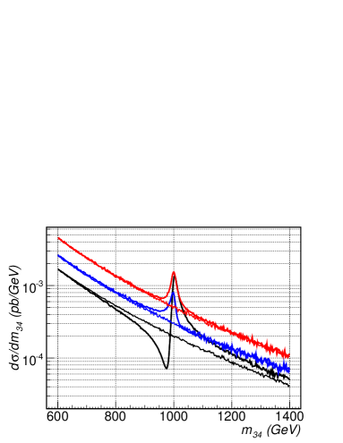
Figure 16: (color online) The invariant mass distributions for the final state particles of the $pp\rightarrow W^{+}W^{-}X$ (top red line), $pp\rightarrow(W^{+}Z+W^{-}Z)X$ (middle blue line), and $pp\rightarrow(t\bar{b}+b\bar{t})X$ (bottom black line) processes at the LHC for $\sqrt{s}=14$ TeV and $M_{V^{0}}=1$ TeV, $g^{\prime\prime}=20$, $p=0.5$, $b_{L}=-0.072$, $b_{R}=0.074$, $\lambda_{L}=\lambda_{R}=-0.03$. The thinner lines depict the SM predictions assuming $M_{Higgs}=115$ GeV.

The collision energy is $\sqrt{s}=14$ TeV and $M_{V^{0}}=1$ TeV. Other tBESS parameters read $g^{\prime\prime}=20$, $p=0.5$, $b_{L}=-0.072$, $b_{R}=0.074$. If $\lambda_{L}=\lambda_{R}=-0.03$ this PSP finds itself in the low-energy allowed region of the tBESS parametric space, away from the DV’s of all decay channels. The mass of the charged resonance is $M_{V^{\pm}}=999.84$ GeV. The only cuts applied to all processes exclude the forward and backward scattering angles for which their cosines are either below $-0.99$ or above $0.99$. The Cabibbo-Kobayashi-Maskawa matrix mixing is ignored in the calculations. The total cross sections obtained under these conditions read

$$\sigma(t\bar{b}+b\bar{t}) = \phantom{3}4.18\;(\phantom{3}4.09)\;\;\mbox{pb},$$

$$\sigma(W^{+}Z+W^{-}Z) = 10.75\;(10.52)\;\;\mbox{pb},$$

$$\sigma(W^{+}W^{-}) = 31.85\;(31.29)\;\;\mbox{pb}.$$

The values in the round brackets correspond to the SM with $M_{Higgs}=115$ GeV. The cross sections of individual subprocesses are shown in Table 3.

Table 3: The tree-level cross sections of individual subprocesses contributing to the processes calculated in Fig. 16. $M_{Higgs}=115$ GeV is assumed for the SM.

$pp\rightarrow t\bar{b}X/b\bar{t}X$
$\sigma$ (pb)	$u\bar{d}$	$c\bar{s}$	$d\bar{u}$	$s\bar{c}$
tBESS	1.05	0.16	0.73	0.16
SM	1.02	0.15	0.72	0.15
$pp\rightarrow W^{+}ZX/W^{-}ZX$
$\sigma$ (pb)	$u\bar{d}$	$c\bar{s}$	$d\bar{u}$	$s\bar{c}$
tBESS	2.63	0.45	1.84	0.45
SM	2.57	0.44	1.80	0.44
$pp\rightarrow W^{+}W^{-}X$
$\sigma$ (pb)	$u\bar{u}$	$d\bar{d}$	$s\bar{s}$	$c\bar{c}$	$b\bar{b}$
tBESS	7.00	5.62	1.85	1.08	0.38
SM	6.88	5.52	1.81	1.06	0.37

The CTEQ6L1 parton distribution functions were used to obtain these results.

The vector resonance decay widths for the PSP at which the $pp$ processes were calculated are shown in Table 4.

Table 4: The partial decay widths of the vector resonance triplet at $M_{V^{0}}=1$ TeV, $g^{\prime\prime}=20$, $p=0.5$, $b_{L}=-0.072$, $b_{R}=0.074$, $\lambda_{L}=\lambda_{R}=-0.03$.

$V^{0}\rightarrow$	$W^{+}W^{-}$	$t\bar{t}$	$b\bar{b}$	$u\bar{u}$	$d\bar{d}$	total
width (GeV)	5.29	8.98	5.79	0.007	0.004	20.09
$V^{+}\rightarrow$	$W^{+}Z$	$t\bar{b}$		$u\bar{d}$		total
width (GeV)	5.40	13.10		0.010		18.53

Let us note that the $pp\rightarrow(t\bar{b}+b\bar{t})X$ process is sensitive to the direct fermion couplings through the $V^{\pm}tb$ vertex, the $pp\rightarrow(W^{+}Z+W^{-}Z)X$ process is only sensitive to $g^{\prime\prime}$ through the triple gauge vertex of $V^{\pm}W^{\pm}Z$, and the $pp\rightarrow W^{+}W^{-}X$ process is sensitive to the fermion couplings through the $V^{0}bb$ vertex and to $g^{\prime\prime}$ through the triple gauge vertex of $V^{0}W^{+}W^{-}$. In the $pp\rightarrow W^{+}W^{-}X$ case the sensitivity to fermion couplings is only through the $b\bar{b}\rightarrow W^{+}W^{-}$ component which contributes just a small fraction of the cross section. Nevertheless, this subprocess contributes significantly to the resonance peak.

In the ILC s-channel production the resonance must be produced through the annihilation of the light fermions which is a disadvantage for this kind of process. Nevertheless, Fig. 15 suggests that it might be worthwhile to study sensitivity of the ILC $e^{-}e^{+}\rightarrow V^{0}\rightarrow 2$ processes with the electroweak gauge bosons or top/bottom quarks in the final states. Our preliminary work InProgress ; 18KSF on this issue further supports this hope.

All cross section calculations in this section were performed at the tree-level using the CompHEP software CompHEP . For that sake, we have implemented the tBESS Lagrangian into the COMPHEP as one of its models.

IV Conclusions

The effective Lagrangian, the so-called top-BESS model, of an alternative scenario of ESB has been formulated and investigated. It is the effective description of beyond the SM hypotheses where new strong interactions are responsible for ESB. The tBESS model singles out the direct coupling of the vector triplet to the third quark generation only. Therefore, it is a suitable effective Lagrangian for theories where the top (and perhaps also bottom) quark play an outstanding role in new physics beyond the SM.

There is no direct coupling of the tBESS vector triplet to the light SM fermions. Thus, the vector triplet can couple to the light fermions only through indirect interactions induced by the mixing of the vector triplet with the electroweak gauge bosons.

The study of the electroweak gauge-boson scattering implies that the no-Higgs SM unitarity restriction of 1.7 TeV can be somewhat raised by the introduction of the tBESS vector triplet for the limited choice of the tBESS free parameters only. For example, when $M_{V^{0}}=1$ TeV, the tBESS unitarity up to $1.7$ TeV, at least, is guaranteed for $g^{\prime\prime}\stackrel{{\scriptstyle>}}{{\sim}}3$ and for any values of the fermion sector parameters $b_{L}$, $b_{R}$, $\lambda_{L}$, $\lambda_{R}$ and $p$. The unitarity allowed parameter region quickly shrinks if we require the unitarity limit higher then $2$ TeV. It seems that the strong couplings of the vector triplet with fermions might influence these conclusions. However, the analysis of the top/bottom quark scattering amplitudes would be required to settle this question. In addition, large values of the $b$ and $\lambda$ parameters are admissible only in the fine-tuning regime.

Confrontation of the tBESS model with the EWPD results in the low-energy limits on the model’s parameters. The $\epsilon_{3}$ parameter can accommodate any value of $g^{\prime\prime}$ with only quite low probability, e.g. $10\%$ when $M_{H}$ is set to 1 TeV in approximating the loop contributions to $\epsilon_{3}$. Nevertheless, there are good reasons not to take these numbers too seriously. For example, they can be altered by adding a new direct interaction of the vector triplet with light fermions to the tBESS model. There is also an independent lower limit on $g^{\prime\prime}$ set by the D0 measurements of the $WWZ$, $g^{\prime\prime}\geq 3.4$ ($95\%$ C.L.), which plays no significant role under the given circumstances.

The epsilon analysis combined with the $B\rightarrow X_{s}\gamma$ measurement restricts the expressions $b_{L}-2\lambda_{L}$ and $b_{R}+2\lambda_{R}$. The situation is complicated by the fact that due to its definition $\epsilon_{b}$ can be used to extract low-energy limits only if $p=0$ or $b_{R}=-2\lambda_{R}$. To obtain the restrictions for more general case of the tBESS model, we have used the measurements of the branching ratio for $Z\rightarrow b\bar{b}$ and the total decay width of the $Z$ boson. There are no low-energy limits on the individual $b$ and $\lambda$ parameters. However, if the fine-tuning of the $b$ and $\lambda$ parameters should not go below $10\%$ then $b_{L}$ and $\lambda_{L}$ might be as large as about $\pm 0.1$. Analogically, $b_{R}$ and $\lambda_{R}$ can be as large as about $\pm 0.7$ when $p=0$ or about $\pm 0.08$ when $p=1$. These numbers are $\Lambda$ dependent and, to a lesser extent, $g^{\prime\prime}$ dependent, though.

If the values of the $b_{L}$ and $b_{R}$ parameters lie in the Death Valley region, the top/bottom partial decay widths of the vector resonances diminish below the no-direct-coupling value. It is a consequence of the interplay of the direct and indirect fermion couplings of the vector triplet. If this occurred the resonance peak in a process where $V$ decays to top and/or bottom quarks could disappear even though the resonance exists and couples directly to the third quark generation.

Our calculations suggest that there are acceptable values of the tBESS parameters which can result in detectable signals at the LHC and/or the ILC. In particular, despite what would be the one’s first guess, it seems to be worthwhile to study the LHC Drell-Yan processes and the ILC $e^{+}e^{-}\rightarrow R$ processes with top/bottom quarks and EW gauge bosons in their final states in order to probe the top-BESS model. However, this is far from conclusive. It would need to perform a more systematic study focused on the process analysis. The next step in this direction might include more systematic scan of the parametric space, more realistic final states and cuts, and the inclusion of the backgrounds, at least.

Appendix A Transformation relations

The transformation relations of the basic mathematical objects used to build the tBESS effective Lagrangian are summarized in Table 5. Recall that the weak hypercharge $Y=T_{R}^{3}+(B-L)/2$, where $T_{R}^{3}$ is the third $SU(2)_{R}$ generator. Thus when $B-L=0$ then $Y=T_{R}^{3}\equiv Y_{R}$.

Table 5: The transformation relations of the basic mathematical objects used to build the tBESS effective Lagrangian.

Object	Global	Local
$\mbox{\boldmath$W$}_{\mu}=igW_{\mu}^{a}\tau^{a}$	$g_{L}\mbox{\boldmath$W$}_{\mu}g_{L}^{\dagger}$	$g_{L}\mbox{\boldmath$W$}_{\mu}g_{L}^{\dagger}+g_{L}\partial_{\mu}g_{L}^{\dagger}$
$\mbox{\boldmath$B$}_{\mu}=ig^{\prime}B_{\mu}Y$	$g_{R}\mbox{\boldmath$B$}_{\mu}g_{R}^{\dagger}$	$\mbox{\boldmath$B$}_{\mu}+g_{Y}\partial_{\mu}g_{Y}^{\dagger}$
$\mbox{\boldmath$V$}_{\mu}=ig^{\prime\prime}V_{\mu}^{a}\tau^{a}/2$	$h^{\dagger}\mbox{\boldmath$V$}_{\mu}h$	$h^{\dagger}\mbox{\boldmath$V$}_{\mu}h+h^{\dagger}\partial_{\mu}h$
$\xi_{L}$	$g_{L}\;\xi_{L}\;h$	$g_{L}(x)\;\xi_{L}\;h(x)$
$\xi_{R}$	$g_{R}\;\xi_{R}\;h$	$g_{Y_{R}}(x)\;\xi_{R}\;h(x)$
$U=\xi_{L}\xi_{R}^{\dagger}$	$g_{L}\;U\;g_{R}^{\dagger}$	$g_{L}(x)\;U\;g_{Y_{R}}^{\dagger}(x)$
$\bar{\omega}_{\mu}^{\parallel,\perp}$	$h^{\dagger}\;\bar{\omega}_{\mu}^{\parallel,\perp}\;h$	$h^{\dagger}(x)\;\bar{\omega}_{\mu}^{\parallel,\perp}\;h(x)$
$\psi_{L}$	$g_{BL}\;g_{L}\;\psi_{L}$	$g_{Y}(x)\;g_{L}(x)\;\psi_{L}$
$\psi_{R}$	$g_{BL}\;g_{R}\;\psi_{R}$	$g_{Y}(x)\;\psi_{R}$
$\chi_{L}=\xi_{L}^{\dagger}\psi_{L}$	$g_{BL}\;h^{\dagger}\;\chi_{L}$	$g_{Y}(x)\;h^{\dagger}(x)\;\chi_{L}$
$\chi_{R}=\xi_{R}^{\dagger}\psi_{R}$	$g_{BL}\;h^{\dagger}\;\chi_{R}$	$g_{BL}(x)\;h^{\dagger}(x)\;\chi_{R}$

Appendix B Low-energy limits from the epsilon analysis

In deriving the low-energy limits from the epsilon analysis we follow the approach of LowEBESS .

The fermion Lagrangian describing the anomalous interactions of the electroweak gauge bosons with the top and bottom quarks reads

$$\!\!\!\!\!\!\!{\cal L}_{(t,b)}^{anom} = \phantom{-}{\cal L}_{(t,b)}^{SM}-\sum_{h=L,R}\left\{\frac{e}{\sqrt{2}s_{\theta}}\kappa_{h}^{Wtb}(\bar{t}_{h}\!\not{\!\!W}^{+}b_{h}+\mbox{h.c.})\right.$$ (58)

$$\left.+\frac{e}{2s_{\theta}c_{\theta}}\left[\kappa_{h}^{Ztt}(\bar{t}_{h}\!\not{\!\!Z}t_{h})+\kappa_{h}^{Zbb}(\bar{b}_{h}\!\not{\!\!Z}b_{h})\right]\right\},$$

where $\kappa$‘s parameterize the deviations from the SM

$${\cal L}_{(t,b)}^{SM} = -\frac{2}{3}e\;\bar{t}\!\not{\!\!A}t+\frac{1}{3}e\;\bar{b}\!\not{\!\!A}b-\frac{e}{\sqrt{2}s_{\theta}}(\bar{t}_{L}\!\not{\!\!W}^{+}b_{L}+\mbox{h.c.})$$

$$-\frac{e}{2s_{\theta}c_{\theta}}\left[\left(1-\frac{4}{3}s_{\theta}^{2}\right)(\bar{t}_{L}\!\not{\!\!Z}t_{L})-\frac{4}{3}s_{\theta}^{2}({\bar{t}}_{R}\!\not{\!\!Z}t_{R})\right]$$

$$+\frac{e}{2s_{\theta}c_{\theta}}\left[\left(1-\frac{2}{3}s_{\theta}^{2}\right)(\bar{b}_{L}\!\not{\!\!Z}b_{L})-\frac{2}{3}s_{\theta}^{2}(\bar{b}_{R}\!\not{\!\!Z}b_{R})\right],$$

where electric charge $e$ and sinus theta $s_{\theta}$ are defined as

$$e=\sqrt{4\pi\alpha(M_{Z})},$$ (59)

$$s_{\theta}^{2}c_{\theta}^{2}=\frac{\sqrt{2}e^{2}}{8G_{F}M_{Z}^{2}}.$$ (60)

In the case of the tBESS model the $\kappa$ parameters read

$$\kappa_{L}^{Wtb} = -\left(\frac{b_{L}}{2}-\lambda_{L}\right)\left(1-h\right)-h,$$

$$\kappa_{R}^{Wtb} = p\left(\frac{b_{R}}{2}+\lambda_{R}\right)\left(1-h\right),$$

$$\kappa_{L}^{Ztt} = -\left(\frac{b_{L}}{2}-\lambda_{L}\right)-\frac{4}{3}h,$$

$$\kappa_{R}^{Ztt} = \left(\frac{b_{R}}{2}+\lambda_{R}\right)-\frac{4}{3}h,$$

$$\kappa_{L}^{Zbb} = \left(\frac{b_{L}}{2}-\lambda_{L}\right)+\frac{2}{3}h,$$

$$\kappa_{R}^{Zbb} = -p^{2}\left(\frac{b_{R}}{2}+\lambda_{R}\right)+\frac{2}{3}h,$$ (61)

and

$$h=\frac{s_{\theta}^{2}}{c_{2\theta}}\left(\frac{g}{g^{\prime\prime}}\right)^{2},$$ (62)

where $c_{2\theta}=c_{\theta}^{2}-s_{\theta}^{2}$.

The Lagrangian (58) can be confronted with the model independent epsilon analysis of the electroweak precision data EpsilonMethod1 ; EpsilonMethod2 . The new physics tree-level contributions to the epsilon parameters are functions of the $\kappa$‘s. Beside that, there are loop-level contributions $\delta\epsilon^{loops}$. Thus,

$$\epsilon=\epsilon^{tree}+\delta\epsilon^{loops},$$ (63)

where the loop contributions are of two kinds: the SM ones 4siteBESS and the new physics ones, $\delta\epsilon^{loops}\approx\delta\epsilon^{SM}+\delta\epsilon^{NP}$. We derive limits from the values of three epsilons — $\epsilon_{1},\epsilon_{3}$, and $\epsilon_{b}$ — including some radiative corrections as indicated in Table 6.

Table 6: The contributions to the individual epsilons. The included contributions are denoted by the checkmark (✓ ), the left-out (not calculated) contributions are denoted by the cross mark ($\times$).

	Tree	SM loops	NP loops
			$Wtb$	$Ztt$	$Zbb$
$\epsilon_{1}$	✓	✓	✓	✓	$\bm{\times}$
$\epsilon_{3}$	✓	✓	$\bm{\times}$	$\bm{\times}$	$\bm{\times}$
$\epsilon_{b}$	✓	✓	✓	✓	$\bm{\times}$

The restriction on $g^{\prime\prime}$ can be obtained from $\epsilon_{3}$. In the case of tBESS

$$\epsilon_{3}=\left(\frac{g}{g^{\prime\prime}}\right)^{2}+\delta\epsilon_{3}^{SM},$$ (64)

where the radiative correction beyond the SM have not been included. When $\delta\epsilon_{3}^{SM}$ is calculated, $M_{H}\sim$ TeV should be considered in order to imitate a strong ESB physics. In our calculations, we consider $M_{H}=1$ TeV, $2$ TeV, as well as $300$ GeV, for the sake of comparison. All these values result in $\delta\epsilon_{3}^{SM}$ larger than the experimental $\epsilon_{3}$. The consequences are discussed in Sec. III.3.

An expression, analogical to (64), was obtained for BESS in LowEBESS . In BESS though, $\epsilon_{3}$ is also a function of parameter $b$ which parameterizes the direct universal coupling of the vector triplet to the left fermions

$$\epsilon_{3}=-\frac{b}{2}+\left(\frac{g}{g^{\prime\prime}}\right)^{2}+\delta\epsilon_{3}^{SM}.$$

Thus, due to the universality, the limit for $g^{\prime\prime}$ depends on $b$ and vice versa (see Fig. 1 in LowEBESS ). When we change $g^{\prime\prime}$ from $10$ to $\infty$ the interval of the allowed $b$ values shifts by about $146\%$ of its length. In contrast, the tBESS allowed interval for $b_{L}-2\lambda_{L}$, when $b_{R}+2\lambda_{R}=0$, will shift by about $1\%$ only (see Fig. 10). Here, the sensitivity to $g^{\prime\prime}$ enters only through the $h$, as can be seen in (62).

Each of the parameters $\epsilon_{1}$ and $\epsilon_{b}$ restricts the combinations $b_{L}-2\lambda_{L}$ and $b_{R}+2\lambda_{R}$. The $\epsilon_{1}$ has no tree contribution, so we have

$$\epsilon_{1}=\delta\epsilon_{1}^{SM}+\delta\epsilon_{1}^{NP}.$$ (65)

On the other hand,

$$\epsilon_{b}=\epsilon_{b}^{tree}+\delta\epsilon_{b}^{SM}+\delta\epsilon_{b}^{NP},$$ (66)

where

$$\epsilon_{b}^{tree}=-\kappa_{L}^{Zbb}+\kappa_{R}^{Zbb}.$$ (67)

For the NP loop contributions to the $\epsilon_{1}$ and $\epsilon_{b}$ the relations from LariosKappaAnalysis have been adopted to obtain

$$\delta\epsilon_{1}^{NP} = \frac{3m_{t}^{2}G_{F}}{2\sqrt{2}\pi^{2}}\ln\frac{\Lambda^{2}}{m_{t}^{2}}\left[\kappa_{L}^{Wtb}\left(1+{\kappa_{L}^{Wtb}}\right)\right.$$ (68)

$$+\left.\left(\kappa_{R}^{Ztt}-\kappa_{L}^{Ztt}\right)\left(1-\kappa_{R}^{Ztt}+\kappa_{L}^{Ztt}\right)\right],$$

$$\delta\epsilon_{b}^{NP} = \frac{m_{t}^{2}G_{F}}{2\sqrt{2}\pi^{2}}\ln\frac{\Lambda^{2}}{m_{t}^{2}}$$ (69)

$$\times\left[\left(\kappa_{L}^{Ztt}-\frac{1}{4}\kappa_{R}^{Ztt}\right)\left(1+2\kappa_{L}^{Wtb}\right)\right],$$

where $\Lambda$ is the cut-off of the low-energy top-BESS model and it is set to 1 and 2 TeV. When calculating the SM radiative corrections we set $\Lambda=M_{H}$. The loop contributions coming from the anomalous $Zb\bar{b}$ vertex are not considered here. The mass of the top quark considered in the calculations is $m_{t}=172.7$ GeV.

The allowed values of the expressions $b_{L}-2\lambda_{L}$ and $b_{R}+2\lambda_{R}$ are given by the intersections of the $\epsilon_{1}$ and $\epsilon_{b}$ restrictions. However, recall that the $\epsilon_{b}$ restrictions can be applied only if $p=0$ or $b_{R}=-2\lambda_{R}$.

If $p=0$, the intersections form four disconnected regions. The intersection, which contains the origin, is depicted in Fig. 10. Two other intersections are ruled out by the $B\rightarrow X_{s}\gamma$ measurement. The fourth intersection and its dependence on $g^{\prime\prime}$ and $\Lambda$ is depicted in Fig. 17.

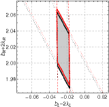
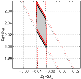
Figure 17: (color online) One of the four intersections of the $90\%$ C.L. $\epsilon_{1}$-allowed region (tilted strip) with the $90\%$ C.L. $\epsilon_{b}$-allowed region (vertical strip). Here, $p=0$ is assumed. Other two intersections are excluded by the $B\rightarrow X_{s}\gamma$ measurement and the fourth intersection is depicted in Fig. 10. The black contours correspond to $g^{\prime\prime}=10$ and the red ones to $g^{\prime\prime}\rightarrow\infty$. The cut-off scales considered are $\Lambda=1$ TeV (left) and $\Lambda=2$ TeV (right).

All the shown intersections of Fig. 17 lie completely inside the $B\rightarrow X_{s}\gamma$ allowed area. Despite that, we have not considered the fourth intersection values for the tBESS parameters in our analysis. The main reason is that the allowed interval of $b_{R}+2\lambda_{R}$ is too narrow. Using the values of $b_{R}$ and $\lambda_{R}$ of this region would correspond to fine-tuning below $10\%$, at least.

Appendix C Low-energy limits from the $\Gamma(Z\rightarrow b\bar{b})$ decay

To derive the low-energy limits from partial decay width $\Gamma(Z\rightarrow b\bar{b})$ the Eq. (11) of EpsilonMethod2 has been used

$$\Gamma_{b} = \frac{G_{F}{M_{Z}}^{3}}{6\pi\sqrt{2}}\beta\left(\frac{3-\beta^{2}}{2}{g_{bV}}^{2}+\beta^{2}{g_{bA}}^{2}\right)$$ (70)

$$\times N_{C}R_{QCD}\left(1+\frac{\alpha_{e}}{12\pi}\right),$$

where $\beta=\sqrt{1-4m_{b}^{2}/M_{Z}^{2}}$, $R_{QCD}=1+1.2a-1.1a^{2}-13a^{3}$ is the QCD correction factor, $a=\alpha_{s}(M_{Z})/\pi$, and $g_{bV}$ and $g_{bA}$ are vector and axial-vector couplings of the $b$ quark. We approximate the couplings by

$$g_{bV} = g_{bV}^{tBESS,tree}+\delta g_{bV}^{SM,loop},$$ (71)

$$g_{bA} = g_{bA}^{tBESS,tree}+\delta g_{bA}^{SM,loop},$$ (72)

where the first terms are the top-BESS tree-level couplings

$$g_{bV}^{tBESS,tree} = \left(1-4/3\;s_{\theta}^{2}-\kappa_{L}^{Zbb}-\kappa_{R}^{Zbb}\right)/2,$$ (73)

$$g_{bA}^{tBESS,tree} = \left(1-\kappa_{L}^{Zbb}+\kappa_{R}^{Zbb}\right)/2,$$ (74)

and the second terms are the SM loop contributions which can be expressed in terms of the epsilon analysis

$$\delta g_{bV}^{SM,loop} = \frac{1}{2}\left(1+\frac{\epsilon_{1}^{SM}}{2}\right)\left(1-\frac{4}{3}(1+\Delta k)s_{\theta}^{2}+\epsilon_{b}^{SM}\right)$$ (75)

$$-g_{bV}^{SM,tree},$$

$$\delta g_{bA}^{SM,loop} = \frac{1}{2}\left(1+\frac{\epsilon_{1}^{SM}}{2}\right)(1+\epsilon_{b}^{SM})-g_{bA}^{SM,tree},$$ (76)

where $g_{bV}^{SM,tree}=(1-4/3\;s_{\theta}^{2})/2$, $g_{bA}^{SM,tree}=1/2$, and

$$\Delta k=\frac{\epsilon_{3}^{SM}-c_{\theta}^{2}\epsilon_{1}^{SM}}{c_{2\theta}}.$$ (77)

The SM epsilons are equal to $\delta\epsilon^{SM}$’s of 4siteBESS . If the loop corrections were not considered in the Eqs. (71) and (72), each of the resulting stripes in Fig. 10 would shift to the right by its width.

The low-energy limits for the fermion parameters are based on the experimental values PDG2010

$$\mbox{B.R.}(Z\rightarrow b\bar{b}) = (0.1512\pm 0.0005),$$ (78)

$$\Gamma_{tot}(Z)\;\;\;\;\; = (2.4952\pm 0.0023)~{}\mbox{GeV}.$$ (79)

References

- (1) S. L. Glashow, Nucl. Phys. 22, 579 (1961); S. Weinberg, Phys. Rev. Lett. 19, 1264 (1967); A. Salam, in Elementary Particle Physics, ed. by N. Svartholm (Eighth Nobel Symposium. Almqvist and Wiksells, Stockholm, 1968), p. 367
- (2) S. Weinberg, Phys. Rev. D 19, 1277 (1979); L. Susskind, ibid. 20, 2619 (1979); E. Farhi and L. Susskind, Phys. Rept. 74, 277 (1981).
- (3) S. Dimopoulos and L. Susskind, Nucl. Phys. B155, 237 (1979); E. Eichten and K. D. Lane, Phys. Lett. B90, 125 (1980).
- (4) B. Holdom, Phys. Rev. D 24, 1441 (1981); Phys. Lett. B150, 301 (1985); K. Yamawaki, M. Bando, and K.-i. Matumoto, Phys. Rev. Lett. 56, 1335 (1986); T. Appelquist, D. Karabali, and L. C. R. Wijewardhana, ibid. 57, 957 (1986); T. Akiba and T. Yanagida, Phys. Lett. B169, 432 (1986); T. Appelquist and L. C. R. Wijewardhana, Phys. Rev. D 36, 568 (1987); K. Lane and E. Eichten, Phys. Lett. B222, 274 (1989).
- (5) C. T. Hill, Phys. Lett. B266, 419 (1991); C. T. Hill, ibid. B345, 483 (1995).
- (6) N. Arkani-Hamed, S. Dimopoulos, and G. Dvali, Phys. Lett. B429, 263 (1998); I. Antoniadis, N. Arkani-Hamed, S. Dimopoulos, and G. Dvali, ibid. B436, 257 (1998); L. Randall and R. Sundrum, Phys. Rev. Lett., 83, 3370, (1999); L. Randall and R. Sundrum, ibid., 83, 4690, (1999); See also references in H.-C. Cheng, in Proceedings of 15th International Conference on Supersymmetry and the Unification of Fundamental Interactions (SUSY07), Karlsruhe, Germany, 26 Jul - 1 Aug 2007, edited by Wim de Boer and Iris Gebauer (the University of Karlsruhe in collaboration with Tribun EU First Edition, Brno, Czech Republic, 2008), p.114, eprint arXiv:0710.3407.
- (7) J. M. Maldacena, Adv. Theor. Math. Phys. 2, 231 (1998); E. Witten, ibid. 2, 253 (1998); S. S. Gubser et al., Phys. Lett. B428, 105 (1998); N. Arkani-Hamed et al., JHEP 0108, 017 (2001); R. Rattazzi et al., ibid. 0104, 021 (2001).
- (8) B. W. Lee, C. Quigg, and H. B. Thacker, Phys. Rev. D 16, 1519 (1977).
- (9) R. Casalbuoni, S. De Curtis, D. Dominici, and R. Gatto, Phys. Lett. 155B, 95 (1985); Nucl. Phys. B282, 235 (1987); R. Casalbuoni, P. Chiappetta, S. De Curtis, F. Feruglio, R. Gatto, B. Mele, and J. Terron, Phys. Lett. B249, 130 (1990).
- (10) M. Gintner and I. Melo, Acta Phys. Slovaca, 51, 139 (2001); M. Gintner, I. Melo, and B. Trpišová, ibid., 56, 473 (2006).
- (11) M. Bando, T. Kugo, and K. Yamawaki, Phys. Rep. 164, 217 (1988).
- (12) S. Weinberg, Phys. Rev. 166, 1568 (1968).
- (13) R. Casalbuoni, S. De Curtis, D. Dolce, and D. Dominici, Phys. Rev. D 71, 075015 (2005).
- (14) E. Accomando, S. De Curtis, D. Dominici, and L. Fedeli, Phys. Rev. D 79, 055020 (2009); ibid. 83, 015012 (2011).
- (15) R. Casalbuoni, A. Deandrea, S. De Curtis, D. Dominici, R. Gatto, and M. Grazzini, Phys. Rev. D 53, 5201 (1996).
- (16) T. L. Barklow et al., in Proceedings of 1996 DPF/DPB Summer Study On New Directions For High-Energy Physics (Snowmass 96), Snowmass, Colorado, 25 Jun - 12 Jul 1996, edited by D. G. Cassel, L. Trindle Gennari, R. H. Siemann (Stanford, CA, Stanford Linear Accelerator Center, 1997. 2v.), p.735, eprint arXiv:hep-ph/9704217.
- (17) T. Han, Int. J. Mod. Phys. A23, 4107 (2008).
- (18) T. Han, G. Valencia, and Y. Wang, Phys. Rev. D 70, 034002 (2004).
- (19) X.-G. He and G. Valencia, Phys. Rev. D 66, 013004 (2002).
- (20) T. Han, Y. J. Kim, A. Likhoded, and G. Valencia, Nucl. Phys. B593, 415 (2001).
- (21) T. Han, D. L. Rainwater, and G. Valencia, Phys. Rev. D 68, 015003 (2003).
- (22) W. Bernreuther, eprint arXiv:1008.3819.
- (23) D. Dominici, Riv. Nuovo Cimento 20N11, 1 (1997).
- (24) J. M. Cornwall, D. N. Lewin, and G. Tiktopoulus, Phys. Rev. D 10, 1145 (1974); C. E. Vayonakis, Lett. Nuovo Cimento 17, 383 (1976).
- (25) H. J. He, Y. P. Kuang, and X. Li, Phys. Lett. B329, 278 (1994); A. Dobado and J. R. Peláez, ibid. B329, 469 (1994); Nucl. Phys. B425, 110 (1994).
- (26) G. Altarelli, R. Barbieri, and S. Jadach, Nucl. Phys. B369, 3 (1992); G. Altarelli, R. Barbieri, and F. Caravaglios, ibid. B405, 3 (1993).
- (27) G. Altarelli, R. Barbieri, and F. Caravaglios, Int. J. Mod. Phys. A13, 1031 (1998).
- (28) V. M. Abazov et al. (The D0 Collaboration), eprint arXiv:1006.0761.
- (29) D. Asner et al. (Heavy Flavor Averaging Group), eprint arXiv:1010.1589.
- (30) ALEPH Collaboration et al., Phys. Rep. 427, 257 (2006).
- (31) K. Hagiwara, R. D. Peccei, D. Zeppenfeld, and K. Hikasa, Nucl. Phys. B282, 253 (1987); K. Hagiwara, J. Woodside, and D. Zeppenfeld, Phys. Rev. D 41, 2113 (1990).
- (32) E. Malkawi and C.-P. Yuan, Phys.Rev. D 50, 4462 (1994); ibid. 52, 472 (1995); F. Larios, M. A. Pérez, and C.-P. Yuan, Phys. Lett. B457, 334 (1999).
- (33) L. Anichini, R. Casalbuoni, and S. De Curtis, Phys. Lett. B348, 521 (1995).
- (34) M. S. Chanowitz and M. K. Gaillard, Nucl. Phys. B261, 379 (1985); M. Golden, T. Han, and G. Valencia, published in Advanced Series on Directions in High Energy Physics - Vol. 16: Electroweak Symmetry Breaking and New Physics at the TeV Scale, edited by T. Barklow, S. Dawson, H. Haber and J. Siegrist (World Scientific, Singapore, 1997), eprint arXiv:hep-ph/9511206; R. Casalbuoni et al., Z. Phys. C60, 315 (1993); J. Bagger, S. Dawson and G. Valencia, Nucl. Phys. B399, 364 (1993); J. Bagger et al., Phys. Rev. D 49, 1246 (1994); M. S. Chanowitz and W. Kilgore, Phys. Lett. B322, 147 (1994); C. Englert, B. Jager, M. Worek, and D. Zeppenfeld, Phys.Rev. D 80, 035027 (2009).
- (35) T. Lee, Phys. Lett. B315, 392 (1993).
- (36) R. P. Kauffman, Phys. Rev. D 41, 3343 (1990); T. L. Barklow, in Proceedings of 1996 DPF/DPB Summer Study On New Directions For High-Energy Physics (Snowmass 96), Snowmass, Colorado, 25 Jun - 12 Jul 1996, edited by D. G. Cassel, L. Trindle Gennari, R. H. Siemann (Stanford, CA, Stanford Linear Accelerator Center, 1997. 2v.), p.819; M. Gintner and S. Godfrey, ibid., p.824, eprint arXiv:hep-ph/9612342; E. R. Morales and M. E. Peskin, in Proceedings of 4th International Workshop On Linear Colliders, Sitges, Barcelona, Spain, 28 Apr - 5 May 1999, edited by E. Fernández and A. Pacheco (Barcelona Univ., Barcelona, 1999, 2v.), eprint arXiv:hep-ph/9909383; F. Larios and C.-P. Yuan, Phys.Rev. D 55, 7218 (1997); F. Larios, T. Tait, and C.-P. Yuan, ibid. 57, 3106 (1998); J. Alcaraz and E. R. Morales, Phys. Rev. Lett. 86, 3726 (2001); S. Godfrey and S. Zhu, Phys.Rev. D 72, 074011 (2005).
- (37) M. Gintner, I. Melo, and B. Trpišová, eprint arXiv:0903.1981.
- (38) M. Gintner, M. Janek, J. Juráň, I. Melo, and B. Trpišová (work in progress).
- (39) M. Gintner, M. Janek, J. Juráň, I. Melo, and B. Trpišová, in Proceedings of 18th Conference of Slovak Physicists, Banská Bystrica, Slovakia, Sep 6-9, 2010, edited by M. Reiffers (Slovak Physical Society, EQUILIBRIA, Košice, 2011), p.29.
- (40) A. Pukhov et al., eprint arXiv:hep-ph/9908288; E. Boos et al. (CompHEP Collaboration), Nucl. Instrum. Meth. A534, 250 (2004).
- (41) E. Accomando, D. Becciolini, S. De Curtis, D. Dominici, and L. Fedeli, eprint arXiv:1105.3896.
- (42) K. Nakamura et al. (Particle Data Group), J. Phys. G 37, 075021 (2010).