Abstract

Noether symmetry for Gauss-Bonnet-Dilatonic interaction exists for a constant dilatonic scalar potential and a linear functional dependence of the coupling parameter on the scalar field. The symmetry with the same form of the potential and coupling parameter exists all in the vacuum, radiation and matter dominated era. The late time acceleration is driven by the effective cosmological constant rather than the Gauss-Bonnet term, while the later compensates for the large value of the effective cosmological constant giving a plausible answer to the well-known coincidence problem.

PACS number(s): 98.80.Jk, 98.80.Cq, 98.80.Hw, 04.20.Jb

KEYWORDS: Theoretical cosmology, Dark Energy, Observational Cosmology

I Introduction

Many alternative theories of gravity have been proposed so far in order to present viable cosmological models of dark energy associated with observed cosmic acceleration. Among them, the introduction of a Gauss-Bonnet term into the Gravitational action has received much attention in recent years a1 a2 a3 a4 a5 a6 a7 a8 a9 a10 a11 a12 a13 a14 a15 od1 ,od2 . In particular, important issues like - late time dominance of dark energy after a scaling matter era and thus alleviating the coincidence problem, crossing the phantom divide line and compatibility with the observed spectrum of cosmic background radiation have also been addressed recently b1 b2 . Gauss-Bonnet term arises naturally as the leading order of the $\alpha^{\prime}$ expansion of heterotic superstring theory, where, $\alpha^{\prime}$ is the inverse string tension. c1 c2 c3 c4 .
However, Gauss-Bonnet is a topologically invariant term in 4-d space-time and so it is coupled with a dilatonic scalar field, in order to avoid collapse of the equations to those corresponding to standard cosmological model. As a result, at least two unknown functions are to be postulated, or derived, viz., the potential of the scalar field $V(\phi)$ and the coupling of the Gauss-Bonnet term with gravity $\Lambda(\phi)$. A most elegant procedure is to make a single postulate in order to derive these two functions rather than setting both of them arbitrarily by hand. This may be done by demanding Noether symmetry amongst field variables, which has received much attention in recent times, particularly in the context of higher order theory of gravity d1 d2 d3 .
The Noether symmetry approach for the solution of the cosmological equations was developed many years ago e1 , and since then applied to find general exact solutions of many problems in the field e2 e3 e4 e5 e6 d1 . It consists first in recognizing that the field equations, when turn out to be ordinary differential equations, may be derived from an ordinary point Lagrangian. Then, it is required to select the (not yet established) functions under the condition that the Lagrangian should be preserved under some infinitesimal point transformation (Lie derivative). Once the functions are obtained, general exact integration of the field equations may be usually performed. If not, it simplifies the set of differential equations considerably, as in the present case, which helps in discussing the solutions and setting the values of parameters of the theory. The discussion on the physical implications of this symmetry may be found in e2 . As a matter of fact, its nature remains obscure, but it revealed so fruitful in may circumstances that it is worth to attempt its applicability hereto. Of course, here like earlier works, the same results may be obtained by suitable guess of the functions and transformations. However it should be made clear that it is extremely difficult to make such a guess without Noether symmetry approach.

In the present work, our starting point is the gravitational action with Gauss-Bonnet term being coupled with a dilatonic scalar, in the presence of cold dark matter, for which Noether symmetry has been explored in the background of spatially flat Robertson-Walker metric. Noether symmetry has been found in the matter dominated era, after setting the state parameter $w$ corresponding to the baryonic and the cold dark matter to zero. In the process the potential has been fixed to a constant and the Gauss-Bonnet coupling parameter $\Lambda(\phi)$ turned out to be a linear function of $\phi$. In the subsection 2.1, we have generated a set of solutions simply by handling the algebraic equation in Hubble parameter rather than solving differential field equations. The results thus obtained are intriguing.
The original idea to include Gauss-Bonnet term into the action was to drive the late time cosmic acceleration, playing thus the key role of effective ”dark energy”, instead of the scalar field. On the contrary, we discovered that, at least in the circumstances described below, it is again the scalar field which drives the acceleration. The Gauss-Bonnet term instead plays the role of contrasting the effective cosmological constant, ie., nullifying the effective cosmological constant as should be clear below.  However, to reduce the cosmological constant by some $120$ order magnitude requires $\Omega_{\phi}$ of the same order of magnitude. Though there has been some early attempts in this regard r1 ; r2 , nevertheless it is an interesting issue, since,  it has been observed that modified gravity theory can contrast the effective cosmological constant. In section 3 we compare our model with $\Lambda$CDM, which as usual, shows that it is practically impossible to identify the two, as far as luminosity distance versus redshift graph is concerned. It is worth noting that the Noether symmetry approach could be applied also in the case of modified GB gravity theories, which includes, for instance, the functional dependence from the Gauss-Bonnet invariant G in the form of f(G) only, or also an additional dependence on curvature as f(G,R). Moreover, since Gauss-Bonnet is not a topologically invariant term in dimensions greater than 4, so we could also consider the standard Gauss-Bonnet gravity with or without dilatonic coupling (od3 ). But then, it should be clear, however, that the mathematical feasibility of the method will be different and of course very difficult.

II The Model with Gauss-Bonnet Interaction and Noether symmetry

We start with the following action containing Gauss-Bonnet interaction

$$S=\int d^{4}x\sqrt{-g}[\frac{R}{2\kappa^{2}}+\frac{\Lambda(\phi)}{8}G(R)-\frac{1}{2}\phi_{;\mu}\phi^{;}{}^{\mu}-V(\phi)+L_{m}],$$ (1)

where,

$$G(R)=R^{2}-4R_{\mu\nu}R^{\mu\nu}+R_{\mu\nu\rho\sigma}R^{\mu\nu\rho\sigma}$$

is the Gauss-Bonnet term, which appears in the action with a coupling parameter $\Lambda(\phi)$, $L_{m}$ is the matter Lagrangian and $V(\phi)$ is the dilatonic potential. For the spatially flat Robertson-Walker space-time $(k=0)$,

$$ds^{2}=-dt^{2}+a^{2}(t)[dr^{2}+r^{2}d\theta^{2}+r^{2}sin^{2}\theta d\phi^{2}],$$

the field equations in terms of the Hubble parameter $H=\frac{\dot{a}}{a}$, are

$$2\dot{H}+3H^{2}=-\left[\frac{1}{2}\dot{\phi}^{2}-V(\phi)+2\Lambda^{\prime}\dot{\phi}(H\dot{H}+H^{3})+(\Lambda^{\prime}\ddot{\phi}+\Lambda^{\prime\prime}\dot{\phi}^{2})H^{2}+p_{m}\right]=$$

$$-(p_{GB}+p_{\varphi}+p_{m}),$$ (2)

$$3H^{2}=\left[\frac{1}{2}\dot{\phi}^{2}+V(\phi)-3\Lambda^{\prime}\dot{\phi}H^{3}+\rho_{m}\right]=(\rho_{GB}+\rho_{\varphi}+\rho_{m}),$$ (3)

$$\ddot{\phi}+3H\dot{\phi}+V^{\prime}=3\Lambda^{\prime}H^{2}(\dot{H}+H^{2}),$$ (4)

in the units $\kappa^{2}(=8\pi G)=c=1$. Thus, $p_{GB}=$ $2\Lambda^{\prime}\dot{\phi}(H\dot{H}+H^{3})+(\Lambda^{\prime}\ddot{\phi}+\Lambda^{\prime\prime}\dot{\phi}^{2})H^{2}$ and $\rho_{GB}=-3\Lambda^{\prime}\dot{\phi}H^{3}$ are the effective pressure and the energy density generated by the Gauss-Bonnet-scalar interaction, $p_{\varphi}=$ $\frac{1}{2}\dot{\phi}^{2}-V(\phi)$ and $\rho_{\varphi}=\frac{1}{2}\dot{\phi}^{2}+V(\phi)$, while $p_{m}$ and $\rho_{m}$ are the pressure and the energy density , corresponding to background matter distribution respectively. Equation (3) provides the standard constraint for the $\Omega$ parameters: $1=\Omega_{\phi}+\Omega_{GB}+\Omega_{m}.$

Let us note that while in the standard quintessence scenario, where the dark energy is described by means of a time decaying scalar field, as well in the case of a bare cosmological constant, the nowadays energy density $\rho_{\phi}$ is of the order of the present value of the Hubble parameter, so that $\Omega_{\phi_{0}}\simeq 0.7$. Here in the presence of the Gauss-Bonnet interaction, $\Omega_{GB_{0}}$ and $\Omega_{\phi_{0}}$ can contrarywise be large, but it turns out that $\Omega_{GB_{0}}+\Omega_{\phi_{0}}\sim 0.7$, as we will explicitly investigate in subsection II.1, and it is also shown in Figure (2). The background matter satisfies the conservation law and state equation

$$\rho_{m}=Ma^{-3(1+w)}\quad,\quad p_{m}=w\rho_{m}$$ (5)

respectively, where $M$ is a constant and $w$ is the state parameter of the background matter. As usual in Noether symmetry approach, we derive the field equations from a point Lagrangian, which may be expressed as

$$L=-3a\dot{a}^{2}-\Lambda^{\prime}\dot{\phi}\dot{a}^{3}+\frac{1}{2}a^{3}\dot{\phi}^{2}-a^{3}V(\phi)-Ma^{-3w}.$$ (6)

Now, we apply the Noether symmetry approach. Let $\ \tilde{X}$  be a vector field on the configuration space (minisuperspace) $\{a,\varphi\}$ of the dynamical system

$$\tilde{X}=\alpha(a,\varphi)\frac{\partial}{\partial a}+\beta(a,\varphi)\frac{\partial}{\partial\varphi},$$ (7)

where $\alpha,\beta$ are to be determined. $\tilde{X}$ can be lifted to the tangent space $\{a,\varphi,\dot{a},\dot{\varphi}\}$ in the following standard manner

$$X=\alpha(a,\varphi)\frac{\partial}{\partial a}+\beta(a,\varphi)\frac{\partial}{\partial\varphi}+\dot{\alpha}(a,\varphi)\frac{\partial}{\partial\dot{a}}+\dot{\beta}(a,\varphi)\frac{\partial}{\partial\dot{\varphi}},$$ (8)

where

$$\dot{\alpha}=\frac{\partial\alpha}{\partial a}\dot{a}+\frac{\partial\alpha}{\partial\varphi}\dot{\varphi}\quad;\quad\dot{\beta}=\frac{\partial\beta}{\partial a}\dot{a}+\frac{\partial\beta}{\partial\varphi}\dot{\varphi}.$$ (9)

Let us now demand Noether symmetry by imposing the condition

$$\pounds_{X}L=XL=\alpha\frac{\partial L}{\partial a}+\beta\frac{\partial L}{\partial\phi}+\dot{\alpha}\frac{\partial L}{\partial\dot{a}}+\dot{\beta}\frac{\partial L}{\partial\dot{\phi}}=0,$$ (10)

where $\pounds_{X}L$ is the Lie derivative of the point Lagrangian w.r.t. $X$. Thus we have

$$\alpha\left(-3\dot{a}^{2}+\frac{3}{2}a^{2}\dot{\phi}^{2}-3a^{2}V+3wMa^{-3w-1}\right)+\beta\left(-\Lambda^{\prime\prime}\dot{\phi}\;\dot{a}^{3}-a^{3}V^{\prime}\right)+$$ (11)

$$+\left(\frac{\partial\alpha}{\partial a}\dot{a}+\frac{\partial\alpha}{\partial\phi}\dot{\phi}\right)\left(-6a\dot{a}-3\Lambda^{\prime}\dot{\phi}\dot{a}^{2}\right)+\left(\frac{\partial\beta}{\partial a}\dot{a}+\frac{\partial\beta}{\partial\phi}\dot{\phi}\right)\left(-\Lambda^{\prime}\dot{a}^{3}+a^{3}\dot{\phi}\right)=0.$$

This equation is satisfied provided the co-efficients of $\dot{a}^{2}$, $\dot{\phi}^{2}$, $\dot{\phi}\dot{a}$, $\dot{\phi}\dot{a}^{3}$, $\dot{\phi}^{2}\dot{a}^{2}$, $\dot{a}^{4}$ and the terms free from time derivative vanish separately, ie.,

$$-3\alpha-6a\frac{\partial\alpha}{\partial a}=0\Longrightarrow\alpha+2a\frac{\partial\alpha}{\partial a}=0,$$ (12)

$$\frac{3}{2}a^{2}\alpha+a^{3}\frac{\partial\beta}{\partial\phi}=0\Longrightarrow 3\alpha+2a\frac{\partial\beta}{\partial\phi}=0,$$ (13)

$$-6a\frac{\partial\alpha}{\partial\phi}+a^{3}\frac{\partial\beta}{\partial a}=0\Longrightarrow 6\frac{\partial\alpha}{\partial\phi}-a^{2}\frac{\partial\beta}{\partial a}=0$$ (14)

$$\Lambda^{\prime\prime}\beta+\Lambda^{\prime}(3\frac{\partial\alpha}{\partial a}+\frac{\partial\beta}{\partial\phi})=0,$$ (15)

$$-3\Lambda^{\prime}\frac{\partial\alpha}{\partial\phi}=0,$$ (16)

$$-\Lambda^{\prime}\frac{\partial\beta}{\partial a}=0,$$ (17)

$$3\alpha[wMa^{-3w-1}-a^{2}V]-a^{3}V^{\prime}\beta=0\left(\Longrightarrow\beta\frac{V^{\prime}}{V}=-3\frac{\alpha}{a},\;{\rm for}\;\;w=0\right).$$ (18)

It was already pointed out in the introduction that if $\Lambda(\phi)=0$, field equations collapses to standard cosmological ones, so that one recovers already known results; thus $\Lambda\neq 0$. As a result, equations (16) and (17) immediately reveal that $\alpha=\alpha(a)$ and $\beta=\beta(\phi)$, which satisfy equation (14). Hence, equation (12) implies, $\alpha=K/\sqrt{a}$, where, $K$ is a constant. However, equation (13) is satisfied only for $K=0$. We thus have,

$$\alpha=0,$$ (19)

and so, equation (18) implies, $\beta\frac{V^{\prime}}{V}=0$. The vector field $X$ vanishes for $\beta=0$, and symmetry remains obscure, so we must have,

$$V=constant=V_{0}~{}.$$ (20)

Thus we obtain a rather strong result viz., the potential is obliged to be a constant. So the scalar field energy density $\rho_{\phi}$ becomes more properly an effective cosmological constant $\Lambda_{eff(\varphi)}=\frac{1}{2}\dot{\phi}^{2}+V_{o}$. If $\dot{\phi}$ falls off with world time, one is left with the bare cosmological constant. In Fig.(1) we show the evolution of such term for some suitable values of parameters (chosen in Sec. 2.1). The total, i.e. the observed effective cosmological constant in the present context is $\Lambda_{eff}=\Lambda_{eff(\varphi)}+\Lambda$.

However, even more interesting result that we observe at this stage is that, $\alpha$ has to vanish for the existence of Noether symmetry. Thus, if one considers the term in brackets of equation (18), it is clear that the matter state parameter $w$ is irrelevant, as well as a possible non zero value of the space curvature $k$, so that $V=V_{0}$ remains constant for the whole evolutionary history of the Universe, ie., in the vacuum and the radiation dominated era. Thus, the following charge remains conserved also. In any case, in the present work we deal with late time evolution of the Universe and will not insist on early Universe models.

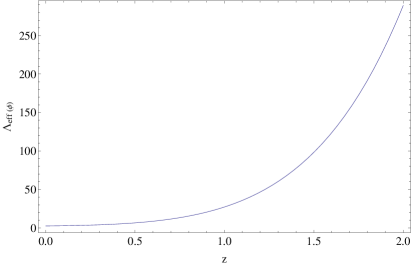
Figure 1: Behaviour of the $\Lambda_{eff}$ term with the redshift (the parameters entering in the model are $\Omega_{m}=0.33$,  $H_{0}=1$,  $\lambda=0.2$

Now in view of equation (13), we get a constant value for $\beta=\beta_{0}$. Equation (15) then yields $\Lambda^{\prime\prime}=0$, ie.,

$$\Lambda=\lambda\phi,$$ (21)

with constant $\lambda$. Thus, in view of Noether symmetry, we have been able to find the functional forms of $\Lambda(\phi)$ and $V(\phi)$ of the model under consideration. It is worth noting that one may always choose $V=V_{0}=\rm{constant}$, a-priori, but choosing a linear form of $\Lambda(\phi)$, without invoking Noether symmetry is highly ambitious. Further, such choices are usually made for mathematical simplicity. We find here that, although apparently simple forms have emerged from Noether symmetry, however, it do not make the field equations tractable to solve directly. It is again interesting to note that, the same form of $\Lambda(\phi)$ was obtained in an earlier work b2 at the late time cosmic evolution, when the kinetic term viz., $\dot{\phi}^{2}$ indeed became constant and the Universe sets off for an accelerated expansion. We just like to mention once again that the coupling parameter and the potential thus found are independent of the evolutionary history of the Universe.

Finally, the point Lagrangian takes the following form,

$$L=-3a\dot{a}^{2}-\lambda\dot{\phi}\dot{a}^{3}+\frac{1}{2}a^{3}\dot{\phi}^{2}-a^{3}V_{0}-M,$$ (22)

which is clearly cyclic in $\phi$. We do not need thus to perform a transformation of variables, as is usually done in Noether symmetry approach e1 . The associated conserved quantity is found quite trivially as

$$n=a^{3}\dot{\phi}-\lambda\dot{a}^{3},$$

which is essentially the generalization of a well known result in the case of constant potential e1 . The field equations now are the following,

$$2\dot{H}+3H^{2}=-\left(\frac{1}{2}\dot{\phi}^{2}-V_{0}+2\lambda\dot{\phi}(H\dot{H}+H^{3})+(\lambda\ddot{\phi})H^{2}\right),$$ (23)

$$3H^{2}=\frac{1}{2}\dot{\phi}^{2}+V_{0}-3\lambda\dot{\phi}H^{3}+\frac{M}{a^{3}},$$ (24)

$$a^{3}\dot{\phi}-\lambda\dot{a}^{3}=n,$$ (25)

However, only two of these are independent and one can utilize the last two for finding explicit solutions of the scale factor and the scalar field, which will finally set the coupling parameter $\Lambda(\phi)$. For this purpose, let us substitute $\dot{\phi}$ from equation (25) in equation (24), to get,

$$3\frac{\dot{a}^{2}}{a^{2}}=-\frac{5}{2}\lambda^{2}\frac{\dot{a}^{6}}{a^{6}}-2\lambda n\frac{\dot{a}^{3}}{a^{6}}+\frac{n^{2}}{2a^{6}}+\frac{M}{a^{3}}+V_{0},$$ (26)

which may be rewritten as,

$$\frac{5}{2}\lambda^{2}\dot{a}^{6}+2\lambda n\dot{a}^{3}+3a^{4}\dot{a}^{2}-V_{0}a^{6}-Ma^{3}-\frac{n^{2}}{2}=0.$$ (27)

This equation is definitely not easy to solve, so in the following section, we take up a different route to analyze the solutions.

II.1 Obtaining solutions

As mentioned, it is clearly not possible to solve analytically equation (27) in order to obtain $a(t)$, but, on the other hand, it turns out to be unnecessary. It can be transformed into an algebraic equation for the Hubble parameter, being interpreted as a function of the red-shift $z$, which is clearly what we need in order to investigate the cosmic evolution in the context of dark energy. Thus, we get,

$$5\lambda^{2}H^{6}+4n\lambda(1+z)^{3}H^{3}+6H^{2}-n^{2}(1+z)^{6}-2M(1+z)^{3}-2V_{0}=0,$$ (28)

where we have set the present value of the scale factor $a_{0}=1$, as usual. The only problem left is the impossibility to get an exact solution of a 6th degree algebraic equation. We must thus give effort to make a reasonable choice of the parameters involved, in order to make a somewhat detailed study of the cosmological consequence of the situation under investigation. Let us stress that, in any case, we are not talking of numerical integration but of simple solution of an algebraic equation.

First, since we want to investigate on acceleration at the present epoch, we need an expression for $H^{\prime}(z)$ (from now on, prime means derivative w.r.t. $z$). Taking derivative of equation (28) it is easy to obtain,

$$H^{\prime}(z)=\frac{6n^{2}(1+z)^{5}+6M(1+z)^{2}-12n\lambda(1+z)^{2}H^{3}}{30\lambda^{2}H^{5}+12n\lambda(1+z)^{3}H^{2}+12H}.$$ (29)

Second, our choice of units leave us free to choose the unit of time. In a recent work, some of us f fixed the present age of the universe $t_{0}=1$. This was due to the fact that, in that case, we had explicit time dependance of the solutions. Here, instead we set the Hubble time to one, i.e., $H_{0}=1$. It should be clear that this does not imply any loss of generality.

Third, we need some “reasonable values” for other parameters. By this we mean to set some parameters of the theory in such a way as to get simple expressions for computations, ending up with a model reasonably similar to the present observable universe, although may not be the best fit. This is due to the fact that for the moment we are mostly interested here to show some important features implied by the introduction of a GB term into the action. A more precise statistical treatment will be given in sec. III.1.

We observe that $M$ parameterizes the amount of matter. In our units it is simply $M=3\Omega_{m0}$. Thus if we assume $\Omega_{m0}=1/3$, we obtain a nice value $M=1$. Since our model is different from $\Lambda$CDM, it is by far not sure that we should obtain the current value of that model, i.e. $\Omega_{m0}=0.26$. This sort of arbitrariness will be fixed later.

The second reasonable choice is to assume that the present value of the deceleration parameter is $q_{0}=-1/2$ (again with some arbitrariness). Hence, finally we are left with

$$V_{0}=2\mp\frac{1}{4}\left(\sqrt{19}\mp 8\right)\lambda^{2}>0\quad\,;\quad n=\mp\frac{1}{2}\left(\sqrt{19}\mp 3\right)\lambda.$$ (30)

We observe that we are finally left with only the $\lambda$ parameter, that will eventually fix up $V_{o}$ and $n$, but with two possible choices, corresponding to two different signs. In the following we will adopt the choice corresponding to the plus signs; however the other one, corresponding to minus signs into equation (30) turns out to be also interesting. Another interesting remark is that $V_{0}$ cannot be zero, attaining a minimum value of 2, for $\lambda=0$. We have also checked that, in general, it is impossible to obtain any acceleration with zero value for $V_{0}$. This means that, actually, it is an effective cosmological constant $\Lambda_{eff(\varphi)}$, which drives the acceleration. Thus one may ask what is the point in setting up all this stuff if the final answer is that we must stay again with the old good $\Lambda$ ? For a possible answer now let us eventually go to some physical quantities.

According to the present choice, we have already fixed $\Omega_{m_{0}}=\frac{1}{3}$, and so are required to compute $\Omega_{\phi 0}$ and $\Omega_{GB0}$. With our choice of parameters we get

$$\Omega_{GB}=-\frac{\lambda(\lambda H^{3}+n/a^{3})}{H^{3}}\quad\,;\quad\Omega_{\varphi}=\frac{2}{3}-\Omega_{GB},$$ (31)

and, substituting $n$ from equation (30) and $H_{0}=a_{0}=1$, we obtain

$$\Omega_{GB0}=\frac{1}{2}\left(\sqrt{19}-5\right)\lambda^{2}\quad\,;\quad\Omega_{\varphi 0}=\frac{1}{6}\left(4-3\left(\sqrt{19}-5\right)\lambda^{2}\right).$$ (32)

Let us remind that $\Omega_{\phi 0}=\rho_{\phi}/(3H_{0}^{2})$ may be interpreted as an effective cosmological constant, so that its evaluation is very important. As $\Omega_{\phi 0}+\Omega_{GB0}=\frac{2}{3}$, there is clearly a degeneration, between $\Omega_{\phi 0}$ and $\Omega_{GB0}$. It is interesting to look at a compared plot of the two.

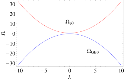
Figure 2: $\Omega_{\varphi 0}$ (upper, red) and $\Omega_{GB0}$(lower, blue) versus $\lambda$. Please note that there is a small gap between the two curves. From text it should be clear that they never sum up to zero

Figure (2) depicts that small values of $\lambda$ takes care of small values of the ”effective cosmological constant”. Instead, large and possibly huge values allow for large (huge) values of it. Thus we see that the presence of the Gauss-Bonnet-dilatonic interaction term $\lambda$ gives us the possibility to reduce the tremendous repulsive power of a large effective cosmological constant $\Lambda_{eff(\varphi)}$. Hence the well known coincidence problem viz., why the cosmological constant is so small today might have been given a plausible answer. This of course is true if all this mechanism gives a good fit with data, which we do just in the next section.

III Comparison with $\Lambda CDM$ and with the observational SnIa data

We are now ready to compare our model with $\Lambda$CDM, to show that they are observationally equivalent, as far as luminosity distance is under consideration. The value of $\lambda$ should be irrelevant in this context. We have checked that it is indeed so, and present a result with $\lambda=0.2$.

Let us consider the standard $\Lambda$CDM expression of the Hubble parameter, normalized to $H_{0}=1$, as mentioned above

$$H_{\Lambda CDM}=\sqrt{\Omega_{\Lambda CDM}(1+z)^{3}+1-\Omega_{\Lambda CDM}},$$ (33)

and compare it with our model. The values for $H$ are obtained by means of numerical solution of equation (28) point by point, with some care in the treatment of the branching points. The best we can do is for $\Omega_{\Lambda CDM}=0.7.$

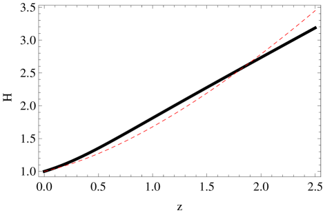
Figure 3: $H_{\Lambda CDM}$ (dotted red line)compared with our model (continuous line). The parameters entering in the model are $\Omega_{m}=0.33$,  $H_{0}=1$,  $\lambda=0.2$

Figure (3) shows that they look rather different. But we know that

$$D_{L}(z)=(1+z)\int_{0}^{z}{\frac{dz^{\prime}}{H(z^{\prime})}},$$

so that the passage to luminosity distance and then to distance modulus act in killing the differences. In our case, the first step is enough. It is possible to compute numerically both luminosity distances and obtain the following plot in Figure (4) which shows that the overlap is perfect, and the slight difference in the values of $\Omega$’s is irrelevant, as mentioned above.

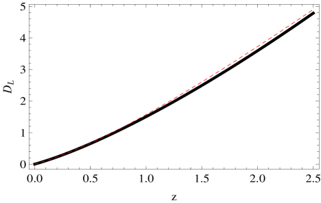
Figure 4: Luminosity distances for $\Lambda$CDM (dotted line), with $\Omega_{\Lambda}=0.73$, and our model (continuous line), with parameters entering $\Omega_{m}=0.33$,  $H_{0}=1$,  $\lambda=0.2$ (corresponding to $\Omega_{\phi_{0}}+\Omega_{{GB}_{0}}=0.67$).

III.1 Constraints from recent SNIa observations

In this subsection we show that our model is compatible with recent observational data, in particular with the observations of type Ia supernovae. We use the most updated SNeIa sample. The present compilation, which is referred to as Union Union2 , includes recent large samples from SNLS SNLS and ESSENCE ESSENCE surveys, older data sets and the recently extended data set of distant SNeIa, observed with HST. All of these have been homogeneously reanalyzed with the same lightcurve fitter. After selection cuts and outliers removal, the final sample contains 557 SNeIa spanning the range $0.015\leq z\leq 1.55$. To constrain our models we actually compare the theoretically   predicted distance modulus $\mu(z)$ with the observed, through a likelihood analysis, where we use as merit function the likelihood $\mathcal{L}=\exp{\left(-\frac{1}{2}\chi^{2}\right)}$. The distance modulus is defined by

$$\mu=m-M=5\log{D_{L}(z)}+5\log({\frac{c}{100h}})+25,$$ (34)

where $m$ is the appropriately corrected apparent magnitude including reddening, K correction etc., $M$ is the corresponding absolute magnitude, $D_{L}$ is the luminosity distance in Mpc, and $h$ is the standard dimensionless Hubble constant. We note that because of our choice of time unit, our Hubble constant is not (numerically) the same as the $\tilde{H}_{0}$ that is usually measured in $\mathrm{kms^{-1}Mpc^{-1}}$. Actually, we may easily obtain the relation

$$h=9.9{\frac{H_{0}}{\tau}}\,,$$ (35)

where as usual $h=\tilde{H}_{0}/100$ and $\tau$ is the age of the universe in Gy, $\tilde{H}_{0.}$ being the Hubble parameter in standard units. We see that $H_{0}$ fixes only the product $h\tau$. In particular, we know that $\tau=13.73_{-0.15}^{+0.16}$ (see for instance WMAP3 ), thus we get $h\leq 0.76$ for $H_{0}\approx 1$. Before going into the details of our statistical analysis thoroughly, it is needed to turn into the parametrization of our solutions, mainly following the Eqs. (30,31,32). Actually, earlier (in the previous subsection), in order to illustrate some basic properties of our model, we fixed the values of $\Omega_{\mathrm{m0}}$, $q_{0}$ ,$H_{0}$ and $\lambda$ also. Here, since we want to constrain the values of the physically meaningful parameters as maximum likelihood ones, comparing theoretical predictions with observational data, we remove the restrictions on the parameters. More generally, indeed

$$\Omega_{\phi_{0}}+\Omega_{{GB}_{0}}=\frac{1}{6}\left[-6H_{0}^{2}(\Omega_{m0}-1)+(H_{0}-1)(H_{0}+1)\left(H_{0}^{2}+H_{0}+1\right)\right.$$

$$\left.(H_{0}(9H_{0}-5)+5)\lambda^{2}-4\left(H_{0}^{3}-1\right)H_{0}^{2}q_{0}\lambda^{2}+\right.$$ (36)

$$\left.-4\left(H_{0}^{3}-1\right)\lambda\sqrt{H_{0}\left(H_{0}^{3}\lambda^{2}\left(H_{0}^{2}-7H_{0}(q_{0}-1)+(q_{0}-1)^{2}\right)-3H_{0}\Omega_{m0}-2q_{0}+2\right)}\right].$$

In fact we have $\Omega_{{\phi}_{0}}+\Omega_{{GB}_{0}}=1-\Omega_{m0}$, as due, in order to satisfy the Einstein equations. If $H_{0}\neq 1$, the previous relation has to be considered as a constraint among the parameters. We actually used it to express $q_{0}$ as function of $H_{0}$, $\Omega_{m0}$ and $\lambda$. The modulus of distance in Eq. (34) turns out to be function of $z$, and $H_{0}$, $\Omega_{m0}$ and $\lambda$. Performing our statistical analysis with the Union2 compilation we marginalize over the $\lambda$ parameter, that is we maximize the likelihood $\mathcal{L}_{marg}=\int_{\lambda_{min}}^{\lambda_{max}}{d\lambda\exp{\left(-\frac{1}{2}\chi^{2}\right)}}$, where $\lambda_{min}$ and $\lambda_{max}$ are fixed by asking that $q_{0}$ should lie in the region allowed by the observations (see for instance daly ). We obtain $\chi_{red}^{2}=0.99$ for 554 points, and the best fit values are $h=0.70_{-0.05}^{+0.03}$, and $\Omega_{\mathrm{m0}}=0.35_{-0.08}^{+0.04}$. In Fig. 5 we compare the best fit curve with the observational dataset. Let us remark that the range of $\Omega_{\mathrm{m0}}$ here obtained, includes the particular value chosen in earlier section. Further, its lower limit is consistent with the presently acceptable value.

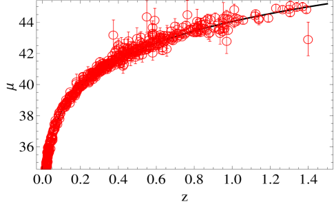
Figure 5: Observational data of the Union2 compilation fitted to our model. The red curve is the best fit curve with $h=0.70_{-0.05}^{+0.03}$, and corresponds to $\Omega_{\mathrm{M0}}=0.35_{-0.08}^{+0.04}$

IV Conclusions

Noether symmetry has been enforced in Gauss-Bonnet dilatonic scalar theory of gravity and the following important results have emerged.

(1)

The coupling parameter and the potential thus found are independent of the evolutionary history of the Universe, ie., Noether symmetry exists throughout the history of evolution of the Universe starting from the early vacuum dominated era, passing over to radiation dominated era and finally at the matter dominated era. Existence of such symmetry fixes up the dilatonic-Gauss-Bonnet coupling parameter $\Lambda=\lambda\phi$ and the scalar potential $V=V_{0}$ (a constant) once and forever.

(2)

The same form of $\Lambda(\phi)$ was obtained in an earlier work b2 at the late time cosmic evolution, when the kinetic term viz., $\dot{\phi}^{2}$ indeed became constant and the Universe sets off for an accelerated expansion.

(3)

Since the potential is obliged to be a constant, the effective cosmological constant is now $\Lambda_{eff}=\Lambda_{eff(\varphi)}+\Lambda_{GB}$, which may be comparable with the present Hubble parameter.

(4)

The late time cosmic acceleration is driven by the scalar field effective cosmological constant rather than the Gauss-Bonnet term.

(5)

Figure (2) depicts that the presence of the Gauss-Bonnet-dilatonic interaction term $\lambda$ puts up the possibility to reduce the tremendous repulsive power of a large effective cosmological constant. Thus the well known coincidence problem viz., why the cosmological constant is so small today might have been given a plausible answer.

(6)

For late universe, there is an almost perfect equivalence with the $\Lambda$CDM model as depicted in Figure (4).

(7)

A more accurate fit procedure gives even more satisfactory results, with a best fit value for $\Omega_{m}$, whose lower limit is consistent with the results obtained from very different kinds of methods using various astronomical objects, within the framework of the standard $\Lambda CDM$ model WMAP3 ; sab .

Acknowledgements:

A.K. Sanyal is grateful to the University of Naples (Ufficio Relazioni Internazionali) for supporting a visit in the Department of Physical Sciences, Naples.

References

References

- (1) S.Kawai and J.Soda, Phys.Lett.B460, 41 (1999).
- (2) G.Esposito-Farese, gr-qc/0306018.
- (3) N.Deruelle and C.Germani, Il Nuovo Cimento. B118, 977 (2003).
- (4) G.Calcagni, S.Tsujikawa and M.Sami, Class.Quant.Gravit.22, 3977 (2005).
- (5) M.Sami et al., Phys.Lett.B619, 193 (2005).
- (6) L.Amendola, C.Charmousis and S.C.Davis, JCAP 10, 004 (2006), hep-th/0506137.
- (7) I.P.Neupane and B.M.N.Carter JCAP06, 004 (2006), hep-th/0512262 and Phys.Lett. B638, 194 (2006), hep-th/0510109.
- (8) S.Nojiri, S.D.Odintsov and M.Sasaki, Phys.Rev.D71, 123509 (2005), hep-th/0504052.
- (9) S.Nojiri and S.D.Odintsov, Phys. Lett.B631, 1 (2005).
- (10) S.Nojiri, S.D.Odintsov and M.Sami, Phys.Rev.D74, 046004 (2006), hep-th/0605039.
- (11) I.P.Neupane, Class.Quant.Grav.23, 7493 (2006), hep-th/0602097 and hep-th/0605265.
- (12) S.Tsujikawa and M. Sami, JCAP01, 006 (2007).
- (13) G.Cognola, E.Elizalde, S.Nojiri, S.D.Odintsov and S.Zerbini, Phys.Rev.D75, 086002 (2007).
- (14) S.Nojiri, S.D.Odintsov and Petr.V.Tretyakov, Phys.Lett.B651 224 (2007), 0704.2520[hep-th].
- (15) A.K.Sanyal, Phys.Lett.B645, 1 (2007), astro-ph/0608104.
- (16) Nojiri, S.; Odintsov, S. D.; (2011) arXiv:1011.0544
- (17) Nojiri, S.; Odintsov, S. D.; (2006), arXiv:hep-th/0601213.
- (18) T.Koivisto and D.F.Mota, Phys.Lett.B644, 104 (2007) and Phys.Rev.D75, 023518 (2007).
- (19) A.K.Sanyal, Gen.Relativ.Gravit.41, 1511 (2009), 0710.2450v2[astro-ph].
- (20) J.Callan et al. Nucl.Phys.B262, 593 (1985).
- (21) D.J.Gross and J.H.Sloan, Nucl.Phys.B291, 41 (1987).
- (22) R.R.Metsaev and A.A.tseytlin, Phys.Lett.B191, 354 (1987).
- (23) M.C.Bento and O.Bertolami, Phys.Lett.B368, 198 (1995).
- (24) R.A.Daly et al., Astrophys.J677, 1 (2008).
- (25) A.K.Sanyal, B.Modak, C.Rubano and E.Piedipalumbo, Gen.Relativ.Grav.37, 407 (2005), astro-ph/0310610.
- (26) S.Capozziello, S.Nesseris and L.Perivolaropoulos, JCAP0712, 009 (2007).
- (27) S.Capozziello, P.Martin-Moruno and C.Rubano, Phys.Lett.B664, 12 (2008), 0804.4340[astro-ph].
- (28) R.de Ritis, G.Marmo, G.Platania, C.Rubano, P.Scudellaro and C.Stornaiolo, Phys.Rev.D42, 1091 (1990) and Phys.Lett.A149, 79 (1990).
- (29) S.Capozziello, R.de Ritis, C.Rubano, and P.Scudellaro, La Rivista del Nuovo Cimento 4, 1 (1996).
- (30) J.E. Lidsey, Class.Quant.Gravit.13, 2449 (1996).
- (31) S.Capozziello, G.Marmo, C.Rubano and P.Scudellaro, Int.J.Mod.PhysD6, 491 (1997).
- (32) C.Rubano and P.Scudellaro, Gen.Relativ.Gravit.34, 307 (2002)
- (33) A.K.Sanyal, Phys.Lett.B524, 177 (2002).
- (34) B.C.Paul and S.Ghose, Gen. Relativ. Grav.42, 795 (2010).
- (35) S.Davis, hep-th/0408138, (2004).
- (36) Elizalde, E.; Jhingan, S.; Nojiri, S.; Odintsov, S. D.; Sami, M.; Thongkool, I. , 2007, arXiv:0705.1211
- (37) M.Demianski, E.Piedipalumbo, C.Rubano and P.Scudellaro, Astron.Astrophys.481, 279 (2008).
- (38) P.Astier, J.Guy, N.Regnault, R.Pain, E.Aubourg et al., Astron.Astrophys.447, 31 (2006).
- (39) W.M.Wood - Vasey, G.Miknaitis, C.W. Stubbs, S.Jha, A.G.Riess et al., Astrophys.J.666, 694 (2007).
- (40) R.Amanullah et al., (The Supernova Cosmology Project), Astrophys.J.716, 712 (2010).
- (41) D.N.Spergel et al., Astrophys.J.(Supp.)170, 377 (2007).
- (42) S.Schindler, Space Science Reviews, 100, 299, (2002).