Optimal Contours for High-Order Derivatives

Abstract.

As a model of more general contour integration problems we consider the numerical calculation of high-order derivatives of holomorphic functions using Cauchy’s integral formula. ? showed that the condition number of the Cauchy integral strongly depends on the chosen contour and solved the problem of minimizing the condition number for circular contours. In this paper we minimize the condition number within the class of grid paths of step size $h$ using Provan’s algorithm for finding a shortest enclosing walk in weighted graphs embedded in the plane. Numerical examples show that optimal grid paths yield small condition numbers even in those cases where circular contours are known to be of limited use, such as for functions with branch-cut singularities.

1. Introduction

To escape from the ill-conditioning of difference schemes for the numerical calculation of high-order derivatives, numerical quadrature applied to Cauchy’s integral formula has on various occasions been suggested as a remedy (for a survey of the literature, see ?). To be specific, we consider a function $f$ that is holomorphic on a complex domain $D\ni 0$; Cauchy’s formula gives

$$f^{(n)}(0)=\frac{n!}{2\pi i}\int_{\Gamma}z^{-n-1}f(z)\,dz$$ (1)

for each cycle $\Gamma\subset D$ that has winding number $\operatorname{ind}(\Gamma;0)=1$. If $\Gamma$ is not carefully chosen, however, the integrand tends to oscillate at a frequency of order $O(n^{-1})$ with very large amplitude (?, Fig. 4). Hence, in general, there is much cancelation in the evaluation of the integral and ill-conditioning returns through the backdoor. The condition number of the integral is (?, Lemma 9.1)

$$\kappa(\Gamma,n)=\frac{\int_{\Gamma}|z|^{-n-1}|f(z)|\,d|z|}{\left|\int_{\Gamma}z^{-n-1}f(z)\,dz\right|}$$

and $\Gamma$ should be chosen as to make this number as small as possible. Equivalently, since the denominator is, by Cauchy’s theorem, independent of $\Gamma$, we have to minimize

$$d(\Gamma)=\int_{\Gamma}|z|^{-n-1}|f(z)|\,d|z|.$$ (2)

? considered circular contours of radius $r$; he found that there is a unique $r_{*}=r(n)$ solving the minimization problem and that there are different scenarios for the corresponding condition number $\kappa_{*}(n)$ as $n\to\infty$:

• $\kappa_{*}(n)\to\infty$, if $f$ is in the Hardy space $H^{1}$;
  

• $\limsup_{n\to\infty}\kappa_{*}(n)\leqslant M$, if $f$ is an entire function of completely regular growth which satisfies a non-resonance condition of the zeros and whose Phragmén–Lindelöf indicator possesses $M$ maxima (a small integer).

Hence, though those (and similar) results basically solve the problem of choosing proper contours for entire functions, much better contours have to be found for the class $H^{1}$. Moreover, the restriction to circles lacks any algorithmic flavor that would point to more general problems depending on the choice of contours, such as the numerical solution of highly-oscillatory Riemann–Hilbert problems (?).

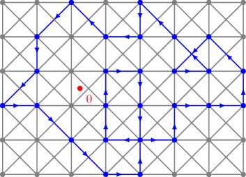
Figure 1. Path $\Gamma$ with $\operatorname{ind}(\Gamma;0)=1$ in a grid-graph of step size $h$.

In this paper, we solve the contour optimization problem within the more general class of grid paths of step size $h$ (see Fig. 1; we allow diagonals to be included) as they are known from Artin’s proof of the general, homological version of Cauchy’s integral theorem (?, IV.3). Such paths are composed from horizontal, vertical and diagonal edges taken from a (bounded) grid $\Omega_{h}\subset D$ of step size $h$. Now, the weight function (2), being additive on the abelian group of path chains, turns the grid $\Omega_{h}$ into an edge-weighted graph such that each optimal grid path $W_{*}$ becomes a shortest enclosing walk (SEW); “enclosing” because we have to match the winding number condition $\operatorname{ind}(W_{*};0)=1$. An efficient solution of the SEW problem for embedded graphs was found by ? and serves as a starting point for our work.

Outline of the Paper

In Section 2 we discuss general embedded graphs in which an optimal contour is to be searched for; we discuss the problem of finding a shortest enclosing walk and recall Provan’s algorithm. In Section 3 we discuss some implementation details and tweaks for the problem at hand. Finally, in Section 4 we give some numerical examples; these can easily be constructed in a way that the new algorithm outperforms, by orders of magnitude, the optimal circles of ? with respect to accuracy and the direct symbolic differentiation with respect to efficiency.

2. Contour Graphs and Shortest Enclosing Walks

By generalizing the grid $\Omega_{h}$, we consider a finite graph $G=(V,E)$ embedded to $D$, that is, built from vertices $V\subset D$ and edges $E$ that are smooth curves connecting the vertices within the domain $D$. We write $uv$ for the edge connecting the vertices $u$ and $v$; by (2), its weight is defined as

$$d(uv)=\int_{uv}|z|^{-n-1}|f(z)|\,d|z|.$$ (3)

A walk $W$ in the graph $G$ is a closed path built from a sequence of adjacent edges, written as (where $\operatorname{\dot{+}}$ denotes joining of paths)

$$W=v_{1}v_{2}\operatorname{\dot{+}}v_{2}v_{3}\operatorname{\dot{+}}\cdots\operatorname{\dot{+}}v_{m}v_{1};$$

it is called enclosing the obstacle $0$ if the winding number is $\operatorname{ind}(W;0)=1$. The set of all possible enclosing walks is denoted by $\Pi$. As discussed in §1, the condition number is optimized by the shortest enclosing walk (not necessarily unique)

$$W_{*}=\operatorname*{argmin}_{W\in\Pi}d(W)$$

where, with $W=v_{1}v_{2}\operatorname{\dot{+}}v_{2}v_{3}\operatorname{\dot{+}}\cdots\operatorname{\dot{+}}v_{m}v_{1}$ and $v_{m+1}=v_{1}$, the total weight is

$$d(W)=\sum_{j=1}^{m}d(v_{j}v_{j+1}).$$

The problem of finding such a SEW was solved by ?: the idea is that with $\mathcal{P}_{u,v}$ denoting a shortest path between $u$ and $v$, any shortest enclosing walk $W_{*}=w_{1}w_{2}\operatorname{\dot{+}}w_{2}w_{3}\operatorname{\dot{+}}\cdots\operatorname{\dot{+}}w_{m}w_{1}$ can be cast in the form (?, Thm. 1)

$$W_{*}=\mathcal{P}_{w_{1},w_{j}}\operatorname{\dot{+}}w_{j}w_{j+1}\operatorname{\dot{+}}\mathcal{P}_{w_{j+1},w_{1}}$$

for at least one $j$. Hence, any shortest enclosing walk $W_{*}$ is already specified by one of its vertices and one of its edges; therefore

$$W_{*}\in\tilde{\Pi}=\{\mathcal{P}_{u,v}\operatorname{\dot{+}}vw\operatorname{\dot{+}}\mathcal{P}_{w,u}:u\in V,vw\in E\}.$$

Provan’s algorithm finds $W_{*}$ by, first, building the finite set $\tilde{\Pi}$; second, by removing all walks from it that do not enclose $z=0$; and third, by selecting a walk from the remaining candidates that has the lowest total weight. Using ? implementation of Dijkstra’s algorithm to compute the shortest paths $\mathcal{P}_{u,v}$, the run time of the algorithm is known to be (?, Corollary 2)

$$O(|V|\,|E|+|V|^{2}\log|V|).$$ (4)

3. Implementation Details

We restrict ourselves to graphs $\Omega_{h}$ given by finite square grids of step size $h$, centered at $z=0$—with all vertices and edges removed that do not belong to the domain $D$. Since Provan’s algorithm just requires an embedded graph but not a planar graph, we may add the diagonals of the grid cells as further edges to the graph (see Fig. 1). For such a graph $\Omega_{h}$, with or without diagonals, we have $|V|=O(h^{-2})$ and $|E|=O(h^{-2})$ so that the complexity bound (4) simplifies to

$$O(h^{-4}\log h^{-1}).$$

3.1. Edge Weight Calculation

Using the edge weights $d(uv)$ on $\Omega_{h}$ requires to approximate the integral in (3). Since not much accuracy is needed here, a simple trapezoidal rule with two nodes is generally sufficient:

$$d(uv) =\int_{uv}|z|^{-(n+1)}|f(z)|d|z|$$

$$=\frac{|u-v|}{2}\left(d(u)+d(v)\right)+O(h^{3})=\tilde{d}(uv)+O(h^{3})$$

with the vertex weight

$$d(z)=|z|^{-(n+1)}|f(z)|.$$ (5)

Although $\tilde{d}(uv)$ will typically have an accuracy of not more than just a few bits for the rather coarse grids $\Omega_{h}$ we work with, we have not encountered a single case in which a more accurate computation of the weights would have resulted in a different SEW $W_{*}$.

$\operatorname{Ai}(z)$

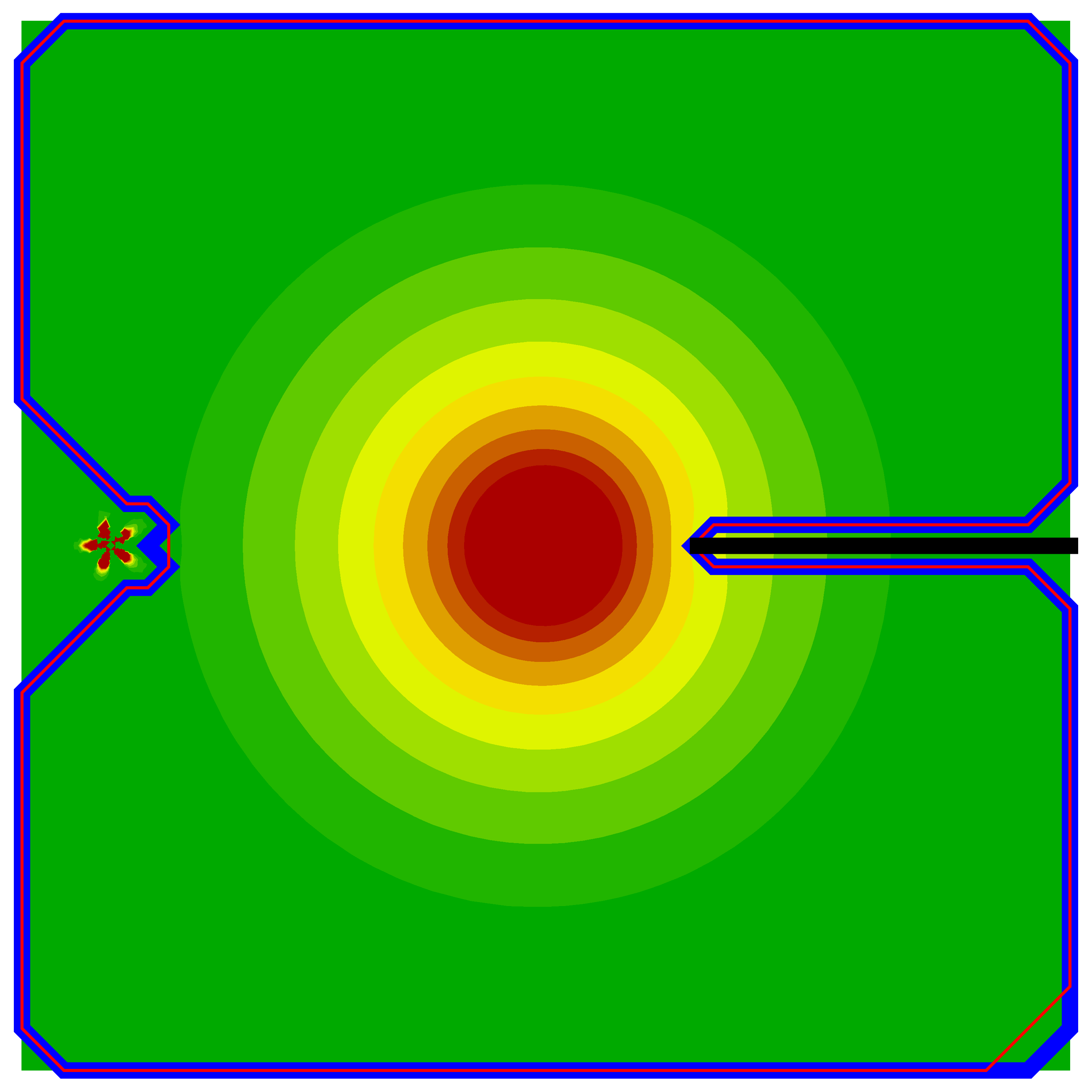
$\exp(1/(1+8z)^{1/5})(1-z)^{11/2}J_{0}(z)$

Figure 2. $W_{*}$ (red) vs. $W_{v_{*}}$ (blue): the color coding shows the size of $\log d(z)$; with red for large values and green for small values. The smallest level shown is the threshold, below of which the edges of $W_{*}$ do not contribute to the first couple of significant digits of the total weight. The plots illustrate that $W_{*}$ and $W_{v_{*}}$ differ typically just in a small region well below this threshold; consequently, both walks yield about the same condition number. On the right note the five-leaved clover that represents the combination of algebraic and essential singularity at $z=-1$.

3.2. Reducing the size of $\tilde{\Pi}$

As described in Section 2, Provan’s algorithm starts by building a walk for every pair $(v,e)\in V\times E$ and then proceeds by selecting the best enclosing one. A simple heuristic, which worked well for all our test cases, helps to considerably reduce the number of walks to be processed: Let

$$v_{*}=\underset{v\in V}{\operatorname*{argmin}}\,d(v)\\$$

and define $W_{v_{*}}$ as a SEW subject to the constraint

$$W_{v_{*}}\in\tilde{\Pi}_{v_{*}}=\{\mathcal{P}_{v_{*},u}\operatorname{\dot{+}}uw\operatorname{\dot{+}}\mathcal{P}_{w,v_{*}}:uw\in E\}.$$

Obviously $W_{*}$ and $W_{v_{*}}$ do not need to agree in general, as $v_{*}$ does not have to be traversed by $W_{*}$. However, since $v_{*}$ is the vertex with lowest weight, both walks differ mainly in a region that has no, or very minor, influence on the total weight and, consequently, also no significant influence on the condition number. Actually, $W_{*}$ and $W_{v_{*}}$ yielded precisely the same total weight for all functions that we have studied (Fig. 2 compares $W_{*}$ and $W_{v_{*}}$ for two typical examples). Using that heuristic, the run time of Provan’s algorithm improves to $O(|E|+|V|\log|V|)$ because its main part reduces to applying Dijkstra’s shortest path algorithm just once. In the case of the grid $\Omega_{h}$ this bound simplifies to

$$O(h^{-2}\log h^{-1}).$$

3.3. Size of the Grid Domain

The side length $l$ of the square domain supporting $\Omega_{h}$ has to be chosen large enough to contain a SEW that would approximate an optimal general integration contour. E.g., if $f$ is entire, we choose $l$ large enough for this square domain to cover the optimal circular contour: $l>2r_{*}$, where $r_{*}$ is the optimal radius given in ?; a particularly simple choice is $l=3r_{*}$. In other cases we employ a simple search for a suitable value of $l$ by calculating $W_{*}$ for increasing values of $l$ until $d(W_{*})$ does not decrease substantially anymore. During this search the grid will be just rescaled, that is, each grid uses a fixed number of vertices; this way only the number of search steps enters as an additional factor in the complexity bound.

3.4. Multilevel Refinement of the SEW

Choosing a proper value of $h$ is not straightforward since we would like to balance a good approximation of a generally optimal integration contour with a reasonable amount of computing time. In principle, we would construct a sequence of SEWs for smaller and smaller values of $h$ until the total weight of $W_{*}$ does not substantially decrease anymore. To avoid an undue amount of computational work, we do not refine the grid everywhere but use an adaptive refinement by confining it to a tubular neighborhood of the currently given SEW $W_{*}$ (see Fig. 3):

• calculate $W_{*}$ within an initial grid;
  

• subdivide each rectangle adjacent to $W_{*}$ into 4 rectangles;
  

• remove all other rectangles;
  

• calculate $W_{*}$ in the newly created graph.

As long as the total weight of $W_{*}$ decreases substantially, steps 2 to 4 are repeated. It is even possible to tweak that process further by not subdividing rectangles that just contain vertices or edges of $W_{*}$ having weights below a certain threshold. By geometric summation, the complexity of the resulting algorithm is

$$O(H^{-4}\log{H^{-1}})+O(h^{-2}\log{h^{-1}})$$

where $H$ denotes the step size of the coarsest grid and $h=H/2^{k}$ the step size after $k$ loops of adaptive refinement. An analogous approach to the constrained $W_{v_{*}}$-variant of the SEW algorithm given in §3.2 reduces the complexity further to

$$O(H^{-2}\log{H^{-1}})+O(h^{-1}\log{h^{-1}}),$$

which is close to the best possible bound $O(h^{-1})$ given by the work that would be needed to just list the SEW.

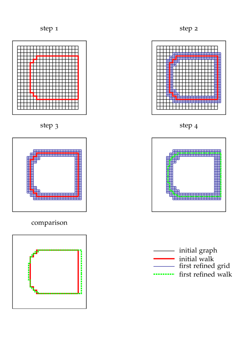
Figure 3. Multilevel refinement of $W_{*}$ $(f(z)=1/\Gamma(z),\,n=2006)$

3.5. Quadrature Rule for the Cauchy Integral

Finally, after calculation of the SEW $\Gamma=W_{*}$, the Cauchy integral (1) has to be evaluated by some accurate numerical quadrature. We decompose $\Gamma$ into maximally straight line segments, each of which can be a collection of many edges. On each of those line segments we employ Clenshaw–Curtis quadrature in Chebyshev–Lobatto points. Additionally we neglect segments with a weight smaller than $10^{-24}$ times the maximum weight of an edge of $\Gamma$, since such segments will not contribute to the result within machine precision. This way we not only get spectral accuracy but also, in many cases, less nodes as would be needed by the vanilla version of trapezoidal sums on a circular contour: Fig. 4 shows an example with the order $n=300$ of differentiation but accurate solutions using just about $200$ nodes which is well below what the sampling condition would require for circular contours (?, §2.1). Of course, trapezoidal sums would also benefit from some recursive device that helps to neglect those nodes which do not contribute to the numerical result.

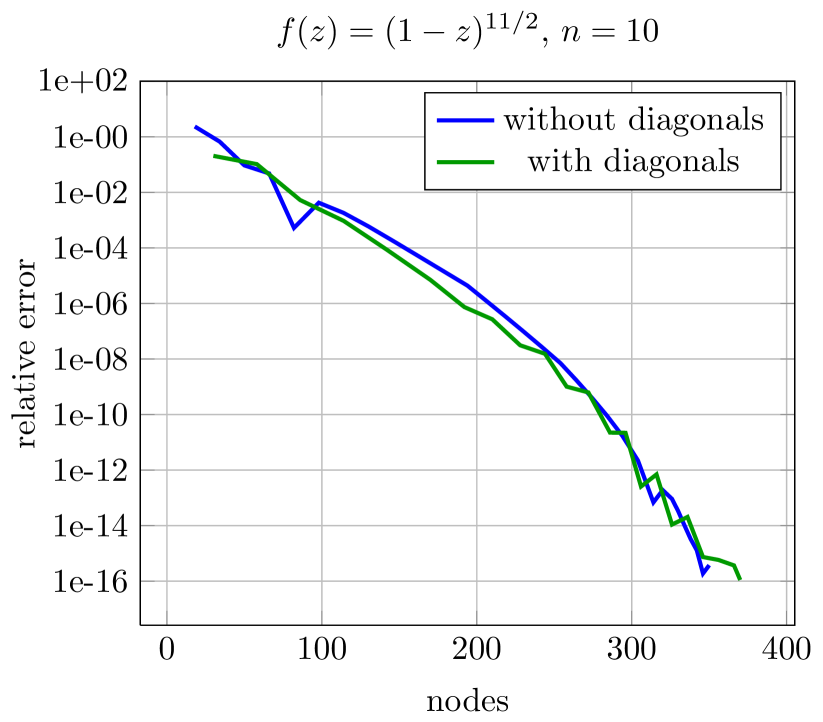
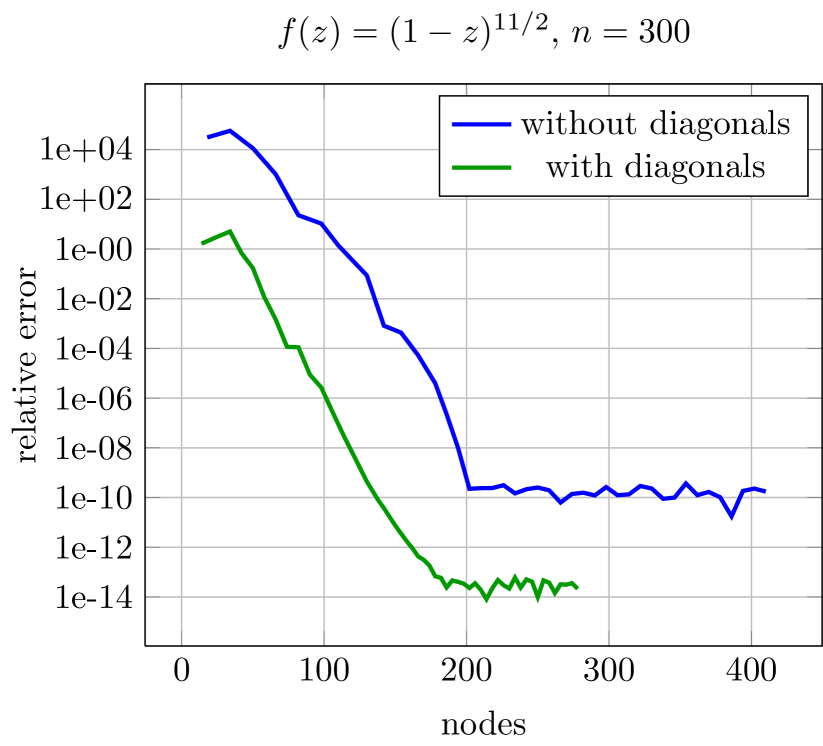
Figure 4. Illustration of the spectral accuracy of piecewise Clenshaw–Curtis quadrature on SEW contours for a function with a branch-cut singularity. For larger $n$, we observe a significant improvement by adding diagonals to the grid. We get to machine precision for $n=10$ and loose about two digits for $n=300$. (Note that for optimized circular contours the loss would have been about 6 digits for $n=10$ and about 15 digits for $n=300$; cf. Bornemann 2011, Thm. 4.7).

Table 1. Condition numbers for some $f(z)$: $r_{*}$ are the optimal radii given in ?; $W_{*}$ was calculated in all cases on a $51\times 51$-grid with $l=3r_{*}$ (in the last two cases $l$ was found as in §3.3). For $1/\Gamma(z)$, the peculiar order of differentiation $n=2006$ is one of the very rare resonant cases (specific to this entire function) for which circles give exceptionally large condition numbers (cf. ?, Table 5). In the last example, differentiation is for $z=1/\sqrt{2}$.

$f(z)$ $n$ $\kappa(W_{*},n)$ $\kappa(C_{r_{*}},n)$ $e^{z}$ $300$ $1.1$ $1.0$ $\operatorname{Ai}(z)$ $300$ $1.3$ $1.2$ $1/\Gamma(z)$ $300$ $1.7$ $1.6$ $1/\Gamma(z)$ $2006$ $7.8\cdot 10^{4}$ $4.7\cdot 10^{4}$ $(1-z)^{11/2}$ $10$ $1.4$ $5.0\cdot 10^{5}$ $\exp(1/(1+8z)^{1/5})(1-z)^{11/2}J_{0}(z)$ $100$ $7.2\cdot 10^{2}$ $4.3\cdot 10^{12}$

Table 2. CPU times for the examples of Table 1. Here $t_{W_{*}}$ and $t_{W_{v_{*}}}$ denote the times to compute $W_{*}$ and $W_{v_{*}}$ and $t_{\text{quad}}$ denotes the time to approximate the integral (1) on such a contour by quadrature. (There is no difference between $W_{*}$ and $W_{v_{*}}$ from the point of quadrature, see Fig. 2.) In the last example, differentiation is for $z=1/\sqrt{2}$. The timings for the grids of size $25\times 25$ and $51\times 51$ match nicely the $O(h^{-4}\log h^{-1})$ complexity for $W_{*}$ and the $O(h^{-2}\log h^{-1})$ complexity for $W_{v_{*}}$.

$f(z)$ $n$ grid $t_{W_{*}}$ $t_{W_{v_{*}}}$ $t_{\text{quad}}$ $e^{z}$ $300$ $51\times 51$ $4.4\cdot 10^{2}$ s $1.5$ s $0.3$ s $\operatorname{Ai}(z)$ $300$ $25\times 25$ $2.1\cdot 10^{1}$ s $0.5$ s $1.7$ s $\operatorname{Ai}(z)$ $300$ $51\times 51$ $4.0\cdot 10^{2}$ s $2.1$ s $2.1$ s $1/\Gamma(z)$ $300$ $25\times 25$ $2.0\cdot 10^{1}$ s $0.5$ s $1.5$ s $1/\Gamma(z)$ $300$ $51\times 51$ $3.6\cdot 10^{2}$ s $2.4$ s $1.3$ s $1/\Gamma(z)$ $2006$ $51\times 51$ $3.6\cdot 10^{2}$ s $2.3$ s $3.1$ s $(1-z)^{11/2}$ $10$ $51\times 51$ $1.4\cdot 10^{3}$ s $5.9$ s $0.2$ s $\exp(1/(1+8z)^{1/5})(1-z)^{11/2}J_{0}(z)$ $100$ $51\times 51$ $7.0\cdot 10^{2}$ s $3.5$ s $0.3$ s

$\operatorname{Ai}(z)$

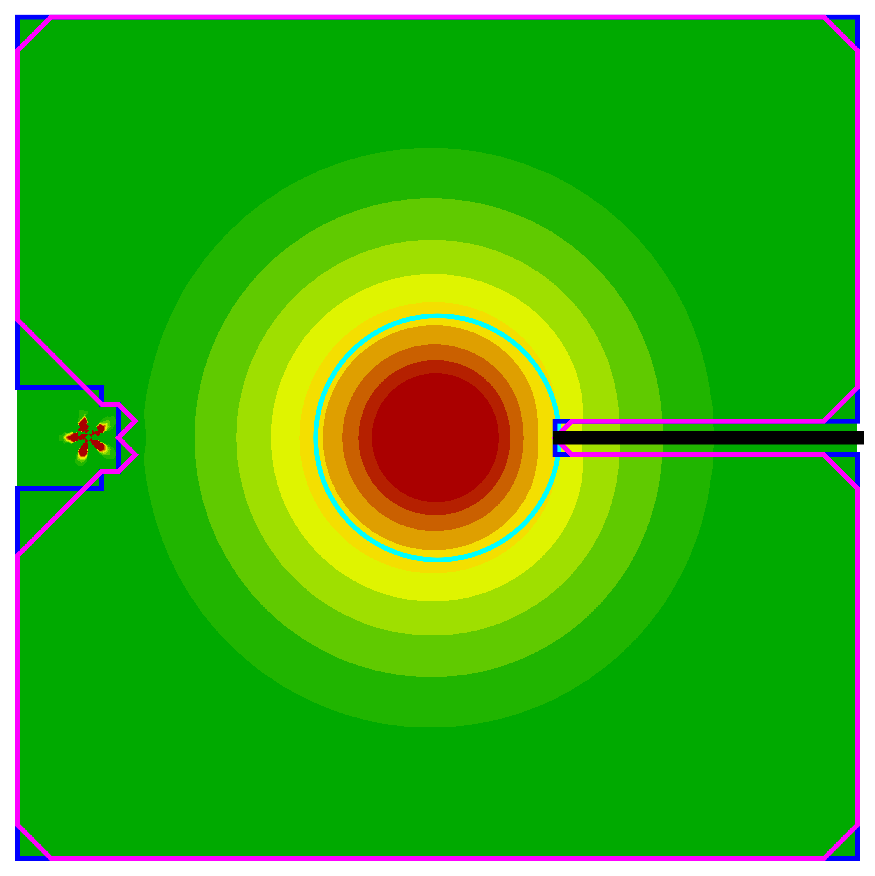
$\exp(1/(1+8z)^{1/5})(1-z)^{11/2}J_{0}(z)$

Figure 5. $W_{v_{*}}$ (blue: $\Omega_{h}$ without diagonals, magenta: $\Omega_{h}$ with diagonals) vs. $C_{r_{*}}$ (cyan) for some examples of Table 1: the color coding shows the size of $\log d(z)$; with red for large values and green for small values. The smallest level shown is the threshold, below of which the edges of $W_{v_{*}}$ do not contribute to the first significant digits of the total weight.

4. Numerical Results

Table 1 displays condition numbers of SEWs $W_{*}$ as compared to the optimal circles $C_{r_{*}}$ for five functions; Table 2 gives the corresponding CPU times and Fig. 5 shows some of the contours. (All experiments were done using hardware arithmetic.) The purpose of these examples is twofold, namely to demonstrate that:

1. the SEW algorithm matches the quality of circular contours in cases where the latter are known to be optimal such as for entire functions;

2. the SEW algorithm is significantly better than the circular contours in cases where the latter are known to have severe difficulties.

Thus, the SEW algorithm is a flexible automatic tool that covers various classes of holomorphic functions in a completely algorithmic fashion; in particular there is no deep theory needed to just let the computation run.

In the examples of entire $f$ we observe that $W_{*}$ and $W_{v_{*}}$, like the optimal circle $C_{r_{*}}$ would do, traverses the saddle points of $d(z)$. It was shown in ? that, for such $f$, the major contribution of the condition number comes from these saddle points and that circles are (asymptotically, as $n\to\infty$) paths of steepest decent. Since $W_{*}$ can cross a saddle point only in a horizontal, vertical, or (if enabled) diagonal direction, somewhat larger condition numbers have to be expected. However, the order of magnitude of the condition number of $C_{r_{*}}$ is precisely matched. This match holds in cases where circles give a condition number of approximately $1$, as well as in cases with exceptionally large condition numbers, such as for $f(z)=1/\Gamma(z)$ in the peculiar case of the order of differentiation $n=2006$ (cf. ?, §10.4).

For non-entire $f$, however, optimized circles will be far from optimal in general: ? shows that the optimized circle $C_{r_{*}}$ for functions $f$ from the Hardy space $H^{1}$ with boundary values in $C^{k,\alpha}$ yields a lower condition number bound of the form

$$\kappa(C_{r_{*}},n)\geqslant cn^{k+\alpha};$$

for instance, $f(z)=(1-z)^{11/2}$ gives $\kappa(C_{r_{*}},n)\sim 0.16059\cdot n^{13/2}$. On the other hand, $W_{*}$ gives condition numbers that are orders of magnitude better than those of $C_{r_{*}}$ by automatically following the branch cut at $(1,\infty)$.

The latter example can easily be cooked-up to outperform symbolic differentiation as well: using Mathematica 8, the calculation of the $n$-th derivative of $f(z)=\exp(1/(1+8z)^{1/5})(1-z)^{11/2}J_{0}(z)$ at $z=1/\sqrt{2}$ takes already about a minute for $n=23$ but had to be stopped after more than a week for $n=100$. Despite the additional difficulty stemming from the combination of an algebraic and an essential singularity at $z=-1$, the $W_{v_{*}}$ version of the SEW calculates this $n=100$ derivative to an accuracy of 13 digits in less than $4\,$s; whereas optimized circular contours would give only about 3 correct digits here (see Fig. 6).

While many more such numerical experiments would demonstrate that reasonably small condition numbers are obtainable in general, the study of rigorous condition number bounds for the SEW has to be postponed to future work.

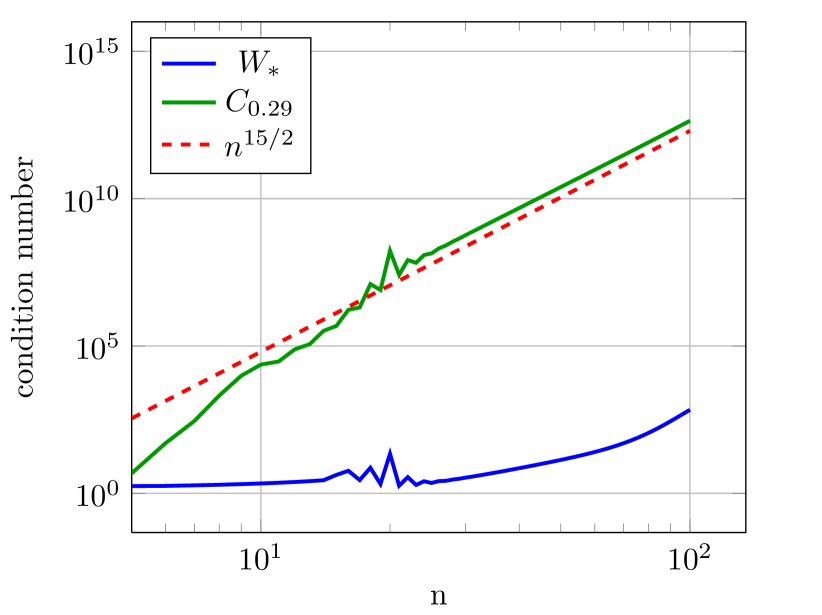
Figure 6. An example with essential and algebraic singularities: the condition number of the Cauchy integral for $\exp(1/(1+8z)^{1/5})(1-z)^{11/2}J_{0}(z)$ for varying order $n$ of differentiation at $z=1/\sqrt{2}$; blue: optimal contour $W_{*}$ in a $51\times 51$ grid graph; green: circular contour with near optimal radius $r=0.29\approx 1-1/\sqrt{2}$; red: prediction of the growth rate from ?.