The resonant nonlinear scattering theory with bound states in the radiation continuum and the second harmonic generation

Abstract

A nonlinear electromagnetic scattering problem is studied in the presence of bound states in the radiation continuum. It is shown that the solution is not analytic in the nonlinear susceptibility and the conventional perturbation theory fails. A non-perturbative approach is proposed and applied to the system of two parallel periodic arrays of dielectric cylinders with a second order nonlinear susceptibility. This scattering system is known to have bound states in the radiation continuum. In particular, it is demonstrated that, for a wide range of values of the nonlinear susceptibility, the conversion rate of the incident fundamental harmonic into the second one can be as high as 40% when the distance between the arrays is as low as a half of the incident radiation wavelength. The effect is solely attributed to the presence of bound states in the radiation continuum.

I Introduction

A conventional approach to nonlinear electromagnetic scattering problems is based on the power series expansion in a nonlinear susceptibility $\chi_{c}$. For example, for the 2nd order susceptibility, the physical parameter that determines nonlinear effects is $\chi_{c}E_{r}\ll 1$ where $E_{r}$ is the electric field at the scattering structure. The smallness of $\chi_{c}E_{r}$ justifies the use of perturbation theory and the solution is analytic in $\chi_{c}$. The situation is different if the scattering structure has resonances.

Planar periodic structures (e.g., gratings) are known to exhibit sharp scattering resonances when illuminated by electromagnetic waves (for a review see, e.g., abajo ; b17 ). Furthermore, it is known (see, e.g., b17 ) that in such structures a local electromagnetic field $E_{r}$ is amplified if the structure has narrow resonances: $E_{r}\sim E_{i}/\sqrt{\Gamma}$, where $E_{i}$ is the amplitude of the incident wave and $\Gamma$ is the width of the resonance. Consequently, optical nonlinear effects are amplified if the system has a sufficiently narrow resonance. For example, an amplification of the second harmonics generation by a single periodic array of dielectric cylinders b23 and by other single-array periodic systems shg have been reported, but no significant flux conversion rate, comparable to that in conventional methods of second harmonic generation, has been found. Owing to the smallness of $\chi_{c}$ and a finite $1/\sqrt{\Gamma}$, the condition $\chi_{c}E_{r}\ll 1$ still holds for the studied structures.

If two identical planar periodic structures are aligned parallel and separated by a distance $2h$, then it can be shown that for each resonance associated with the single structure, the combined structure has two close resonances whose width depends continuously on $h$ so that the width of one of the resonances vanishes, i.e., $\Gamma(h)\rightarrow 0$ as $h\rightarrow h_{b}$ for some discrete set of distances $h_{b}$, for sufficiently large $h$  svs0 ; b17 ; jmp . This means that the system has bound states in the radiation continuum. Their existence was first predicted in quantum mechanics by von Neumann and Wigner b1 in 1929 and later they were discovered in some atomic systems b3 (see also b5 ; b6 ; b7 for more theoretical studies). Their analog in Maxwell’s theory has only attracted attention recently svs0 ; bsp1 ; bsp2 ; bsp3 . In particular, for a system of two parallel arrays of periodically positioned subwavelength dielectric cylinders (depicted in Panel (a) of Fig. 1), the existence of bound states in the radiation continuum has been first established in numerical studies of the system svs0 . A complete classification of bound states as well as their analytic form for this system is given in jmp for TM polarization. It is also shown jmp that bound states exist in the spectral range in which more than one diffraction channel are open. From the physical point of view, bound states in the radiation continuum are localized solutions of Maxwell’s equations like waveguide modes, but in contrast to the latter their spectrum lies in the spectrum of scattering radiation (diffraction) modes.

The perturbation theory parameter $\chi_{c}E_{r}\sim\chi_{c}E_{i}/\sqrt{\Gamma(h)}$, as defined above, can no longer be considered small if bound states in the radiation continuum are present. This qualitative assessment should be taken with a precaution. In the present study, a rigorous analysis of the nonlinear scattering problem by means of the formalism of Siegert states (appropriately extended to periodic structures rs2 ) shows that no divergence of a local field occurs as $h\rightarrow h_{b}$. However, the conventional perturbative approach fails because the solution is not analytic in $\chi_{c}$. The situation can be compared with a simple mechanical analog. Consider a scattering problem for a particle on a line in a hard core repulsive potential $V(x)=g/x^{2}$, $g>0$. No matter how small $g$ is, the particle never crosses the origin $x=0$ and a full reflection occurs, but it does so when $g=0$ (a full transmission). So, the scattering amplitude is not analytic in $g$. Other, more sophisticated, examples of quantum systems with such properties are studied in klauder .

The purpose of the present study is twofold. First, the nonlinear scattering problem is studied in the presence of bound states in the radiation continuum. A non-perturbative approach is developed to solve the problem. Second, as an application of the developed formalism, the problem of the second harmonic generation is analyzed with an example of the system depicted in Fig. 1 (Panel (a)).

I.1 An overview of the results

In Section II, the nonlinear resonant scattering problem with bound states in the radiation continuum is transformed into a system of integral equations. A non-perturbative method is proposed to solve these equations in the approximation that takes into account two nonlinear effects: a second harmonic generation in the leading order of $\chi_{c}$, and the fundamental harmonic generation by mixing the second and fundamental harmonics in the leading order in $\chi_{c}$. This is the second order effect in $\chi_{c}$ known in the theory as the optical rectification. The latter is shown to be necessary to ensure the energy flux conservation.

The formalism is illustrated with an example of two parallel periodic arrays of dielectric cylinders shown in Panel (a) of Fig. 1. The analysis is based on the subwavelength approximation (Section III) when the incident wave length is larger than the radius $R$ of the cylinders. If $k$ is the magnitude of the wave vector, then the theory has three small parameters:

$$\delta_{0}(k)={\textstyle\frac{1}{4}}\,(kR)^{2}(\varepsilon_{c}-1)\ll 1\,,\ \ \ \chi_{c}\ll 1\,,\ \ \ |\Delta h|=|h-h_{b}|\ll 1$$

where all the distances are measured in units of the structure period, in particular $R<1/2$. $\delta_{0}(k)$ is the scattering phase for a single cylinder, $\varepsilon_{c}$ is the linear dielectric susceptibility, and the amplitude of the incident wave is set to one, $E_{i}=1$. With this choice of units, all three parameters are dimensionless. The scattering amplitudes of the fundamental and second harmonics are explicitly found in Section IV.

In Section V, it is shown that the ratio of the flux of the second harmonic along the normal direction and the incident flux is

$$\sigma_{2}=C\chi_{c}^{2}E_{r}^{4}$$

where $E_{r}=E_{r}(\chi_{c},\Delta h,\delta_{0})$ is the fundamental field on the cylinders, and $C=C(\delta_{0},\Delta h)$ is some function. The function $E_{r}$ is non-analytic in the vicinity of zero values of its arguments. The non-perturbative approach of Section II is used to prove that the generated flux of the second harmonic attains its maximal value when the small parameters satisfy the condition

$$(\Delta h)^{4}\delta_{0}^{3}(k_{b})=\vartheta\,\chi_{c}^{2}$$ (1)

where $\vartheta\ll 1$ is a numerical constant, and $k_{b}$ is the magnitude of the wave vector of the bound state that occurs at $h=h_{b}$. Under this condition, $\sigma_{2}$ becomes analytic in the scattering phase $\delta_{0}$ so that in the leading order,

$$\sigma_{2,{\rm max}}\approx 4\pi k_{b}^{-1}\delta_{0}(k_{b})$$

An interesting feature to note is the independence of the conversion efficiency on the nonlinear susceptibility $\chi_{c}$ (in the leading order in the scattering phase $\delta_{0}$). In other words, given a nonlinear susceptibility $\chi_{c}$, by a fine tuning of the distance between the arrays one can always reach the maximal value which is only determined by the scattering phase at the wave length of a bound state. The lowest value of $k_{b}$ for the system considered occurs just below the first diffraction threshold (the wavelength is slightly larger than the structure period) jmp , i.e., $k_{b}\approx 2\pi$. Taking, for example, $R=0.15$ and $\varepsilon_{c}=2$ (so that $\delta_{0}(2\pi)\approx 0.22$), the conversion rate reads $\sigma_{2,{\rm max}}\approx 0.44$, that is, about $44\%$ of the incident flux is converted into the second harmonic flux, which is comparable with the conversion rate achieved in slabs (crystals) of optical nonlinear materials crystals .

From the physical point of view, the scattering structure plays the role of a resonator with the quality factor inversely proportional to $\Gamma$. The field in the resonator is not uniform and has periodic peaks of the amplitude $E_{r}\sim E_{i}/\sqrt{\Gamma}$ due to a constructive interference of the scattered fundamental harmonic. The second harmonic is produced by the induced dipole radiation of point scatters located at these peaks. The induced dipole strength is proportional to $\chi_{c}E_{r}^{2}$. The dipoles are excited by the incident wave and, due to their periodic arrangement, they radiate in phase producing a plane wave in the asymptotic region (just like a phased array antenna). If the system has a resonance whose width $\Gamma$ can be continuously driven to zero by changing a physical parameter of the system, i.e., the system has a bound state in the radiation continuum, then the strength of the induced dipoles radiating the second harmonics can be magnified as desired, but the resonator cannot be excited by the incident radiation if $\Gamma=0$ (a bound state is decoupled from the radiation continuum). So, the optimal width $\Gamma$ at which the second harmonic amplitude is maximal occurs for some $\Gamma\neq 0$, which explains the existence of conditions like (1). Since the second harmonic is generated by point scatterers, the phase matching condition, needed for optically nonlinear crystals, is not required. The energy flux of the incident radiation is automatically redistributed and focused on the scatterers owing to the constructive interference. Thanks to these physical features, an active length at which the conversion rate is maximal is close to $2h_{b}$ whose smallest value for the system studied is roughly a half of the wave length of the incident light svs0 ; jmp (i.e. for an infrared incident radiation it is about a few hundreds nanometers).

II The nonlinear resonant scattering theory

Suppose that a scattering system has a translational symmetry along a particular direction and has non-dispersive linear and second-order nonlinear dielectric susceptibilities, $\varepsilon$ and $\chi$, respectively. When the electric field is parallel to the translational symmetry axis (TM Polarization), Maxwell’s equations are reduced to the scalar nonlinear wave equation

$$\frac{1}{c^{2}}\partial_{t}^{2}\left(\varepsilon E+\frac{\chi}{4\pi}E^{2}\right)=\Delta E$$ (2)

Let the coordinate system be set so that the functions $\varepsilon-1\geq 0$ and $\chi\geq 0$ have support bounded in the $z-$direction and the system has the translational symmetry along the $y-$direction. In this case, $\varepsilon$, $\chi$ and $E$ are functions of $z$ and $x$. In the asymptotic regions $|z|\rightarrow\infty$, Eq. (2) becomes a linear wave equation. So, the scattering problem can be considered for a plane wave of the frequency $\omega$ that propagates from the asymptotic region $z\rightarrow-\infty$ to the region $z\rightarrow\infty$. Furthermore, it is assumed that the functions $\varepsilon$ and $\chi$ are piecewise constant, i.e., $\varepsilon=\varepsilon_{c}=const$ and $\chi=\chi_{c}=const$ in regions occupied by the scattering system. A conventional treatment of the problem is based on the assumption that the solution $E$ is analytic in ${\chi_{c}}$ and, therefore, can be represented as a power series expansion,

$$E=2\text{Re}\left\{E_{1}e^{-i\omega t}+{\chi_{c}}E_{2}e^{-2i\omega t}+\chi_{c}^{2}\left(E_{3,1}e^{-i\omega t}+E_{3,3}e^{-3i\omega t}\right)+\ldots\right\}$$ (3)

where $E_{1}$ is the amplitude of the fundamental harmonics in the zero order of ${\chi_{c}}$, $E_{2}$ is the amplitude of the second harmonics in the first order of ${\chi_{c}}$, and so on. This assumption is not true if the system has bound states in the radiation continuum. Indeed, a general solution has the form $E=E_{L}+E_{NL}$, where $E_{L}$ is the solution when $\chi_{c}=0$ and $E_{NL}$ is the correction due to nonlinear effects. Let $\chi$ be written as $\chi=\chi_{c}\eta$, where $\eta$ is the indicator function of the region occupied by the scattering system, i.e., its value is 1 in that region and 0 elsewhere. Then, if $\widehat{G}$ is the Green’s function of the operator $\frac{{\varepsilon}}{c^{2}}\partial_{t}^{2}-\Delta$ with appropriate (scattering) boundary conditions, the function $E_{NL}$ satisfies the integral equation

$$E_{NL}=-\frac{{\chi_{c}}}{4\pi c^{2}}\widehat{G}\left[\eta\partial_{t}^{2}(E_{L}+E_{NL})^{2}\right]$$

The power series expansion (3) can be obtained by the method of successive approximations for this integral equation, provided the series is proved to converge. According to scattering theory b2 ; b4 , the Fourier transform of $\widehat{G}$ is meromorphic in $k^{2}=\frac{\omega^{2}}{c^{2}}$. As is clarified shortly (see discussion of Eq.(11)), its real poles correspond to bound states in the radiation continuum. Hence, in the presence of a real pole $k^{2}=k_{b}^{2}$, the kernel of $\widehat{G}$ is not summable and, therefore, the successive approximations produce a diverging series. This implies a non-analytic behavior of the solution in $\chi_{c}$. Thus, when a bound state in the radiation continuum is present, the conventional perturbative approach becomes inapplicable. Here, a non-perturbative approach is developed to obtain the solution to the scattering problem that is valid in any small neighborhood of a real pole of the Fourier transform of $\widehat{G}$.

Suppose that the incident radiation is a plane wave

$$E_{in}({\mathbf{r}},t)=2\cos({\mathbf{k}}\cdot{\mathbf{r}}-\omega t),\quad{\mathbf{k}}={k_{x}}{\mathbf{e}_{1}}+{k_{z}}{\mathbf{e}_{3}},\quad ck=\omega,$$

where ${\bf e}_{i}$, $i=1,2,3$, denote unit vectors along the $x$, $y$, and $z$ coordinate axes, respectively. A general solution to Eq. (2) should then be of the form,

$$E({\mathbf{r}},t)=\sum_{l=-\infty}^{\infty}E_{l}({\mathbf{r}})e^{-il\omega t}$$ (4)

where $E_{0}\equiv 0$, and for all $l$, $E_{-l}=\overline{E}_{l}$ is the complex conjugate of $E_{l}$ (as $E$ is real). Therefore it is sufficient to determine only $E_{l},\,l\geq 1$. Next, it is assumed that the scattering structure is periodic in the $x-$direction (e.g., a grating). The units of length are chosen so that the period is one. Then the amplitudes $E_{l}$ satisfy Bloch’s periodicity condition

$$E_{l}({\mathbf{r}}+{\mathbf{e}_{1}})=e^{il{k_{x}}}E_{l}({\mathbf{r}})$$ (5)

This condition follows from the requirement that the solution $E$ satisfies the same periodicity condition as the incident wave $E_{in}$:

$$E_{in}({\mathbf{r}}+{\mathbf{e}_{1}},t)=E_{in}\Bigl{(}{\mathbf{r}},t-\frac{{k_{x}}}{\omega}\Bigr{)}$$

By Eq.(2), the amplitudes of the different harmonics satisfy the equations,

$$\Delta E_{l}+l^{2}k^{2}{\varepsilon}E_{l}=-\nu l^{2}k^{2}({\varepsilon}-1)\sum_{p}E_{p}E_{l-p},\quad\nu=\frac{{\chi_{c}}}{4\pi({\varepsilon_{c}}-1)}$$

For ease of notation, the parameter $\nu$ is often used in lieu of ${\chi_{c}}$. Since $\nu\sim{\chi_{c}}$, it is a small parameter in the system.

The scattering theory requires that for $l\neq\pm 1$, the partial waves $E_{l}e^{-il\omega t}$ be outgoing in the spatial infinity ($|z|\rightarrow\infty$). The fundamental waves $E_{\pm 1}e^{\mp i\omega t}$ are a superposition of an incident plane wave $e^{\pm{i({\mathbf{k}}\cdot{\mathbf{r}}-\omega t)}}$ and a scattered wave which is outgoing at the spatial infinity. In all, the above boundary conditions lead to a system of Lippmann-Schwinger integral equations for the amplitudes $E_{l}$:

$$\left\{\begin{array}[]{lll}E_{1}&=&{\widehat{\text{H}}}(k^{2})[E_{1}+\nu\sum_{p}E_{p}E_{1-p}]+e^{i{\mathbf{k}}\cdot{\mathbf{r}}}\\ E_{l}&=&{\widehat{\text{H}}}((lk)^{2})[E_{l}+\nu\sum_{p}E_{p}E_{l-p}],\quad\,l\geq 2\end{array}\right.$$ (6)

and $E_{-l}=\overline{E}_{l}$ for $l\leq-1$, where ${\widehat{\text{H}}}(q^{2})$ is the integral operator defined by the relation

$${\widehat{\text{H}}}(q^{2})[\psi]({\mathbf{r}})=\frac{q^{2}}{4\pi}\int(\varepsilon({\mathbf{r}_{0}})-1)G_{q}({\mathbf{r}}|{\mathbf{r}_{0}})\psi({\mathbf{r}_{0}})d{\mathbf{r}_{0}}$$ (7)

in which $G_{q}({\mathbf{r}}|{\mathbf{r}_{0}})$ is the Green’s function of the Poisson operator, $(q^{2}+\Delta)G_{q}({\mathbf{r}}|{\mathbf{r}_{0}})=-4\pi\delta({\mathbf{r}}-{\mathbf{r}_{0}})$, with the outgoing wave boundary conditions. For two spatial dimensions, as in the case considered here ${\mathbf{r}}=(x,z)$ and ${\mathbf{r}_{0}}=(x_{0},z_{0})$, the Green’s function is known mf to be $G_{q}({\mathbf{r}}|{\mathbf{r}_{0}})=i\pi H_{0}(q|{\mathbf{r}}-{\mathbf{r}_{0}}|)$ where $H_{0}$ is the zero order Hankel function of the first kind.

When $\nu=0$, the amplitudes of all higher harmonics $(l\geq 2)$ vanish. Therefore it is natural to assume that $|E_{1}|\gg|E_{2}|\gg|E_{3}|\gg\cdots$ for a small $\nu$. Note that this does not generally imply that the solution, as a function of $\nu$, is analytic at $\nu=0$. Under this assumption, the solution to the system (6) can be approximated by keeping only the leading terms in each of the series involved. In particular, the first equation in (6) is reduced to

$$E_{1}\approx e^{i{\mathbf{k}}\cdot{\mathbf{r}}}+{\widehat{\text{H}}}(k^{2})[E_{1}]+2\nu{\widehat{\text{H}}}(k^{2})\left[\,\overline{E}_{1}E_{2}\right]$$ (8)

while the second equation becomes

$$E_{2}\approx{\widehat{\text{H}}}((2k)^{2})[E_{2}]+\nu{\widehat{\text{H}}}((2k)^{2})\left[E_{1}^{2}\right]$$ (9)

It then follows that a first order approximation to the solution of the nonlinear wave equation (2) may be found by solving the system formed by the equations (8) and (9). To facilitate the subsequent analysis, the system is rewritten as

$$\begin{cases}[1-{\widehat{\text{H}}}(k^{2})][E_{1}]=e^{i{\mathbf{k}}\cdot{\mathbf{r}}}+2\nu{\widehat{\text{H}}}(k^{2})\left[\,\overline{E}_{1}E_{2}\right]\\ [1-{\widehat{\text{H}}}((2k)^{2})][E_{2}]=\nu{\widehat{\text{H}}}((2k)^{2})\left[E_{1}^{2}\right]\end{cases}$$ (10)

Solving the first of Eqs.(10) involves inverting the operator $1-{\widehat{\text{H}}}(k^{2})$, and therefore necessitates a study of the poles of the resolvent $[1-{\widehat{\text{H}}}(k^{2})]^{-1}$. Such poles are eigenvalues in the generalized eigenvalue problem,

$${\widehat{\text{H}}}(k^{2})[E]=E$$ (11)

for fixed ${k_{x}}$. The corresponding eigenfunctions $E=E_{s}$ are referred to as Siegert states. In contrast to Siegert states in quantum scattering theory b4 , electromagnetic Siegert states satisfy the generalized eigenvalue problem (11) in which the operator is a nonlinear function of the spectral parameter $k^{2}$. Their general properties are studied in rs2 .

Eigenvalues have the form $k^{2}=k_{r}^{2}-i\Gamma$. If $k_{r}>k_{x}$, then, according to scattering theory, such a pole is a resonance pole. In the case of the linear wave equation ($\chi_{c}=\nu=0$), the scattered flux peaks at $k=k_{r}$ indicating the resonance position, whereas the imaginary part of the pole $\Gamma$ defines the corresponding resonance width (or a spectral width of the scattered flux peak; a small $\Gamma$ corresponds to a narrow peak). If $\Gamma=0$, the corresponding Siegert state is a bound state. This is a localized (square integrable) solution of Eq.(11). Suppose that the scattering system has a physical parameter $h$ such that a pole $k^{2}=k_{r}^{2}(h)-i\Gamma(h)$ of the resolvent $[1-\widehat{H}(k^{2})]^{-1}$ depends continuously on $h$ and that there is a particular value $h=h_{b}$ at which the pole becomes real, i.e., $\Gamma({h_{b}})=0$. If $k_{b}=k_{r}(h_{b})>k_{x}$, then the corresponding bound state lies in the radiation continuum. Note that Eq.(11) may have solutions for real $k^{2}<k^{2}_{x}$. These are bound states below the radiation continuum. Such states are not relevant for the present study and, henceforth, bound states are understood as bound states in the radiation continuum. As noted in the introduction, two periodic planar scattering structures separated by a distance $2h$ have bound states in the radiation continuum.

Suppose that for fixed $k_{x}$, the set $k_{b}^{2}$ consists of isolated points (which is generally true) and the points $(2k_{b})^{2}$ do not belong to it (which is fulfilled in a concrete example studied in the next section jmp ). Consequently, the operator $(1-{\widehat{\text{H}}}((2k)^{2})^{-1}$ is regular in a neighborhood of $k_{b}^{2}$ and, for $k$ close to but not equal to ${k_{b}}$, the operator $1-{\widehat{\text{H}}}(k^{2})$ is invertible. It then follows that $E_{1}$ satisfies the nonlinear integral equation,

$$E_{1}=\Bigl{(}1-{\widehat{\text{H}}}(k^{2})\Bigr{)}^{-1}\left[e^{i{\mathbf{k}}\cdot{\mathbf{r}}}+2\nu^{2}{\widehat{\text{H}}}(k^{2})\left[\overline{E}_{1}\Bigl{(}1-{\widehat{\text{H}}}((2k)^{2})\Bigr{)}^{-1}\left[{\widehat{\text{H}}}((2k)^{2})\left[E_{1}^{2}\right]\right]\right]\right]$$ (12)

where, in accord with the notation introduced in (7), the function on which an operator acts is placed in the square brackets following the operator. The operator $\nu^{2}(1-{\widehat{\text{H}}}(k^{2}))^{-1}$ that determines the “nonlinear” part of Eq. (12) is not bounded as $k^{2}\rightarrow k_{b}^{2}$, no matter how small $\nu^{2}\sim\chi_{c}^{2}$ is. This precludes the use of a power series representation of the solution in $\nu^{2}$. To find the solution of Eq.(12) when $\nu$ is small, its property under parity transformations is established first.

Suppose that the scattering system is such that the operator ${\widehat{\text{H}}}$ and the parity operator $\widehat{\text{P}}$ defined by $\widehat{\text{P}}[E](x,z)=E(x,-z)$ commute. This implies that the Siegert states have a specific parity: $\widehat{\text{P}}[E_{s}]=pE_{s}$ where $p=\pm 1$. Consider then the ratio

$$\mu(x,z)=\frac{E_{1}(x,-z)}{E_{1}(x,+z)}=\frac{\widehat{\text{P}}[E_{1}]}{E_{1}}$$ (13)

It will be proved that $\mu(x,z)\rightarrow p$ in the limit $(h,k)\rightarrow(h_{b},k_{b})$ along a certain curve. Indeed, it follows from the meromorphic expansion of $[1-{\widehat{\text{H}}}(k^{2})]^{-1}$ that near a pole $k^{2}_{r}(h)-i\Gamma(h)$,

$$E_{1}=\frac{iC(h)}{k^{2}-k_{r}^{2}(h)+i\Gamma(h)}E_{s}+O(1)$$ (14)

where $C(h)$ is some constant depending on $h$, and $E_{s}$ is an appropriately normalized Siegert state rs2 . Consider then the curve of resonances ${\mathscr{C}}:\,k=k_{r}(h)$ in the $(h,k)$-plane. Along ${\mathscr{C}}$,

$$E_{1}(x,z)=\frac{C(h)}{\Gamma(h)}E_{s}(x,z)+O(1)$$ (15)

Now, as $h\rightarrow{h_{b}}$, the width $\Gamma(h)$ goes to $0$, and the Siegert state $E_{s}$ becomes a bound state $E_{b}$ in the radiation continuum. Equation (15) shows that if $C(h)$ does not go to zero faster than $\Gamma(h)$ as $h\rightarrow{h_{b}}$, i.e., the pole still gives the leading contribution to $E_{1}$ in this limit, then

$$\mu(x,z)\rightarrow\frac{E_{b}(x,-z)}{E_{b}(x,+z)}=\frac{\widehat{\text{P}}[E_{b}]}{E_{b}}=p=\pm 1$$ (16)

depending on whether the bound state $E_{b}$ is even or odd in $z$. For the linear wave equation ($\nu=0$), the constant $C(h)$ is shown to be proportional to $\sqrt{\Gamma(h)}$ rs2 . Therefore, for a small $\nu$, the assumption that $C(h)$ does not go to zero faster than $\Gamma(h)$ as $h\rightarrow{h_{b}}$ is justified.

Based on the limit (16), the following (non-perturbative) approach is adopted to solve Eq.(12) near a bound state. First, the curve of resonances ${\mathscr{C}}$ in the $(h,k)$-plane is found. Using the relation (13) in the right side of (12), the field $E_{1}$ is expressed via the ratio $\mu$ with the pair $(h,k)$ being on the curve ${\mathscr{C}}$. Next, the principal part of the amplitude $E_{1}$ relative to $\Delta h=h-h_{b}$ is evaluated near a critical point $({h_{b}},{k_{b}})$ on ${\mathscr{C}}$ by taking $\mu$ to its limit value (16). This approach reveals a non-analytic dependence of the amplitude $E_{1}$ on the small parameters $\Delta h$ and ${\chi_{c}}$ of the system and allows to obtain $E_{1}$ and $E_{2}$ when a bound state is present in the radiation continuum. As the technicalities of the proposed non-perturbative approach depend heavily on peculiarities of the scattering system, the procedure is illustrated with a specific example.

III A periodic double array of subwavelength cylinders

The system considered is sketched in Fig. 1(a). It consists of an infinite double array of parallel, periodically positioned cylinders. The cylinders are made of a nonlinear dielectric material with a linear dielectric constant ${\varepsilon_{c}}>1$, and a second order susceptibility ${\chi_{c}}\ll 1$. The coordinate system is set so that the cylinders are parallel to the y-axis, the structure is periodic along the x-axis, and the z-axis is normal to the structure. The unit of length is taken to be the array period, and the distance between the two arrays relative to the period is $2h$.

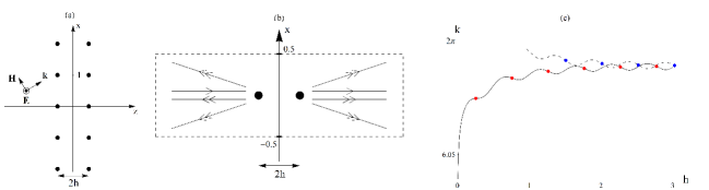
Figure 1: Panel (a): Double array of dielectric cylinders. The unit of length is the array period. The axis of each cylinder is parallel to the $y$-axis, and is at a distance $h$ from the $x$-axis.
Panel (b): The scattering process for the normal incident radiation (${k_{x}}=0$). The scattered fundamental harmonic is symbolized by a single headed arrow while the (generated) second harmonic radiation is symbolized by a double headed arrow. The incident radiation wave length is such that only one diffraction channel is open for the fundamental harmonic while three diffraction channels are open for the second harmonic. The flux measured through the faces $L_{\pm 1/2}:x=\pm 1/2$ cancels out due to the Bloch periodicity condition as explained in Appendix B.
Panel (c): The solid and dashed curves show the position (frequency $\omega_{r}=ck_{r}$) of scattering resonances as functions of the distance between the arrays, $k=k_{r}(h)$. The dots on the curves indicate positions of bound states in the radiation continuum (i.e., the values of $h$ at which a resonance turns into a bound state). The solid curve connects bound states symmetric relative to the reflection $z\rightarrow-z$. The dashed line connects the skew symmetric bound states. The curves are realized for $R=0.08,\,{\varepsilon_{c}}=2$, and ${k_{x}}=0$ (normal incidence).

The solution of the integral equation (12) is obtained for $k^{2}$ near $k_{b}^{2}$ in the limit of subwavelength dielectric cylinders. The approximation is defined by a small parameter

$${\delta_{0}}(q)=\frac{(qR)^{2}}{4}({\varepsilon_{c}}-1)\ll 1$$ (17)

which is the scattering phase of a plane wave with the wavenumber $q$ on a single cylinder of radius $R$. For sufficiently small $R$, this approximation is justified. The integral kernel of ${\widehat{\text{H}}}(q^{2})$ is defined by (7) and has support on the region occupied by cylinders. The condition (17) implies that the wavelength is much larger than the radius $R$, and therefore field variations within each cylinder may be neglected, so that $\psi(x,z)\approx\psi(n,\pm h)$ where $(n,\pm h)$ are the positions of the axes of the cylinders ($n$ is an integer). The integration in ${\widehat{\text{H}}}(q^{2})[\psi]$ yields then an infinite sum over positions of the cylinders. By Bloch’s condition, $\psi(n,\pm h)=e^{inq_{x}}\psi(0,\pm h)$, so that the function ${\widehat{\text{H}}}(q^{2})[\psi](x,z)$ is fully determined by the two values $\psi(0,\pm h)$. In particular,

$${\widehat{\text{H}}}(q^{2})[\psi](0,\pm h)\approx\alpha\psi(0,\pm h)+\beta\psi(0,\mp h)$$ (18)

where the coefficients $\alpha$ and $\beta$ are shown to be jmp

$$\alpha(q,q_{x})=2\pi i{\delta_{0}}(q)\left(\sum_{m=-\infty}^{\infty}\left(\frac{1}{q_{z,m}}-\frac{1}{2\pi i(|m|+1)}\right)+\frac{i}{\pi}\ln(2\pi R)\right)$$ (19)

$$\beta(q,q_{x},h)=2\pi i{\delta_{0}}(q)\sum_{m=-\infty}^{\infty}\frac{e^{2ihq_{z,m}}}{q_{z,m}}$$

where $q_{z,m}=\sqrt{q^{2}-(q_{x}+2\pi m)^{2}}$ with the convention that if $q^{2}<(q_{x}+2\pi m)^{2}$, then $q_{z,m}=i\sqrt{(q_{x}+2\pi m)^{2}-q^{2}}$. To obtain the energy flux scattered by the structure, the action of the operator ${\widehat{\text{H}}}(q^{2})$ on $\psi$ must be determined in the asymptotic region $|z|\rightarrow\infty$. It is found that for $|z|>h+R$,

$${\widehat{\text{H}}}(q^{2})[\psi](x,z)\approx 2\pi i{\delta_{0}}(q)\sum_{m=-\infty}^{\infty}\left(\psi(0,h)e^{i|z-h|q_{z,m}}+\psi(0,-h)e^{i|z+h|q_{z,m}}\right)\frac{e^{ix(q_{x}+2\pi m)}}{q_{z,m}}$$ (20)

IV Amplitudes of the fundamental and second harmonics

Now that the action of the operator ${\widehat{\text{H}}}(q^{2})$ has been established in (18) and (20), the amplitudes $E_{1}$ and $E_{2}$ of the fundamental and second harmonics can be determined by solving the system (10). As noted earlier, this will be done along a curve ${\mathscr{C}}$ in the $h,k$-plane defined by $k=k_{r}(h)$ where $k_{r}(h)$ is the real part of a pole of $[1-{\widehat{\text{H}}}(k^{2})]^{-1}$, or equivalently, when the incident radiation has the resonant wave number $k=k_{r}(h)$. To find the curve, the eigenvalue problem (11) is solved in in the approximation (18):

$$[1-{\mathscr{H}}]\begin{pmatrix}E_{b+}\\ E_{b-}\end{pmatrix}=\begin{pmatrix}0\\ 0\end{pmatrix},\quad{\mathscr{H}}=\begin{pmatrix}{\alpha}&{\beta}\\ {\beta}&{\alpha}\end{pmatrix}$$ (21)

where $E_{b\pm}=E_{b}(0,\pm h)$ and the functions ${\alpha}={\alpha}(k,{k_{x}})$ and ${\beta}={\beta}(k,{k_{x}})$ have been defined in the previous section. In particular, bound states occur at the points $({h_{b}},{k_{b}})$ at which the determinant $\det(1-{\mathscr{H}})$ vanishes,

$$\det\begin{pmatrix}1-{\alpha}&-{\beta}\\ -{\beta}&1-{\alpha}\end{pmatrix}=(1-{\alpha}-{\beta})(1-{\alpha}+{\beta})=0$$

It follows from Eq.(21) that the bound states for which $1-{\alpha}-{\beta}=0$ are even in $z$ because $E_{b+}=E_{b-}$ in this case. Similarly, the bound states for which $1-{\alpha}+{\beta}=0$ are odd in $z$. More generally, the poles of the resolvent $[1-{\widehat{\text{H}}}(k^{2})]^{-1}$ are complex zeros of $\det(1-{\mathscr{H}})$. They are found by the conventional scattering theory formalism. Specifically, the resonant wave numbers $k^{2}=k^{2}_{r}(h)$ are obtained by solving the equation ${\text{Re}}\{1-{\alpha}\pm{\beta}\}=0$ for the spectral parameter $k^{2}$. According to the convention adopted in the representation (14), the corresponding resonance widths are defined by

$$\Gamma(h)=-\frac{{\text{Im}}\{1-{\alpha}\pm{\beta}\}}{\partial_{k^{2}}{\text{Re}}\{1-{\alpha}\pm{\beta}\}}\bigg{|}_{k^{2}=k^{2}_{r}(h)}$$

where $\partial_{k^{2}}$ denotes the derivative with respect to $k^{2}$. This definition of the width corresponds to the linearization of ${\text{Re}}\{1-{\alpha}\pm{\beta}\}$ near $k^{2}=k^{2}_{r}(h)$ as a function of $k^{2}$ in the pole factor $[1-{\alpha}\pm{\beta}]^{-1}$. The curves of resonances $k=k_{r}(h)>{k_{x}}$ come in pairs. There is a curve connecting the symmetric bound states in the $h,k$-plane, and another curve that connects the odd ones.

In what follows, only the curve connecting symmetric bound states will be considered. The other curve can be treated similarly. Panel (c) of Fig. 1 shows that the first symmetric bound state occurs when the distance $2h$ is about half the array period, while the skew-symmetric bound states emerge only at larger distances. This feature is explained in detail in jmp . So, the solution obtained near the first symmetric bound state corresponds to the smallest possible transverse dimension of the system (roughly a half of the wave length of the incident radiation). Thus, from now on the curve of resonances ${\mathscr{C}}$ refers to the curve in the $h,k$-plane defined by the equation ${\text{Re}}\{1-{\alpha}-{\beta}\}=0$. To simplify the technicalities, it will be further assumed that only one diffraction channel is open for the fundamental harmonics, i.e., ${k_{x}}<k<2\pi-{k_{x}}$.

Let $k=k_{r}(h)$ be the solution of ${\text{Re}}\{1-{\alpha}-{\beta}\}=0$. By making use of the explicit form of the functions $\alpha$ and $\beta$ for one open diffraction channel, one infers that along the curve $k=k_{r}(h)$,

$$1-{\alpha}-{\beta}=i{\text{Im}}\{1-{\alpha}-{\beta}\}=-i\frac{4\pi{\delta_{0}}(k_{b})}{k_{z}}{\varphi}^{2},\,\quad{\varphi}=\cos(hk_{z}),\ \quad k_{z}=\sqrt{k^{2}_{b}-k_{x}^{2}}$$

Bound states in the radiation continuum occur when the distance $h$ satisfies the equation ${\varphi}=0$, i.e., $h\sqrt{k_{r}^{2}(h)-k_{x}^{2}}=(n-1/2)\pi$ with $n$ being a positive integer. Its solutions $h={h_{b}}(n)$ define the corresponding values of the wave numbers of the bound states, $k_{b}(n)=k_{r}({h_{b}}(n))$. So, the sequence of pairs $\{({h_{b}}(n),{k_{b}}(n))\}_{n=1}^{\infty}$ indicates positions of the bound states on the curve ${\mathscr{C}}$. In the limit $h\rightarrow{h_{b}}(n)$ along ${\mathscr{C}}$, the function ${\varphi}$ has the asymptotic behavior,

$${\varphi}=(-1)^{n}k_{z,b}\Delta h+o(\Delta h),\quad k_{z,b}={k_{z}}|_{h=h_{b}(n)},\quad\Delta h=h-{h_{b}}$$

The objective is to determine the dependence of the amplitudes $E_{1}$ and $E_{2}$ on the parameters $\Delta h$ and ${\chi_{c}}$ which are both small.

To this end, let $E_{1\pm}=E_{1}(0,\pm h)$ be the values of the field $E_{1}$ on the axes of the cylinders at $(0,\pm h)$, and $E_{2\pm}=E_{2}(0,\pm h)$ be the values of the field $E_{2}$ on the same cylinders. In the subwavelength approximation, these values determine the scattered field because the latter is produced by the radiation of point dipoles induced by the incident wave on the scatterers and the strength of the dipoles is proportional to $E_{1\pm}$ for the fundamental harmonic and $E_{2\pm}$ for the second harmonic. Applying the rule (18) to evaluate the action of the operator ${\widehat{\text{H}}}(q^{2})$ in the system (10), the first equation of the latter becomes,

$$[1-{\mathscr{H}}]\begin{pmatrix}E_{1+}\\ E_{1-}\end{pmatrix}=2\nu{\mathscr{H}}\begin{pmatrix}\overline{E}_{1+}E_{2+}\\ \overline{E}_{1-}E_{2-}\end{pmatrix}+\begin{pmatrix}e^{+ih{k_{z}}}\\ e^{-ih{k_{z}}}\end{pmatrix}$$ (22a)

Similarly, the second of Eqs.(10) yields,

$$[1-{\mathscr{H}_{2}}]\begin{pmatrix}E_{2+}\\ E_{2-}\end{pmatrix}=\nu{\mathscr{H}_{2}}\begin{pmatrix}E_{1+}^{2}\\ E_{1-}^{2}\end{pmatrix},\quad{\mathscr{H}_{2}}={\mathscr{H}}(2k,2{k_{x}})$$ (22b)

As stated above, the resolvent $[1-{\widehat{\text{H}}}((2k)^{2})]^{-1}$ is regular in a neighborhood of ${k_{b}}$ so that Eq. (22b) can be solved for $E_{2\pm}$, which defines the latter as functions of $E_{1\pm}$. The substitution of this solution into Eq.(22a) gives a system of two nonlinear equations for the fields $E_{1\pm}$. Adding these equations and replacing the field $E_{1-}$ by its expression $E_{1-}=\mu(0,h)E_{1+}$ in terms of the field ratio of Eq.(13) yields the following implicit relation between the field $E_{1+}$ and its amplitude $|E_{1+}|$:

$$E_{1+}=-\frac{{\varphi}}{\frac{\nu^{2}}{\zeta}|E_{1+}|^{2}+{\varphi}^{2}\xi}$$ (23)

where ${\varphi}=\cos(h{k_{z}})$ and $\nu=\frac{{\chi_{c}}}{4\pi({\varepsilon_{c}}-1)}$ are small and, in terms of the field ratio $\mu\equiv\mu(0,h)$, the values of $\zeta$ and $\xi$ read,

$$\xi=i\frac{2\pi{\delta_{0}}(k)}{{k_{z}}}(1+\mu),\quad\frac{1}{\zeta}=\left(1+i\frac{4\pi{\delta_{0}}(k)}{{k_{z}}}{\varphi}^{2}\right)\left(a+b\mu^{2}+\overline{\mu}\left(b+a\mu^{2}\right)\right)$$ (24)

with $a$ and $b$ being defined by the relation,

$$[1-{\mathscr{H}_{2}}]^{-1}{\mathscr{H}_{2}}=\begin{pmatrix}a&b\\ b&a\end{pmatrix}$$ (25)

In particular, $\zeta$ and $\xi$ are continuous functions of $\mu$ and ${\varphi}$. In Appendix A it is shown that if $\zeta_{b}$ and $\xi_{b}$ are the respective limits of $\zeta$ and $\xi$ as $h\rightarrow{h_{b}}$ along the curve of resonances ${\mathscr{C}}$, then these limits are nonzero. It follows then that Eq.(23) for $E_{1+}$ is singular in both $\nu$ and ${\varphi}$ when these parameters are small, i.e., in the limit $(\nu,{\varphi})\rightarrow(0,0)$. Furthermore, there is no way to solve the said equation perturbatively in either of the parameters. A full non-perturbative solution can be obtained using Cardano’s method for solving cubic polynomials. Indeed, by taking the modulus squared of both sides of the equation, it is found that,

$$X^{3}+2\frac{{\varphi}^{2}}{\nu^{2}}{\text{Re}}\{\zeta\xi\}X^{2}+\frac{{\varphi}^{4}}{\nu^{4}}|\zeta\xi|^{2}X-\frac{{\varphi}^{2}}{\nu^{4}}|\zeta|^{2}=0,\quad X=|E_{1+}|^{2}$$ (26)

The solution to this cubic equation is obtained in Appendix C. It is proved there that Eq. (26) admits a unique real solution so that there is no ambiguity on the choice of $E_{1+}$. In the vicinity of a point $({h_{b}},{k_{b}})$ along the resonance curve ${\mathscr{C}}$, the field $E_{1+}$ is found to behave as,

$$|E_{1+}|=\frac{|\Delta h|^{1/3}}{{\chi_{c}}}\,\tau(\Delta h,{\chi_{c}})$$ (27)

Recall that $\Delta h=h-{h_{b}}$. An explicit form of the function $\tau(\Delta h,{\chi_{c}})$ is given in Appendix C (see Eq. (40)). It involves combinations of the square and cube roots of functions in $\Delta h$ and ${\chi_{c}}$ and has the property that $\tau(\Delta h,{\chi_{c}})\rightarrow 0$ as $(\Delta h,{\chi_{c}})\rightarrow(0,0)$ (in the sense of the two-dimensional limit). In the limit $h\rightarrow h_{b}$, the field ratio $\mu$ approaches $1$ for a symmetric bound state as argued earlier. Therefore it follows from Eqs.(22b) that $E_{2\pm}\sim\nu E_{1+}^{2}$ because the matrix (25) exists at $h=h_{b}$. Since $\nu\sim\chi_{c}$, relation (27) leads to the conclusion that

$$\frac{E_{2\pm}}{E_{1+}}=O(|\Delta h|^{1/3})$$

Thus, the approximation $|E_{1}|\gg|E_{2}|$ used to truncate the system (10) remains valid for $h$ close to the critical value ${h_{b}}$ despite the non-analyticity of the amplitudes at $(\Delta h,\chi_{c})=(0,0)$.

V Flux analysis: the conversion efficiency

For the nonlinear system considered, even though Poynting’s theorem takes a slightly different form as compared to linear Maxwell’s equations, the flux conservation for the time averaged Poynting vector holds. The scattered energy flux carried across a closed surface by each of the different harmonics adds up to the incident flux across that surface. The flux conservation theorem is stated in Appendix B. Consider a closed surface that consists of four faces, $L_{\pm}=\{(x,z)|-\frac{1}{2}\leq x\leq\frac{1}{2},z\rightarrow\pm\infty\}$ and $L_{\pm 1/2}=\{(x,z)|x=\pm 1/2\}$ as depicted in Fig. 1(b). As argued in Appendix B, the scattered flux of each $l^{\text{th}}$-harmonics across the union of the faces $L_{\pm 1/2}$ vanishes because of the Bloch condition (and so does the incident flux for any $k_{x}$). Therefore only the flux conservation across the union of the faces $L_{\pm}$ has to be analyzed. If $\sigma_{l}$ designates the ratio of the scattered flux carried by the $l^{\text{th}}$-harmonics across the faces $L_{\pm}$ to the incident flux across the same faces, then $\sum_{l\geq 1}\sigma_{l}=1$. Thus, for $l\geq 2$, $\sigma_{l}$ defines the conversion ratio of fundamental harmonics into the $l^{\text{th}}$-harmonics.

In the perturbation theory used here, only the ratios $\sigma_{1}$ and $\sigma_{2}$ may be evaluated. By laborious calculations it can be shown that $\sigma_{1}+\sigma_{2}\leq 1$ as one would expect (see Appendix B for details). Hence, the efficiency of converting the fundamental harmonic into the second harmonic is simply determined by the maximum value of $\sigma_{2}$ as a function of the parameter $h$ at a given value of the nonlinear susceptibility $\chi_{c}$.

The ratio $\sigma_{2}$ is defined in terms of the scattering amplitudes of the second harmonic, i.e., by the amplitude of $E_{2}$ in the asymptotic region $|z|\rightarrow\infty$:

$$E_{2}({\mathbf{r}})\rightarrow\begin{cases}\displaystyle{\sum_{m^{op,sh}}R_{m}^{sh}e^{i{\mathbf{r}}\cdot\mathbf{k}_{m,sh}^{-}}},\quad z\rightarrow-\infty\\ \displaystyle{\sum_{m^{op,sh}}T_{m}^{sh}e^{i{\mathbf{r}}\cdot\mathbf{k}_{m,sh}^{+}}},\quad z\rightarrow+\infty\end{cases}$$ (28)

where $\mathbf{k}_{m,sh}^{\pm}=(2k_{x}+2\pi m){\mathbf{e}_{1}}\pm k_{z,m}^{sh}{\mathbf{e}_{3}}$ is the wave vector of the second harmonic in the $m^{\text{th}}$ open diffraction channel. Recall that the $m^{\text{th}}$ channel is open provided $(2k)^{2}>(2{k_{x}}+2\pi m)^{2}$ and in this case $k_{z,m}^{sh}=\sqrt{(2k)^{2}-(2{k_{x}}+2\pi m)^{2}}$, while if the channel is closed, then $k_{z,m}^{sh}=i\sqrt{(2{k_{x}}+2\pi m)^{2}-(2k)^{2}}$. In the asymptotic region $|z|\rightarrow\infty$, the field in closed channels decays exponentially and, hence, the energy flux can only be carried in open channels to the spatial infinity. The summation in Eqs.(28) is taken only over those values of $m$ for which the corresponding diffraction channel is open for the second harmonic, which is indicated by the superscript “$op,sh$” in the summation index $m^{op,sh}$. Note that there is more than one open diffraction channel for the second harmonic even though only one diffraction channel is open for the fundamental one. For instance, if the $x-$component of the wave vector ${\mathbf{k}}$, i.e., ${k_{x}}$, is less than $\frac{\pi}{2}$, there are 3 open diffraction channels for the second harmonic, the channels $m=0,\,m=-1$, and $m=1$. These three directions of the wave vector of the second harmonic propagating in each of the asymptotic regions $z\rightarrow\pm\infty$ are depicted in Fig. 1(b) by double-arrow rays. Thus, in terms of the scattering amplitudes introduced in Eqs. (28), the ratio of the second harmonic flux across $L_{\pm}$ to the incident flux is

$$\sigma_{2}=\frac{1}{2{k_{z}}}\sum_{m^{op,sh}}k_{z,m}^{sh}\left(|R_{m}^{sh}|^{2}+|T_{m}^{sh}|^{2}\right)$$

The scattering amplitudes $R_{m}^{sh}$ and $T_{m}^{sh}$ are inferred from Eq.(9) in which the rule (20) is applied to calculate the action of the operator ${\widehat{\text{H}}}((2k)^{2})$ in the far-field regions $|z|\rightarrow\infty$:

$$\begin{cases}\displaystyle{R_{m}^{sh}=\frac{2\pi i{\delta_{0}}(2k)}{k_{z,m}^{sh}}\left[(E_{2+}+\nu E_{1+}^{2})e^{ihk_{z,m}^{sh}}+(E_{2-}+\nu E_{1-}^{2})e^{-ihk_{z,m}^{sh}}\right]}\vspace{0.1 cm}\\ \displaystyle{T_{m}^{sh}=\frac{2\pi i{\delta_{0}}(2k)}{k_{z,m}^{sh}}\left[(E_{2+}+\nu E_{1+}^{2})e^{-ihk_{z,m}^{sh}}+(E_{2-}+\nu E_{1-}^{2})e^{ihk_{z,m}^{sh}}\right]}\end{cases}$$

Since for $\nu\neq 0$, the amplitudes $E_{1\pm}$ remain finite as $h\rightarrow{h_{b}}$ along ${\mathscr{C}}$, and since $\mu\rightarrow 1$ in the said limit; the principal part of $\sigma_{2}$ in a vicinity of a bound state along the curve ${\mathscr{C}}$ is obtained by setting $E_{1-}=E_{1+}$ in Eq. (22b), solving the latter for $E_{2\pm}$, and substituting the solution into the expression for $\sigma_{2}$. The result reads

$$\sigma_{2}=C_{b}\nu^{2}|E_{1+}|^{4}$$ (29)

where $C_{b}$ is a constant obtained by taking all nonsingular factors in the expression of $\sigma_{2}$ to their limit as $h\rightarrow{h_{b}}$, which gives

$$C_{b}=\left[\frac{(16\pi{\delta_{0}}(k))^{2}}{{k_{z}}}\left|1+a+b\right|^{2}\sum_{m^{op,sh}}\frac{\cos^{2}(hk_{z,m}^{sh})}{k_{z,m}^{sh}}\right]_{(h,k)=({h_{b}},{k_{b}})}$$

for $a$ and $b$ defined in Eq.(25). Using the identity $|E_{1+}|^{4}=|E_{1+}|^{2}|E_{1+}|^{2}$, and substituting Eq.(23) into one of the factors $|E_{1+}|^{2}$, the conversion ratio $\sigma_{2}$ is expressed as a function of a single real variable,

$$\sigma_{2}(u)=C_{b}^{\prime}\frac{u}{|u+\zeta_{b}\xi_{b}|^{2}},\,\quad u=\left(\frac{\nu|E_{1+}|}{{\varphi}}\right)^{2}$$ (30)

where $C_{b}^{\prime}=C_{b}|\zeta_{b}|^{2}$ is a constant, and $\xi$ and $\zeta$ in Eq.(24) have been taken at their limits as $h\rightarrow{h_{b}}$ to obtain the principal part of $\sigma_{2}$. The function $u\mapsto\sigma_{2}(u)$ on $[0,\infty)$ is found to attain its absolute maximum at $u=|\xi_{b}\zeta_{b}|$. This condition determines the distance $2h$ between the arrays at which the conversion rate is maximal for given parameters $R,\,{\varepsilon_{c}}$ and ${\chi_{c}}$ of the system. Indeed, since $u\sim|E_{1+}|^{2}$ should also satisfy the cubic equation (26), the substitution of $u=|\zeta_{b}\xi_{b}|$ into the latter yields the condition

$$\frac{\nu^{2}}{{\varphi}^{4}}=2|\xi_{b}|^{2}\left(|\xi_{b}\zeta_{b}|+{\text{Re}}\{\xi_{b}\zeta_{b}\}\right)$$ (31a)

In particular, in the leading order in $${\delta_{0}}(k) 2h$$, the optimal distance between the two arrays is given by the formula,

$$(h-{h_{b}})^{4}=\frac{\chi_{c}^{2}}{8\pi^{5}k_{z,b}({k_{b}}R)^{6}({\varepsilon_{c}}-1)^{5}}$$ (31b)

where as previously, $k_{z,b}=\sqrt{k_{b}^{2}-k_{x}^{2}}$.

The maximum value $\sigma_{2,{\rm max}}$ of the conversion ratio $\sigma_{2}$ is the sought-for conversion efficiency. An interesting feature to note is that $\sigma_{2,{\rm max}}=\sigma_{2}(|\zeta_{b}\xi_{b}|)$ is independent of the nonlinear susceptibility $\chi_{c}$ because the constants $C_{b}^{\prime}$, $\xi_{b}$, and $\zeta_{b}$ are fully determined by the position of the bound state $(k_{b},h_{b})$. In other words, if the distance between the arrays is chosen to satisfy the condition (31a), the conversion efficiency $\sigma_{2,{\rm max}}$ is the same for a wide range of values of the nonlinear susceptibility $\chi_{c}$. This conclusion follows from two assumptions made in the analysis. First, the subwavelength approximation should be valid for both the fundamental and second harmonics, i.e., the radius of cylinders should be small enough. Second, the values of $h-h_{b}$ and $\nu$ (or $\chi_{c}$) must be such that the analysis of the existence and uniqueness of $|E_{1+}|$ given in Appendix C holds, that is, Eq. (26) should have a unique real solution under the condition (31a). The geometrical and physical parameters of the studied system can always be chosen to justify these two assumptions as illustrated in Fig. 2.

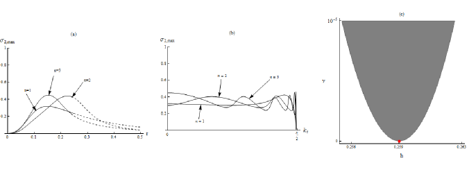
Figure 2: Panel (a): The conversion efficiency is plotted against the cylinder radius $R$ for the critical points $({h_{b}}(n),{k_{b}}(n)),\,n=1,2,3$, and ${\varepsilon_{c}}=1.5$ and ${k_{x}}=0$ (the normal incidence). The dashed parts of the curves indicate the regions where ${\delta_{0}}(k)>0.25$ and, hence, ${\delta_{0}}(2k)>1$, i.e., the subwavelength approximation becomes inapplicable for the second harmonic.
Panel (b): The conversion efficiency is plotted against ${k_{x}}$ for the critical points $({h_{b}}(n),{k_{b}}(n)),\,n=1,2,3$. The curves are realized for $R=0.15$ and ${\varepsilon_{c}}=1.5$.
Panel (c): The region of validity of the developed theory for the first bound state ${h_{b}}(1)\approx 0.259$. The shadowed part of the $(\nu,h)-$plane is defined by the condition $\tau_{+}+\tau_{-}>0$ under which, according to Eq.(40), the amplitude $|E_{1+}|$ exists and unique as explained in Appendix C. The plot is realized for $R=0.1,\,{\varepsilon_{c}}=2$ and ${k_{x}}=0$. The parabola-like curve is an actual boundary of the shadowed region; the top horizontal line represents no restriction. So there is a wide range of the physical and geometrical parameters within the shadowed region which satisfy (31a). The regions of validity for other bound states looks similar.

Panels (a) and (b) of Fig. 2 show the conversion efficiency $\sigma_{2,{\rm max}}$ for the first three symmetric bound states $n=1,2,3$, as, respectively, a function of the cylinder radius $R$ when $k_{x}=0$ and of $k_{x}$ when $R=0.15$. For all curves presented in the panels, $\varepsilon_{c}=1.5$. The values of $\sigma_{2,{\rm max}}$ are evaluated numerically by Eq. (30) where $u=|\xi_{b}\zeta_{b}|$. The solid parts of the curves in Panel (a) correspond to the scattering phase $\delta_{0}(k)<0.25$ with $k=k_{b}$. Note that the wavelength at which the second harmonic generation is most efficient is the resonant wavelength defined by $k=k_{r}(h)$ where $h$ satisfies the condition (31a). For a small $\chi_{c}$, the scattering phase at the resonant wavelength can well be approximated as $\delta_{0}(k)\approx\delta_{0}(k_{b})$. The condition $\delta_{0}(k_{b})<0.25$ ensures that the scattering phase for the second harmonic satisfies the inequality $\delta_{0}(2k_{b})=4\delta_{0}(k_{b})<1$ otherwise the validity of the subwavelength approximation cannot be justified. The dashed parts of the curves in Panels (a) of Fig. 2 correspond to the region where $\delta_{0}(k_{b})>0.25$. Panels (a) and (b) of the figure show that the conversion efficiency can be as high as 40% for a wide range of the incident angles and values of the cylinder radius. Such a conversion efficiency is comparable with that achieved in optically nonlinear crystals at a typical beam propagation length (active length) of a few centimeters, whereas here the transverse dimension $2h$ of the system studied here can be as low as a half of the wavelength, i.e., for an infrared incident radiation, $2h$ is about a few hundred nanometers. Indeed, as one can see in Fig. 1(c), the first bound state occurs at $h_{b}(1)\approx 0.259$ and $k_{b}\approx 2\pi$ which corresponds to the wavelength $\lambda_{b}=2\pi/k_{b}\approx 1$.

The stated conversion efficiency can be fairly well estimated in the leading order of ${\delta_{0}}(k)$:

$$\sigma_{2,{\rm max}}=\sigma_{2}(|\zeta_{b}\xi_{b}|)\approx 8\pi{\delta_{0}}(k)\sum_{m^{op,sh}}\frac{\cos^{2}(hk_{z,m}^{sh})}{k_{z,m}^{sh}}\Bigg{|}_{(h,k)=({h_{b}},{k_{b}})}$$ (32)

Suppose that only one diffraction channel is open for the incident radiation. Then $m=0,\pm 1$ in Eq.(32) (three open channels for the second harmonics). Let $\sigma_{2,{\rm max}}^{0}$ denote the term $m=0$, i.e. $\sigma_{2,{\rm max}}^{0}$ is the second harmonic flux in which the contribution of the channels with $m=\pm 1$ is omitted. In particular, $\sigma_{2,{\rm max}}^{0}<\sigma_{2,{\rm max}}$. One infers from Eq. (32) that,

$$\sigma_{2,{\rm max}}^{0}\approx\frac{4\pi{\delta_{0}}({k_{b}})}{k_{z,b}}\cos^{2}(2{h_{b}}k_{z,b})$$

As the pair $({h_{b}},{k_{b}})$ at which a symmetric bound state is formed satisfies the equation $\cos({h_{b}}k_{z,b})=0$, it follows that $\cos(2{h_{b}}k_{z,b})=-1$. Hence,

$$\sigma_{2,{\rm max}}^{0}\approx\frac{k_{b}^{2}}{k_{z,b}}\pi R^{2}({\varepsilon_{c}}-1)$$

The wavenumbers ${k_{b}}$ at which the bound states occur lie just below the diffraction threshold $2\pi-{k_{x}}$, i.e., ${k_{b}}\lessapprox 2\pi-{k_{x}}$ (see Fig. 1(c) and jmp for details). So that in the case of normal incidence (${k_{x}}=0$), the above estimate becomes,

$$\sigma_{2,{\rm max}}^{0}\approx 2\pi(\pi R^{2})({\varepsilon_{c}}-1)$$

with $\delta_{0}(2\pi)\ll 1$. If, for instance, $R=0.15$ and ${\varepsilon_{c}}=2$, then,

$$\sigma_{2,{\rm max}}^{0}\approx 44\%$$

for $\delta_{0}(2\pi)\approx 0.22$.

Appendices

Appendix A Estimation of $\zeta$ and $\xi$

Here the limit values $\zeta_{b}$ and $\xi_{b}$ of the functions $\zeta$ and $\xi$ defined in Eq. (24) are estimated as $h\rightarrow h_{b}$ along the resonance curve ${\mathscr{C}}$. For $\xi_{b}$ this is immediate. Indeed, in the aforementioned limit, the field ratio $\mu\rightarrow 1$ for a symmetric bound state and, therefore,

$$\xi_{b}=i\frac{4\pi{\delta_{0}}(k)}{{k_{z}}}\Bigg{|}_{k={k_{b}}}$$

For $\zeta_{b}$, the estimate follows from that wave numbers ${k_{b}}$ at which bound states exist are close to the diffraction threshold $2\pi-{k_{x}}$ when only one diffraction channel is open for the fundamental harmonic, i.e., ${k_{x}}<k<2\pi-{k_{x}}$ jmp . Indeed, in the first order of ${\delta_{0}}(k)$,

$$k_{b}\approx 2\pi-{k_{x}}-\frac{8\pi^{2}\delta_{0}^{2}(2\pi-{k_{x}})}{2\pi-{k_{x}}}$$ (33)

This proximity of the wavenumbers ${k_{b}}$ to the diffraction threshold $2\pi-{k_{x}}$ allows one to determine the leading terms in the coefficients $a$ and $b$ defined in Eq.(25), and hence $\zeta_{b}$. To proceed, the coefficients ${\alpha_{2}}=\alpha(2k,2{k_{x}})$ and ${\beta_{2}}=\beta(2k,2{k_{x}},h)$ of the matrix ${\mathscr{H}_{2}}$ are rewritten by separating explicitly the real and imaginary parts:

$${\alpha_{2}}+{\beta_{2}}=\psi_{+}+iS_{c},\quad{\alpha_{2}}-{\beta_{2}}=\psi_{-}+iS_{s}$$ (34a)

where $$S_{c} S_{s}$$ and are defined by the relations,

$$S_{c}=16\pi{\delta_{0}}(k)\sum_{m^{op,sh}}\frac{\cos^{2}(hk_{z,m}^{sh})}{k_{z,m}^{sh}},\quad S_{s}=16\pi{\delta_{0}}(k)\sum_{m^{op,sh}}\frac{\sin^{2}(hk_{z,m}^{sh})}{k_{z,m}^{sh}}$$ (34b)

and the index $m^{op,sh}$ indicates that the summations are to be taken over all open diffraction channels for the second harmonic. Using the estimate (33), the functions $\psi_{\pm}$ are found to obey the estimates,

$$\psi_{+}=2+O(\delta_{0}({k_{b}})),\quad\,\psi_{-}=O(\delta_{0}({k_{b}}))$$

These expressions are then used to estimate $\zeta_{b}^{-1}=2(a+b)$. In the first order of $\delta_{0}({k_{b}})$ one infers that

$$\zeta_{b}\approx-\frac{1}{4}-2\pi i{\delta_{0}}(k)\sum_{m^{op,sh}}\frac{\cos^{2}(hk_{z,m}^{sh})}{k_{z,m}^{sh}}\Bigg{|}_{(h,k)=({h_{b}},{k_{b}})}$$ (35)

Appendix B Complements on the flux analysis: Flux conservation

For the nonlinear wave equation (2), the Poynting Theorem becomes,

$$\frac{1}{8\pi}\frac{d}{dt}\left[\int_{V}\left({\varepsilon}E^{2}+B^{2}+\frac{\chi}{3\pi}E^{3}\right)d{\bf r}\right]=-\int_{\partial V}\mathbf{S}\cdot d\mathbf{n}$$ (36)

where $V$ is a closed region, and $\partial V$ is its boundary. The vector $\mathbf{S}=\mathbf{E}\times\mathbf{B}$ is the Poynting vector (for simplicity, it is assumed that $\partial V$ lies in the vacuum so that $\mu=\varepsilon=1$, and $\chi=0$ in a small neighborhood of $\partial V$). In the case of a monochromatic incident wave, the flux measured is the time-average of ${\bf S}$ over a time interval $T\rightarrow\infty$. By averaging Eq.(36), it then follows that,

$$\int_{\partial V}\langle\mathbf{S}\rangle\cdot d\mathbf{n}=\mathbf{0},\quad\,\langle\mathbf{S}\rangle=\frac{1}{T}\int_{0}^{T}\mathbf{S}(t)dt,\quad T\rightarrow\infty$$

This is the flux conservation. In terms of the different harmonics of Eq.(4), the time averaged Poynting vector becomes,

$$\langle\mathbf{S}\rangle=-\frac{c^{2}}{2\pi\omega}{\text{Im}}\left(\sum_{l=1}^{\infty}\frac{E_{l}\nabla E_{-l}}{l}\right)$$

Of interest is the flux of the Poynting vector across the rectangle depicted in Fig. 1(b). By Bloch’s condition (5), the contributions to the flux from the faces $L_{\pm 1/2}:x=\pm\frac{1}{2}$ cancel out so that the flux measured is through the vertical faces $L_{\pm}=\{(x,z)|-\frac{1}{2}\leq x\leq\frac{1}{2},\,z\rightarrow\pm\infty\}$. Note that the vanishing of the flux across the faces $L_{\pm 1/2}$ is a consequence of the fact that the incident wave is uniformly extended over the whole $x-$axis. For example, consider the normal incidence ($k_{x}=0$) with one diffraction channel open for the incident radiation. Then the Poynting vector of the reflected and transmitted fundamental harmonic is normal to the structure and, hence, carries no flux across $L_{\pm 1/2}$. The second harmonic $(l=2)$ has three forward and three backward scattering channels open, $m=0,\pm 1$, relative to the $z-$axis. The wave with $m=0$ propagates in the direction normal to the structure and does not contribute to the flux across $L_{\pm 1/2}$. Since the incident wave has an infinite front along the $x-$axis, so do the scattered waves with $m=\pm 1$. The waves with $m=1$ and $m=-1$ carry opposite fluxes across each of the faces $L_{\pm 1/2}$ as the corresponding wave vectors have the same $z-$components and opposite $x-$components and, hence, the total flux vanishes. For a finite wave front (but much larger than the structure period), the second harmonic would carry the energy flux in all the directions parallel to the corresponding wave vectors in each open diffraction channel.

If $\sigma_{l}$ is as defined in Section V, then the flux conservation implies that $\sum_{l=1}^{\infty}\sigma_{l}=1$. Therefore, in the perturbation theory used, i.e., when the system (6) is truncated to Eqs.(10), the inequality $\sigma_{1}+\sigma_{2}\leq 1$ must be verified to justify the validity of the theory.

The conversion ratio $\sigma_{2}$ is given in Section V. If only one diffraction channel is open for the fundamental harmonic, then the ratio $\sigma_{1}$ of the scattered and incident fluxes of the fundamental harmonic reads,

$$\sigma_{1}=|1+T_{0}|^{2}+|R_{0}|^{2}$$

where $T_{0}$ and $R_{0}$ are the transmission and reflection coefficients which are obtained from the far-field amplitude of $E_{1}$ as,

$$E_{1}\rightarrow\begin{cases}\displaystyle{e^{i{\mathbf{r}}\cdot{\mathbf{k}}}+R_{0}e^{i{\mathbf{r}}\cdot{\mathbf{k}}^{-}},\quad\,z\rightarrow-\infty}\\ \displaystyle{(1+T_{0})e^{i{\mathbf{r}}\cdot{\mathbf{k}}},\quad\quad\ \ z\rightarrow+\infty}\end{cases}$$

where ${\mathbf{k}}={k_{x}}{\mathbf{e}_{1}}+{k_{z}}{\mathbf{e}_{3}}$ is the incident wave vector and ${\mathbf{k}}^{-}={k_{x}}{\mathbf{e}_{1}}-{k_{z}}{\mathbf{e}_{3}}$ is the wave vector of the reflected fundamental harmonic. It then follows from Eqs.(8) and (20) that

$$\begin{cases}\displaystyle{R_{0}=i\frac{2\pi{\delta_{0}}(k)}{{k_{z}}}\Bigl{[}(E_{1+}+2\nu E_{2+}\overline{E}_{1+})e^{ih{k_{z}}}+(E_{1-}+2\nu E_{2-}\overline{E}_{1-})e^{-ih{k_{z}}}\Bigr{]}}\\ \displaystyle{T_{0}=i\frac{2\pi{\delta_{0}}(k)}{{k_{z}}}\Bigl{[}(E_{1+}+2\nu E_{2+}\overline{E}_{1+})e^{-ih{k_{z}}}+(E_{1-}+2\nu E_{2-}\overline{E}_{1-})e^{ih{k_{z}}}\Bigr{]}}\end{cases}$$

In the vicinity of a critical point $({h_{b}},{k_{b}})$, the coefficients $R_{0}$ and $T_{0}$ obey the estimate,

$$R_{0}\approx T_{0}\approx i\frac{4\pi{\delta_{0}}({k_{b}})}{k_{z,b}}{\varphi}E_{1+}\left(1+\frac{\nu^{2}|E_{1+}|^{2}}{\zeta_{b}}\right)$$

After some algebraic manipulations, it is found that,

$$\sigma_{1}+\sigma_{2}=1+\frac{8\pi{\delta_{0}}({k_{b}})}{k_{z,b}}\nu^{2}|E_{1+}|^{4}\left[A_{b}+\frac{4\pi{\delta_{0}}({k_{b}})}{k_{z,b}}{\varphi}^{2}\left({\text{Re}}\left\{\frac{1}{\zeta_{b}}\right\}+\frac{\nu^{2}|E_{1+}|^{2}}{|\zeta_{b}|^{2}}\right)\right]$$

where $A_{b}$ is the constant defined as,

$$A_{b}=\left[2S_{c}|a+b+1|^{2}-{\text{Im}}\left\{\frac{1}{\zeta}\right\}\right]_{(h,k)=({h_{b}},{k_{b}})}$$

and $S_{c}={\text{Im}}\{{\alpha_{2}}+{\beta_{2}}\}$ is introduced in Eqs.(34). Expressing $a$ and $b$ defined by (25) via the coefficients ${\alpha_{2}}$ and ${\beta_{2}}$ of the symmetric matrix ${\mathscr{H}_{2}}$, one also obtains

$$S_{c}={\text{Im}}\left\{\frac{a+b}{1+a+b}\right\}$$

Since at the point $({h_{b}},{k_{b}})$ the value of $\zeta$ is $\zeta_{b}=(2(a+b))^{-1}|_{(h,k)=({h_{b}},{k_{b}})}$, it follows that,

$$A_{b}=\left[2{\text{Im}}\left\{\frac{a+b}{1+a+b}\right\}|a+b+1|^{2}-2{\text{Im}}\{a+b\}\right]\Bigg{|}_{(h,k)=({h_{b}},{k_{b}})}$$

For general complex numbers $a$ and $b$, the expression in square brackets is always zero. Therefore $A_{b}=0$, and,

$$\sigma_{1}+\sigma_{2}=1+2\left(\frac{4\pi{\delta_{0}}({k_{b}})}{k_{z,b}}{\varphi}\nu|E_{1+}|^{2}\right)^{2}\left({\text{Re}}\left\{\frac{1}{\zeta_{b}}\right\}+\frac{\nu^{2}|E_{1+}|^{2}}{|\zeta_{b}|^{2}}\right)$$ (37)

By Eq. (35), ${\text{Re}}\{\zeta_{b}^{-1}\}\approx-4$. In Appendix C it is proved that $\nu^{2}|E_{1+}|^{2}=O({\varphi}^{2/3})$. Consequently, near the critical point $({h_{b}},{k_{b}})$, the right hand summand in Eq.(37) is negative so that $\sigma_{1}+\sigma_{2}\leq 1$ as required.

Appendix C Complements on the amplitude $E_{1}$

The amplitude of the field $E_{1+}$ is a root of the cubic polynomial in Eq.(26) which can be solved by Cardano’s method. Put $Y=X+\frac{2}{3}\left(\frac{{\varphi}}{\nu}\right)^{2}{\text{Re}}\{\zeta\xi\}$. For the new variable $Y$, Eq. (26) assumes the standard form,

$$Y^{3}+pY+q=0$$ (38)

where,

$$p=\frac{{\varphi}^{4}}{3\nu^{4}}\left(|\zeta\xi|^{2}-2{\text{Re}}\{(\zeta\xi)^{2}\}\right),\quad\,q=\frac{2{\varphi}^{6}}{27\nu^{6}}{\text{Re}}\{\zeta\xi\}\left(4{\text{Re}}\{(\zeta\xi)^{2}\}-5|\zeta\xi|^{2}\right)-\frac{{\varphi}^{2}}{\nu^{4}}|\zeta|^{4}$$

As the amplitude $E_{1}$ is uniquely defined by the system (6), it is therefore expected that the cubic in Eq.(38) should have a unique real solution in order for the theory to be consistent. The latter holds if and only if the discriminant

$$D_{3}=\frac{4}{27}p^{3}+q^{2}$$

is nonnegative. To prove that $D_{3}\geq 0$, note first that $|\zeta\xi|^{2}-2{\text{Re}}\{\zeta^{2}\xi^{2}\}>0$ in the vicinity of a critical point $({h_{b}},{k_{b}})$. This follows from the estimates established in Appendix A. Indeed, in the first order of $\delta_{0}({k_{b}})$,

$$|\zeta_{b}\xi_{b}|^{2}-2{\text{Re}}\{(\zeta_{b}\xi_{b})^{2}\}\approx\frac{3\pi^{2}}{k_{z}^{2}}\delta_{0}^{2}(k)\Bigg{|}_{k={k_{b}}}>0$$ (39)

Next, consider the complex number

$$\rho=\frac{4}{27}\left[2{\text{Re}}\{\zeta\xi\}\left(2{\text{Re}}\{(\zeta\xi)^{2}\}-\frac{5}{2}|\zeta\xi|^{2}\right)+i(|\zeta\xi|^{2}-2{\text{Re}}\{(\zeta\xi)^{2}\})^{\frac{3}{2}}\right]$$

The positivity condition (39) ensures that the coefficient of the complex number $i$ in the expression of $\rho$ is indeed real. After some algebraic manipulations, it can be shown that,

$$D_{3}=\frac{{\varphi}^{4}}{\nu^{12}}\Big{|}|\zeta|^{2}\nu^{2}-{\varphi}^{4}\rho\Big{|}^{2}$$

Thus $D_{3}\geq 0$ as required. The only real solution $Y$ to Eq.(38) is then,

$$Y=\sqrt[3]{\frac{-q+\sqrt{D_{3}}}{2}}+\sqrt[3]{\frac{-q-\sqrt{D_{3}}}{2}}$$

It then follows that,

$$|E_{1+}|=\frac{|{\varphi}|^{\frac{1}{3}}}{\nu}\sqrt{\tau_{+}+\tau_{-}},\quad\,\tau_{\pm}=\sqrt[3]{\frac{1}{2}\left(\nu^{2}|\zeta|^{2}-\frac{1}{2}{\varphi}^{4}{\text{Re}}\{\rho\}\pm\Big{|}|\zeta|^{2}\nu^{2}-{\varphi}^{4}\rho\Big{|}\right)}-\frac{{\varphi}^{\frac{4}{3}}}{3}{\text{Re}}\{\zeta\xi\}$$ (40)

provided $\tau_{+}+\tau_{-}\geq 0$. The latter condition imposes a limit on the validity of the perturbation theory developed in the present study, i.e., the reduction of the system (6) to (10) is justified if $\tau_{+}+\tau_{-}\geq 0$. This is to be expected because of the lack of analyticity in ${\chi_{c}}$ of the solution to the nonlinear wave equation (2) that can only occur at the critical points $({h_{b}},{k_{b}})$ at which bound states in the radiation continuum exist. As one gets away from these critical points in the $(h,k)$-plane, the solution to the nonlinear wave equation becomes analytic in ${\chi_{c}}$, meaning that all the terms that were neglected in finding the principal parts of the amplitudes must now also be taken into account to find a solution befitting the series of Eq.(3). The shadowed region depicted in Fig. 2(b) shows the region of the $(h,k)$-plane in which the condition $\tau_{+}+\tau_{-}\geq 0$ holds for the first symmetric bound. The presented analysis of the efficiency of the second harmonic generation is valid for any choice of the geometrical parameters, $\Delta h=h-h_{b}$ and $R$, and the physical parameters, $\varepsilon_{c}$ and $\chi_{c}>0$, which satisfy the conditions (31a) and $\tau_{+}+\tau_{-}\geq 0$.

References

- (1) F.J. García de Abajo, Rev. Mod. Phys. 79, 1267 (2007).
- (2) S. V. Shabanov, Int. J. Mod. Phys. B 23, 5191 (2009).
- (3) D. C. Marinica, A. G. Borisov and S. V. Shabanov, Phys. Rev. B 76, 085311 (2007).
- (4) A. Nahata, R. A. Linke, T. Ishi, K. Ohashi, Opt. Lett. 28, 423 (2003).
- (5) D. C. Marinica, A. G. Borisov and S. V. Shabanov, Phys. Rev. Lett. 100, 183902 (2008).
- (6) F. R. Ndangali and S. V. Shabanov, J. Math. Phys. 51, 102901 (2010).
- (7) J. von Neumann and E. Wigner, Phys. Z 30, 465 (1929).
- (8) F. Capasso, C. Sirtori, J. Faist, D. L. Sivco, S.-N. G. Chu and A. Y. Cho, Nature (London) 358, 565 (1992).
- (9) H. Friedrich and D. Wintgen, Phys. Rev. A 32, 3231 (1985).
- (10) J. Okolowicz, M. Ploszajczak and I. Rotter, Phys. Rept. 374, 271 (2003).
- (11) A. Z. Devdariani, V. N. Ostrovsky and Yu. N. Sebyakin, Sov. Phys. JETP 44, 477 (1976).
- (12) E.N. Bulgakov and A.F. Sadreev, Phys. Rev. B 78, 075105 (2008).
- (13) E.N. Bulgakov and A.F. Sadreev, Phys. Rev. B 80, 115308 (2009).
- (14) S. Longhi, Phys. Rev. A 79, 023811 (2009).
- (15) F. R. Ndangali and S. V. Shabanov, Electromagnetic Siegert states for periodic dielectric structures, (Submitted to JMP).
- (16) J.R. Klauder, Beyond conventional quantization, (Cambridge, Cambridge University Press, 2000).
- (17) F. Träger(Ed.), Springer Handbook of Lasers and Optics, (New York, Springer+Business Media, 2007); p. 310.
- (18) R. G. Newton, Scattering Theory of Waves and Particles, 2nd ed. (Springer-Verlag, 1982).
- (19) M. Reed and B. Simon, Methods of Modern Mathematical Physics III: Scattering Theory (Academic Press, 1979).
- (20) P. M. Morse and H. Feshbach, Methods of Theoretical Physics, (New York, McGraw-Hill, 1953).