Arnold cat map, Ulam method and time reversal

Abstract

We study the properties of the Arnold cap map on a torus with a several periodic sections using the Ulam method. This approach generates a Markov chain with the Ulam matrix approximant. We study numerically the spectrum and eigenstates of this matrix showing their relation with the Fokker-Plank relaxation and the Kolmogorov-Sinai entropy. We show that, in the frame of the Ulam method, the time reversal property of the map is preserved only on a short Ulam time which grows only logarithmically with the matrix size. Parallels with the evolution in a regime of quantum chaos are also discussed.

1 Introduction

The Arnold cat map [1] is the cornerstone model of classical dynamical chaos [2, 3, 4]. This symplectic map belongs to the class of Anosov systems, it has the positive Kolmogorov-Sinai entropy $h\approx 0.96$ and is fully chaotic [4]. The map has the form

$$\bar{p}=p+x\;\mbox{(mod}\;\mbox{L)}\;\;,\;\;\bar{x}=x+\bar{p}\;\mbox{(mod}\;\mbox{1)}\;.$$ (1)

Here the first equation can be seen as a kick which changes the momentum $p$ of a particle on a torus while the second one corresponds to a free phase rotation in the interval $-0.5\leq x<0.5$; bars mark the new values of canonical variables $(x,p)$. The map dynamics takes place on a torus of integer length $L$ in the $p$ direction with $-L/2<p\leq L/2$. The usual case of the Arnold cap map corresponds to $L=1$ but it is also possible to study the chaotic properties of the map on a torus of longer integer size $L>1$ as it has been discussed e.g. in [5]. For $L\gg 1$ the spreading in $p$ is characterized by a diffusive process described by the Fokker-Planck equation:

$$\partial w(p,t)/\partial t=D/2\;\;\partial^{2}w(p,t)/\partial^{2}p,$$ (2)

where the diffusion coefficient $D\approx<x^{2}>=1/12$ $w(p,t)$ is a probability distribution over momentum and $t$ being integer time measured in number of iterations. As a result for times $t\gg L^{2}/D$ the distribution converges to the ergodic equilibrium with a homogeneous density in the plane $(x,p)$. The exponential convergence to the equilibrium state is determined by the second eigenvalue $\lambda_{2}$ of evolution (2) on one map iteration with $|\lambda|=\exp(-\Gamma_{D})<1$ and the convergence rate

$$\Gamma_{D}=2\pi^{2}D/L^{2}\approx 1.6449/L^{2}\;\;;$$ (3)

the fist eigenvalue is $\lambda_{1}=1$.

The dynamical equations (1) are reversible in time, e.g. at the middle of free rotation, but, due to chaos and exponential instability of motion, small round-off errors break time reversal leading to an irreversible relaxation to the ergodic equilibrium [5].

In this work we investigate the transition from dynamical behavior to statistical description using the Ulam method proposed in 1960 [6]. According to this method the whole phase space is covered by equidistant lattice ($N=N_{p}\times N_{x}$ in our case). Then the transition probabilities from cell to cell are determined by propagating a large number of trajectories $N_{tr}$ from one initial cell $j$ to all other cells $i$ after one iteration of the map (we used here $N_{tr}=10^{5}$). In this way we generate the Markov chain [7] with a transition matrix $S_{ij}=N_{ij}/N_{tr}$, where $N_{ij}$ is the number of trajectories arrived from cell $j$ to cell $i$. By construction we have $\sum_{i=1}^{N}S_{ij}=1$ and thus the matrix $S$ belongs to the class of Perron-Frobenius operators [1, 2, 8]. It is proven that for hyperbolic maps in one and higher dimensions the Ulam method converges to the spectrum of continuous system [9, 10, 11]. At the same time it is known that in certain cases the Ulam method gives significant modifications of the spectrum compared to the case of the continuous Perron-Frobenius operators [10]. Indeed, for Hamiltonian maps with divided phase space the spectrum is completely modified (see discussions in [12, 13]) due to penetration of trajectories inside stability islands. From a physical view point the discretization corresponds to an effective noise in canonical variables which amplitude is equal to the cell size. Since an arbitrary small noise gives propagation of trajectories inside stability islands [4] the spectrum of the Ulam matrix approximant of size $N$ in such a case differs from its continuous limit. A generalization of the Ulam method, based on one ergodic trajectory, allows to obtain a convergent spectrum for dynamics on a chaotic component [13].

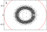
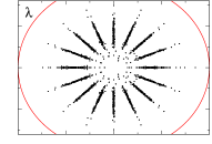
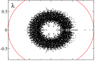
Figure 1: Complex spectrum $\lambda$ of the Ulam matrix approximant $S$ for the Arnold cat map. Top three rows: right column has $N_{x}=47$ and $L=3,4,8$ (from top to bottom); left column has $N_{x}=43$ and $L=3,4,8$ (from top to bottom). Bottom row is for $L=4$ with $N_{x}=50$(left) and $N_{x}=51$ (right). The total matrix size is $N=N_{p}N_{x}$ with $N_{p}=LN_{x}$ and all eigenvalues are shown for each panel. Unit circle is shown in red.

The majority of numerical studies with the Ulam method has been done for one-dimensional maps (see e.g. [14, 15, 17]) but recently the studies were extended to the two-dimensional maps (see e.g. [12, 13, 16, 18]). In a certain respect the interest to such studies was generated by similarities between properties of the Ulam matrix approximant for dynamical maps, which can be viewed as the Ulam networks, and the Google matrix of the World Wide Web as it is discussed in [12, 17]. For 2D dissipative maps it was found that the spectrum is characterized by the fractal Weyl law [12, 18].

In a difference from the previous studies of the Ulam method in 2D maps here we choose the Arnold cat map on a torus of size $L$ since it is fully chaotic, it has well defined diffusive relaxation to the ergodic state at large $L$, and it is time reversible. Thus the aim of this work is to understand the interplay of all these features in the frame of the Ulam method and the finite size Markov chain with the Ulam matrix approximant $S$ generated by this method.

The paper is composed as follows: in Section 2 we describe the properties of spectrum and eigenstates of the matrix $S$, the features of time reversal are analyzed in Section 3 and discussion of the results is presented in Section 4.

2 Spectrum and eigenstates of the Ulam matrix approximant

The complex eigenvalues $\lambda_{i}$ and right eigenvectors $\psi_{i}$ of the Ulam matrix approximant ${\bf S}$ satisfy the equation ${\bf S}\psi_{i}=\lambda_{i}\psi_{i}$ and are determined numerically by direct dioganalization. In agreement with the Perron-Frobenius theorem [8] the maximal eigenvalue is $\lambda_{1}=1$ with the corresponding eigenstate being real, nonnegative and homogeneously distributed over the whole phase space.

The global distributions of eigenvalues $\lambda_{i}$ in the complex plane are shown in Fig. 1 for even and odd number of cells. Usually we keep $N_{p}=LN_{x}$ to have exactly the same amount of cells in each of $L$ sections of the continuous map. The results show that 2D distributions are different for even and prime values of $N_{x}$ (see Fig. 1). For the even case $\lambda$-values are homogeneous inside a circle of a certain radius. For the odd case the distribution has a form of a ring without eigenvalues at $|\lambda|\approx 0$ (or with a smaller density at zero). The arithmetic properties of the number of cells $N_{x}$ and $N_{p}=LN_{x}$ play a visible role. Thus for $N_{x}=47$ we have a formation of star with 16 star rays while for $N_{x}=43$ there are 44 rays which are much less visible (for $N_{x}=37$ we obtain a similar type of distribution with 38 rays). We obtain a similar type of ring spectrum also for $N_{x}=51$ (bottom right panel in Fig. 1). In the case when both $N_{x}$ and $N_{p}$ are primes, e.g. $N_{x}=47$, $N_{p}=191$, (and hence we have only approximate relation $N_{p}\approx LN_{x}$) the visibility of rays also decreases (data not shown).

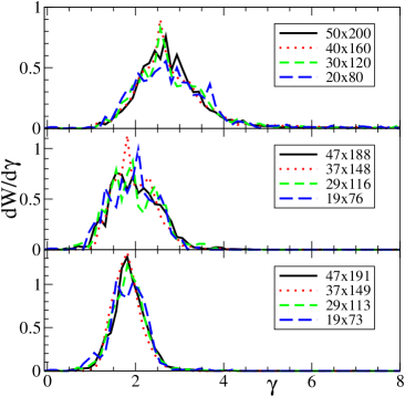
Figure 2: (color online) Dependence of density of states $dW/d\gamma$ on the decay rate $\gamma$ for the Ulam matrix approximant of the cat map with $L=4$. The number of cells $N_{x}$ and $N_{p}$ are even-even on top panel, prime-even on middle panel, and prime-prime on bottom panel. The corresponding values are shown on legends with the notation $N_{x}\times N_{p}$. The densities of states are normalized by the condition $\int_{0}^{10}dW/d\gamma d\gamma=1$.

We expect that in the limit of large $N_{x}$ and $N_{p}=LN_{x}$ with fixed $L$ the distribution will converge to a limiting one in agreement with the spirit of mathematical theorems about the convergence of Ulam matrix approximant for fully chaotic maps [9, 10, 11]. A confirmation of this is seen in Fig. 2 where the density distributions of eigenvalues $dW/d\gamma$ are shown as a function of the relaxation rate $\gamma=-2\ln|\lambda|$. Indeed, the density is essentially size independent showing two distinct distributions for even and odd values of $N_{x}$. We suppose that this difference between two cases can be related to the effect of discretization on the continuous map symmetry $x\rightarrow-x$. The third type of size independent distribution appears in the case of prime values of $N_{x}$ and $N_{p}\approx LN_{x}$ (see Fig. 2) but in this case the difference should be attributed to the fact that this discretization does not preserve exactly $L$ identical classical segments of the continuous map.

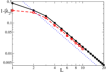
Figure 3: (color online) Spectral gap $\Delta=1-|\lambda_{2}|$ as a function of $L$. Solid (black) and dashed (red) curves represent the cases of $N_{x}=23$ and $N_{x}=47$ respectively; $N_{p}=LN_{x}$. Dotted (blue) line shows the theoretical dependence $\Delta\propto L^{-2}$.

The maximum of the distribution $dW/d\gamma$ is located approximately at $\gamma=2\approx 2h$ corresponding to the value of the Kolmogorov-Sinai entropy $h$. Thus these $\gamma$ values describe the process of exponential divergence of nearby trajectories and are related to the exponential correlations decay generated by chaotic dynamics. In addition to these values $\gamma\sim 1$ there is also the value of $\lambda_{2}=\exp(-\gamma_{2}/2)$ which is positive and is very close to the unit value $\lambda_{1}=1$. It corresponds to the second eigenvalue of the Fokker-Plank equation describing diffusive relaxation to the ergodic steady-state. Indeed, the dependence of the gap $\Delta=1-\lambda_{2}$, shown in Fig. 3, is well in agreement with the dependence (3): a formal fit for $3\leq L$ gives $\Delta\propto 1/L^{\mu}$ with the exponent $\mu=1.97$ for $N_{x}=23$ and $1.94$ for $N_{x}=47$ being close to the theoretical value $\mu=2$. The fit at the fixed exponent $\mu=2$ gives the numerical constant $a$ in the relation $\Delta=a/L^{2}$ being $1.56\pm 0.05$ for $N_{x}=23$ and $1.33\pm 0.05$ for $N_{x}=47$ that is close to the theoretical value $a=2\pi^{2}D=1.64...$. A small deviation can be attributed to the effect of finite size discretization.

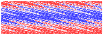
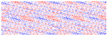
Figure 4: (color online) Eigenstates of the matrix $S$ shown on the whole phase space for $L=4$, $N_{x}=47$ and $N_{p}=LN_{x}$. Top panel shows the eigenfunction $\psi_{2}$, which is real and has $\lambda_{2}=0.917$; middle and bottom panels represent respectively real and imaginary part of the eigenstate $\psi_{27}$ corresponding to the eigenvalue $\lambda_{27}\simeq 0.516+i0.507$. In all panels red corresponds to positive, and blue to negative values. The phase space is rotated on $90$ degrees clockwise so that positive values of $p$ are on the right hand part of the plot.

Two examples of eigenstates $\psi_{2}$ and $\psi_{27}$ of the matrix $S$ are shown in Fig. 4 (the numbering is done in a decreasing order of $|\lambda|$). According to the Fokker-Planck equation (2) we expect to have two double degenerate values of $\lambda_{2}$ with the corresponding running wave eigenstates $\psi_{2}\propto\exp(\pm ik2\pi p/L)$ with $k=\pm 1$ or their liner combination. The numerically found eigenstate $\psi_{2}$ is real up to a numerical level of precision of matrix diagonalization, corresponding to a real $\lambda_{2}$ value. It shows a certain amplitude oscillations along $p$ but its main feature is the sign change along $x$, which is absent in the equation (2). A dependence of eigenstates on $x$ variable remains strongly visible and for other eigenstates (see Fig. 4). For example, the state $\psi_{27}$ has density concentration at points $x=0$ and $x=\pm 0.5$ corresponding to zero force point and discontinuity point respectively.

These results show that the Fokker-Planck equation gives only a fist approximation for the statistical description of dynamics of the Arnold cat map. In contrast to that the Ulam matrix approximant gives much more detailed description. The understanding of all features of this statistical description requires further more detailed studies. We note that according to (2) there should be a series of eigenstates with $\lambda_{k}=\exp(-\Gamma_{D}k^{2})$. We well resolved the case of $k=0,\pm 1$ but we found difficult to define accurately the corresponding higher values. It is possible that they enter rapidly in the dense balk region of ring with many eigenvalues and become mixed with them. Probably larger values of $L$ should be studied to resolve such eigenvalues in a better way. We note that such a series of eigenvalues has been seen for the Chirikov standard map at the critical value of chaos parameter where the diffusion rate is relatively small and thus these eigenvalues are better separated from the balk region [13].

3 Time reversal features and the Ulam time

Even if the exact dynamics is time reversible it becomes easily broken by small errors due to dynamical chaos and exponential instability of motion (see e.g. [5, 19]). In the quantum case the evolution is described by the linear Schrödinger equation that together with the uncertainty principle leads to stability of time reversal in respect to small errors [5, 19, 20]. Let’s now study the time reversal in the frame of the Ulam method where the evolution is described by a linear matrix transformation. For that we start from an initial line in the phase space at $p=0$ with a homogeneous density in $x$, with $w(p,t=0)=1/N_{x}$ and zero otherwise. Then we follow the evolution given by the matrix multiplication $w(p,x,t+1)={\mathbf{S}}w(p,x,t)$ where time $t$ is measured in the number of map iterations $t$. The growth of the second moment $\langle p^{2}(t)\rangle$ as a function of time is shown in Fig. 5. The second moment grows diffusely with time in agreement with the Fokker-Planck equation (2). After $t_{r}$ iterations we perform time reversal by inverting all momenta $p\rightarrow-p$. We see that after $t_{r}$ the second moment $\langle p^{2}(t)\rangle$ starts to decrease during a certain time interval $t_{U}$, where its value becomes minimal, and after that the diffusion restarts again. This time $t_{U}$ is the Ulam time scale during which we have anti-diffusive process which also describes relaxation in a vicinity of big fluctuations [21].

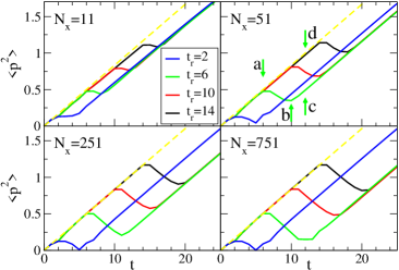
Figure 5: (color online) Time evolution of $\langle p^{2}\rangle$ for an initial distribution with $p=0$ obtained with the Ulam matrix approximant of the Arnold cat map at $L=8$, $N_{p}=LN_{x}$ and $N_{x}=11$ (top-left panel), $51$ (top-right panel), $251$ (bottom-left panel) and $751$ (bottom-right panels). The time inversion is done at $t_{r}=2,6,10,14$. Yellow dashed line shows the theoretical prediction with $\langle p^{2}\rangle=Dt$ and $D=1/12$. The arrows in top-left panel shows the values of time $a,b,c,d$ plotted in Fig. 6.

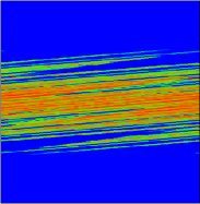
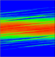
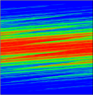
Figure 6: (color online) Time evolution of a $p=0$ state with the Ulam matrix of the Arnold cat map at $L=8$, $N_{x}=51$ and $N_{p}=LN_{x}=408$. Panels show distribution in the whole phase space at the moments of time $a,b,c,d$ marked by arrows in Fig. 5: $(a)$ at $t=6$ (top-left panel); $(b)$ at $t=10$ with $p$-inversion in $t=6$ (top-right panel); $(c)$: $t=12$ with $p$-inversion in $t=6$ (bottom-left panel); $(d)$ at $t=12$ without $p$-inversion (bottom-right panel). Probability density is shown by color with blue for zero density and red for maximal density on a given panel. The values of $\langle p^{2}\rangle$ are marked in green arrows on top-right panel of Fig. 5

The spreading of probability in the whole phase space is displayed in Fig. 6 at different moments of time. These data show that time reversal gives a temporary shrinking of the distribution followed by diffusive spreading continued. Thus the time reversal is preserved only on the Ulam time scale $t_{U}$.

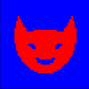
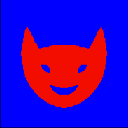
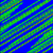
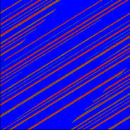
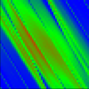
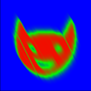
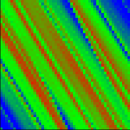
Figure 7: (color online) Evolution of the Arnold cat image generated by the Ulam matrix approximant $S$ with $N_{x}=51$ (left colum) and $N_{x}=751$ (right column) at $L=8$, $N_{p}=LN_{x}$. From top to bottom: initial image $t=0$; image at the moment of time reversal $t=t_{r}=4$; image at the moment of return $t=8$; image at the return moment $t=10$ when the time reversal is made after $t=t_{r}=5$ iterations. Color is proportional to density with blue for zero and red for maximum; only the central initial section $-0.5\leq x<0.5$, $-0.5\leq x<0.5$ is shown.

The strong effects of exponential instability on time reversal breaking are also well seen in Fig. 7. Here, the initial image of the Arnold cat cannot be recovered even if the time reversal is done after only $t_{r}=4$ map iterations for the discretization level with $N_{x}=51$. Only for a much finer discretization level with $N_{x}=751$ the initial image is approximately recovered for $t_{r}=4$ but it degradates rapidly already at time reversal performed after $t_{r}=5$. This illustares the exponentially rapid breaking of time reversal after the Ulam time $t_{U}$.

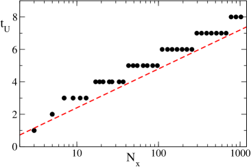
Figure 8: (color online) Dependence of the Ulam time $t_{U}$ with anti-diffusion on the number of cells $N_{x}$ of the Ulam matrix approximant at $L=8$ and $N_{p}=LN_{x}$. An initial state at momentum $p=0$ and homogeneous in $x$ is evolved up to time $t=t_{r}=30$ when a time reversal operation is applied. The dashed line shows the dependence $t_{U}=\ln{N_{x}}/h$

The dependence of the Ulam time $t_{U}$, characterized by the anti-diffusion during time reversal process seen in Fig. 5, on the discretization scale $N_{x}$ is shown in Fig. 8. We see that the results are well described by the dependence

$$t_{U}=\ln N_{x}/h=|\ln\hbar_{eff}|/2h\;,\;\;\hbar_{eff}=1/N_{x}^{2}\;\;,$$ (4)

where $\hbar_{eff}=1/N_{x}^{2}$ can be considered as an effective Planck constant which gives the area of discretized cells. In this form the Ulam time scale $t_{U}$ is similar to the Ehrenfest time $t_{E}$ [22] which appears in the semiclassical limit of systems of quantum chaos. In both cases the mechanism is related to the exponential growth of a wave packet of minimal size with time $\hbar_{eff}\exp(ht)$ due to which the packet size becomes comparable with the whole system size after time $t_{E}$ or in our case after time $t_{U}$.

In spite of this similarity we should note that in the quantum case the time reversal is preserved under rather generic conditions (see [5, 19, 20] and Refs. therein). In contrast to that in the frame of the Ulam method, which also describes the linear matrix evolution, the time reversal is broken after the Ulam time $t_{U}$. The main reason of this difference is related to the fact that the Ulam matrix approximant describes dynamics with eigenvalue modulus smaller than unity while the quantum dynamics is unitary. This result can be also understood from the view point of noise which have a size of discretized cells and which also breaks time reversal.

4 Discussion

In this work we studied the properties of the Ulam matrix approximant $S$, generated by the Ulam method, for the Arnold cat map on a torus of a few integer sections $L$. We show that the spectrum eigenvalues of $S$ converges to a limiting distribution in the limit of small cell discretization and large matrix size $N$. The main part of this spectrum have relaxation rates $\gamma$ with approximate values of the Kolmogorov-Sinai entropy in this system. There are also eigenvalues with much smaller relaxation rate which is in a good agreement with the statistical description by the Fokker-Planck equation.

The continuous model has the property of time reversal but in the frame of the Ulam method the time reversibility is broken on the Ulam time scale $t_{U}$ which grows only logarithmically with the decrease of the cell size in the Ulam method. Such a dependence has certain parallels with that one found for the Ehrenfest time scale in systems of quantum chaos. However, even if in both cases the evolution is described by the linear matrix equations the quantum systems preserves the property of time reversal in presence of weak perturbations, while for the Ulam method the time reversal is broken after the Ulam time scale $t_{U}$. Further studies are required for a better understanding of relations between the spectrum of the Ulam matrix approximant, chaos, diffusion, correlations decay and other statistical properties of dynamical chaos in the Arnold cat map and other chaos systems. Thus this simple model of Vladimir Arnold still keeps its scientific wonder.

Acknowledgments: we thank Elena Chepelianskii for cat image drawing used here and in [5, 19].

References

- [1] V. Arnold, A. Avez, Ergodic problems in classical mechanics, Benjamin, N. Y. (1968).
- [2] I. P. Kornfeld, S. V. Fomin, Ya. G. Sinai, Ergodic theory, Springer, N. Y. (1982).
- [3] B. V. Chirikov, A universal instability of many-dimensional oscillator systems , Phys. Rep. 52 (1979) 263.
- [4] A. Lichtenberg, M. Lieberman, Regular and chaotic dynamics, Springer, N.Y., (1992).
- [5] B. Georgeot and D.L. Shepelyansky, Quantum computer inverting time arrow for macroscopic systems, Eur. Phys. J. D 19 (2002) 263.
- [6] S.M. Ulam, A Collection of mathematical problems, Vol. 8 of Interscience tracs in pure and applied mathematics, Interscience, New York, p. 73 (1960).
- [7] A.A. Markov, Rasprostranenie zakona bol’shih chisel na velichiny, zavisyaschie drug ot druga, Izvestiya Fiziko-matematicheskogo obschestva pri Kazanskom universitete, 2-ya seriya, 15 (1906) 135 (in Russian) [English trans.: Extension of the limit theorems of probability theory to a sum of variables connected in a chain reprinted in Appendix B of: R.A. Howard Dynamic Probabilistic Systems, volume 1: Markov models, Dover Publ. (2007)].
- [8] M. Brin and G. Stuck, Introduction to dynamical systems, Cambridge Univ. Press, Cambridge, UK (2002).
- [9] T.-Y. Li, J. Approx. Theory, Finite approximation for the Perron-–Frobenius operator, a solution to Ulam’s conjecture, 17 (1976) 177.
- [10] M. Blank, G. Keller, and C. Liverani, Ruelle–-Perron–-Frobenius spectrum for Anosov maps, Nonlinearity 15 (2002) 1905.
- [11] D. Terhesiu and G. Froyland, Rigorous numerical approximation of Ruelle–Perron–Frobenius operators and topological pressure of expanding maps, Nonlinearity 21 (2008) 1953.
- [12] D.L.Shepelyansky and O.V.Zhirov, Google matrix, dynamical attractors and Ulam networks, Phys.Rev. E 81 (2010) 036213.
- [13] K.M.Frahm and D.L.Shepelyansky, Ulam method for the Chirikov standard map, Eur. Phys. J. B 76 (2010) 57.
- [14] Z. Kovács and T. Tél, Scaling in multifractals: discretization of an eigenvalue problem, Phys. Rev. A 40 (1989) 4641.
- [15] G. Froyland, R. Murray and D. Terhesiu, Efficient computation of topological entropy, pressure, conformal measures, and equilibrium states in one dimension, Phys. Rev. E 76 (2007) 036702.
- [16] G. Froyland and K. Padberg, Almost–invariant sets and invariant manifolds —- Connecting probabilistic and geometric descriptions of coherent structures in flows, Physica D 238 (2009) 1507.
- [17] L. Ermann and D.L. Shepelyansky, Google matrix and Ulam networks of intermittency maps, Phys. Rev E 81 (2010) 036221.
- [18] L. Ermann and D.L. Shepelyansky, Ulam method and fractal Weyl law for Perron–Frobenius operators, Eur. Phys. J. B 75 (2010) 299.
- [19] B. Georgeot and D.L. Shepelyansky, Stable quantum computation of unstable classical chaos, Phys. Rev. Lett. 86 (2001) 5393.
- [20] D.L. Shepelyansky, Some statistical properties of simple classically stochastic quantum systems, Physica D 8 (1983) 208.
- [21] B.V. Chirikov and O.V. Zhirov, Big entropy fluctuations in statistical equilibrium: the macroscopic kinetics, JETP 93 (2001) 188 [in Russian: Zh. Eksp. Teor. Fiz. 120(1) (2001) 214].
- [22] B.V. Chirikov, F.M. Izrailev and D.L. Shepelyansky, Dynamical stochasticity in classical and quantum mechanics, Sov. Scient. Rev. 2C (1981) 209 [Sec. C - Math. Phys. Rev., Ed. S.P.Novikov vol.2, Harwood Acad. Publ., Chur, Switzerland (1981)]; Quantum chaos: localization vs. ergodicity, Physica D 33 (1988) 77.