Abstract

An algorithm for pose and motion estimation using corresponding features in images and a digital terrain map is proposed. Using a Digital Terrain (or Digital Elevation) Map (DTM/DEM) as a global reference enables recovering the absolute position and orientation of the camera. In order to do this, the DTM is used to formulate a constraint between corresponding features in two consecutive frames. The utilization of data is shown to improve the robustness and accuracy of the inertial navigation algorithm. Extended Kalman filter was used to combine results of inertial navigation algorithm and proposed vision-based navigation algorithm. The feasibility of this algorithms is established through numerical simulations.

0.1 Introduction.

Vision-based algorithms has been a major research issue during the past decades. Two common approaches for the navigation problem are: landmarks and ego-motion integration. In the landmarks approach several features are located on the image-plane and matched to their known 3D location. Using the 2D and 3D data the camera’s pose can be derived. Few examples for such algorithms are [2], [3]. Once the landmarks were found, the pose derivation is simple and can achieve quite accurate estimates. The main difficulty is the detection of the features and their correct matching to the landmarks set.

In ego-motion integration approach the motion of the camera with respect to itself is estimated. The ego-motion can be derived from the optical-flow field, or from instruments such as accelerometers and gyroscopes. Once the ego-motion was obtained, one can integrate this motion to derive the camera’s path. One of the factors that make this approach attractive is that no specific features need to be detected, unlike the previous approach. Several ego-motion estimation algorithms can be found in [4], [5], [6], [7]. The weakness of ego-motion integration comes from the fact that small errors are accumulated during the integration process. Hence, the estimated camera’s path is drifted and the pose estimation accuracy decrease along time. If such approach is used it would be desirable to reduce the drift by activating, once in a while, an additional algorithm that estimates the pose directly. In [8], such navigation-system is being suggested. In that work, like in this work, the drift is being corrected using a Digital Terrain Map (DTM). The DTM is a discrete representation of the observed ground’s topography. It contains the altitude over the sea level of the terrain for each geographical location. In [8] a patch from the ground was reconstructed using ‘structure-from-motion’ (SFM) algorithm and was matched to the DTM in order to derive the camera’s pose. Using SFM algorithm which does not make any use of the information obtained from the DTM but rather bases its estimate on the flow-field alone, positions their technique under the same critique that applies for SFM algorithms [1].

The algorithm presented in this work does not require an intermediate explicit reconstruction of the 3D world. By combining the DTM information directly with the images information it is claimed that the algorithm is well-conditioned and generates accurate estimates for reasonable scenarios and error sources. In the present work this claim is explored by performing an error analysis on the algorithm outlined above. By assuming appropriate characterization of these error sources, a closed form expression for the uncertainty of the pose and motion of the camera is first developed and then the influence of different factors is studied using extensive numerical simulations.

0.2 Problem Definition and Notations.

The problem can be briefly described as follows: At any given time instance $t$, a coordinates system $C(t)$ is fixed to a camera in such a way that the $Z$-axis coincides with the optical-axis and the origin coincides with the camera’s projection center. At that time instance the camera is located at some geographical location $p(t)$ and has a given orientation $R(t)$ with respect to a global coordinates system $W$ ($p(t)$ is a 3D vector, $R(t)$ is an orthonormal rotation matrix). $p(t)$ and $R(t)$ define the transformation from the camera’s frame $C(t)$ to the world’s frame $W$, where if ${}^{\scriptscriptstyle{C}}v$ and ${}^{\scriptscriptstyle{W}}v$ are vectors in $C(t)$ and $W$ respectively, then ${}^{\scriptscriptstyle{W}}v=R(t){}^{\scriptscriptstyle{C}}v+p(t)$.

Consider now two sequential time instances $t_{1}$ and $t_{2}$: the transformation from $C(t_{1})$ to $C(t_{2})$ is given by the translation vector $\Delta p(t_{1},t_{2})$ and the rotation matrix $\Delta R(t_{1},t_{2})$, such that ${}^{\scriptscriptstyle{C\left(t_{2}\right)}}v=\Delta R\left({t_{1},t_{2}}\right){}^{\scriptscriptstyle{C\left(t_{1}\right)}}v+\Delta p\left({t_{1},t_{2}}\right)$. A rough estimate of the camera’s pose at $t_{1}$ and of the ego-motion between the two time instances - $p_{E}(t_{1})$ ,$R_{E}(t_{1})$, $\Delta p_{E}(t_{1},t_{2})$ and $\Delta R_{E}(t_{1},t_{2})$ - are supplied (the subscript letter ‘‘$E$’’ denotes that this is an estimated quantity).

Also supplied is the optical-flow field: $\left\{{u_{i}(t_{k})}\right\}$ (i=1…n, k=1,2). For the $i$’th feature, $u_{i}(t_{1})\in{\mathbb{R}}^{2}$ and $u_{i}(t_{2})\in{\mathbb{R}}^{2}$ represent its locations at the first and second frame respectively.

Using the above notations, the objective of the proposed algorithm is to estimate the true camera’s pose and ego-motion: $p(t_{1})$, $R(t_{1})$, $\Delta p(t_{1},t_{2})$ and $\Delta R(t_{1},t_{2})$, using the optical-flow field $\left\{{u_{i}(t_{k})}\right\}$, the DTM and the initial-guess: $p_{E}(t_{1})$, $R_{E}(t_{1})$, $\Delta p_{E}(t_{1},t_{2})$ and $\Delta R_{E}(t_{1},t_{2})$.

0.3 The Navigation Algorithm

The following section describes a navigation algorithm which estimate the above mentioned parameters. The pose and ego-motion of the camera are derived using a DTM and the optical-flow field of two consecutive frames. Unlike the landmarks approach no specific features should be detected and matched. Only the correspondence between the two consecutive images should be found in order to derive the optical-flow field. As was mentioned in the previous section, a rough estimate of the required parameters is supplied as an input. Nevertheless, since the algorithm only use this input as an initial guess and re-calculate the pose and ego-motion directly, no integration of previous errors will take place and accuracy will be preserved.

The new approach is founded on the following observation. Since the DTM supplies information about the structure of the observed terrain, depth of observed features is being dictated by the camera’s pose. Hence, given the pose and ego-motion of the camera, the optical-flow field can be uniquely determined. The objective of the algorithm will be finding the pose and ego-motion which lead to an optical-flow field as close as possible to the given flow field.

A single vector from the optical-flow field will be used to define a constraint for the camera’s pose and ego-motion. Let ${}^{\scriptscriptstyle{W}}G\in{\mathbb{R}}^{3}$ be a location of a ground feature point in the 3D world. At two different time instances $t_{1}$ and $t_{2}$, this feature point is projected on the image-plane of the camera to the points $u(t_{1})$ and $u(t_{2})$. Assuming a pinhole model for the camera, then $u(t_{1}),u(t_{2})\in{\mathbb{R}}^{2}$. Let ${}^{\scriptscriptstyle{C}}q(t_{1})$and ${}^{\scriptscriptstyle{C}}q(t_{2})$ be the homogeneous representations of these locations. As standard, one can think of these vectors as the vectors from the optical-center of the camera to the projection point on the image plane. Using an initial-guess of the pose of the camera at $t_{1}$, the line passing through $p_{E}(t_{1})$ and ${}^{\scriptscriptstyle{C}}q(t_{1})$ can be intersected with the DTM. Any ray-tracing style algorithm can be used for this purpose. The location of this intersection is denoted as ${}^{\scriptscriptstyle{W}}G_{E}$. The subscript letter ‘‘$E$’’ highlights the fact that this ground-point is the estimated location for the feature point, that in general will be different from the true ground-feature location ${}^{\scriptscriptstyle{W}}G$. The difference between the true and estimated locations is due to two main sources: the error in the initial guess for the pose and the errors in the determination of ${}^{\scriptscriptstyle{W}}G_{E}$ caused by DTM discretization and intrinsic errors. For a reasonable initial-guess and DTM-related errors, the two points ${}^{\scriptscriptstyle{W}}G_{E}$ and ${}^{\scriptscriptstyle{W}}G$ will be close enough so as to allow the linearization of the DTM around ${}^{\scriptscriptstyle{W}}G_{E}$. Denoting by $N$ the normal of the plane tangent to the DTM at the point ${}^{\scriptscriptstyle{W}}G_{E}$, one can write:

$$N^{T}({}^{\scriptscriptstyle{W}}G-{}^{\scriptscriptstyle{W}}G_{E})\approx 0$$ (1)

The true ground feature ${}^{\scriptscriptstyle{W}}G$ can be described using true pose parameters:

$${}^{\scriptscriptstyle{W}}G=R(t_{1})\cdot{}^{\scriptscriptstyle{C}}q(t_{1})\cdot\lambda\;+\;p(t_{1})$$ (2)

Here, $\lambda$ denotes the depth of the feature point (i.e. the distance of the point to the image plane projected on the optical-axis). Replacing (2) in (1):

$$N^{T}(\lambda\cdot R(t_{1})\cdot{}^{\scriptscriptstyle{C}}q(t_{1})\;+\;p(t_{1})\;-\;{}^{\scriptscriptstyle{W}}G_{E})=0$$ (3)

From this expression, the depth of the true feature can be computed using the estimated feature location:

$$\lambda=\frac{N^{T}{}^{\scriptscriptstyle{W}}G_{E}-N^{T}p(t_{1})}{N^{T}R(t_{1}){}^{\scriptscriptstyle{C}}q(t_{1})}$$ (4)

By plugging (4) back into (2) one gets:

$${}^{\scriptscriptstyle{W}}G=R(t_{1}){}^{\scriptscriptstyle{C}}q(t_{1})\cdot\left({\frac{N^{T}{}^{\scriptscriptstyle{W}}G_{E}-N^{T}p(t_{1})}{N^{T}R(t_{1}){}^{\scriptscriptstyle{C}}q(t_{1})}}\right)+p(t_{1})$$ (5)

In order to simplify notations, $R(t_{i})$ will be replaced by $R_{i}$ and likewise for $p(t_{i})$ and $q(t_{i})$ $i=1,2$. $\Delta R(t_{1},t_{2})$ and $\Delta p(t_{1},t_{2})$ will be replaced by $R_{12}$ and $p_{12}$ respectively. The superscript describing the coordinate frame in which the vector is given will also be omitted, except for the cases were special attention needs to be drawn to the frames. Normally, $p_{12}$ and $q$’s are in camera’s frame while the rest of the vectors are given in the world’s frame. Using the simplified notations, (5) can be rewritten as:

$$G\;=\;\frac{R_{1}q_{1}N^{T}}{N^{T}R_{1}q_{1}}G_{E}\;-\;\frac{R_{1}q_{1}N^{T}}{N^{T}R_{1}q_{1}}p_{1}\;+\;p_{1}$$ (6)

In order to obtain simpler expressions, define the following projection operator:

$$\mathcal{P}(u,s)\buildrel\textstyle.\over{=}\left({{\rm I}-\frac{us^{T}}{s^{T}u}}\right)$$ (7)

This operator projects a vector onto the subspace normal to $s$, along the direction of $u$. As an illustration, it is easy to verify that $s^{T}\cdot\mathcal{P}(u,s)v\equiv 0$ and $\mathcal{P}(u,s)u\equiv 0$. By adding and subtracting $G_{E}$ to (6), and after reordering:

$$G=G_{E}+\left[{{\rm I}-\frac{R_{1}q_{1}N^{T}}{N^{T}R_{1}q_{1}}}\right]p_{1}-\left[{{\rm I}-\frac{R_{1}q_{1}N^{T}}{N^{T}R_{1}q_{1}}}\right]G_{E}$$ (8)

Using the projection operator, (8) becomes:

$$G=G_{E}+\mathcal{P}(R_{1}q_{1},N)\left({p_{1}-G_{E}}\right)$$ (9)

The above expression has a clear geometric interpretation (see Fig.1). The vector from $G_{E}$ to $p_{1}$ is being projected onto the tangent plane. The projection is along the direction $R_{1}q_{1}$, which is the direction of the ray from the camera’s optical-center ($p_{1})$, passing through the image feature.

Figure 1: Geometrical description of expression (9) using the projection operator (7)

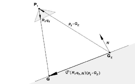
Our next step will be transferring $G$ from the global coordinates frame- $W$ into the first camera’s frame $C_{1}$ and then to the second camera’s frame $C_{2}$. Since $p_{1}$and $R_{1}$describe the transformation from $C_{1}$ into $W$, we will use the inverse transformation:

$${}^{\scriptscriptstyle{C_{2}}}G=p_{12}+R_{12}\left({R_{1}^{T}\left({G-p_{1}}\right)}\right)$$ (10)

Assigning (9) into (10) gives:

$${}^{\scriptscriptstyle{C_{2}}}G=p_{12}+R_{12}\mathcal{L}\left({G_{E}-p_{1}}\right)$$ (11)

$\mathcal{L}$ in the above expression represents:

$$\mathcal{L}=\frac{q_{1}N^{T}}{N^{T}R_{1}q_{1}}$$ (12)

One can think of $\mathcal{L}$ as an operator with inverse characteristic to $\mathcal{P}$: it projects vectors on the ray continuing $R_{1}q_{1}$ along the plane orthogonal to $N$.

$q_{2}$ is the projection of the true ground-feature $G$. Thus, the vectors $q_{2}$ and ${}^{\scriptscriptstyle{C_{2}}}G$ should coincide. This observation can be expressed mathematically by projecting ${}^{\scriptscriptstyle{C_{2}}}G$ on the ray continuation of $q_{2}$:

$${}^{\scriptscriptstyle{C_{2}}}G=\frac{q_{2}}{\left|{q_{2}}\right|}\cdot\left({\frac{q_{2}^{T}}{\left|{q_{2}}\right|}\cdot{}^{\scriptscriptstyle{C_{2}}}G}\right)$$ (13)

In expression (13), ${q_{2}^{T}}\mathord{\left/{\vphantom{{q_{2}^{T}}{\left|{q_{2}}\right|}}}\right.\kern-1.2pt}{\left|{q_{2}}\right|}\cdot{}^{\scriptscriptstyle{C_{2}}}G$ is the magnitude of ${}^{\scriptscriptstyle{C_{2}}}G$’s projection on $q_{2}$. By reorganizing (13) and using the projection operator, we obtain:

$$\left[{{\rm I}-\frac{q_{2}\cdot q_{2}^{T}}{q_{2}^{T}\cdot q_{2}}}\right]\cdot{}^{\scriptscriptstyle{C_{2}}}G\quad=\quad\mathcal{P}(q_{2},q_{2})\cdot{}^{\scriptscriptstyle{C_{2}}}G\quad=\quad 0$$ (14)

${}^{\scriptscriptstyle{C_{2}}}G$ is being projected on the orthogonal complement of $q_{2}$. Since ${}^{\scriptscriptstyle{C_{2}}}G$ and $q_{2}$ should coincide, this projection should yield the zero-vector. Plugging (11) into (14) yields our final constraint:

$$\mathcal{P}(q_{2},q_{2})\left[{p_{12}+R_{12}\mathcal{L}\left({G_{E}-p_{1}}\right)}\right]=0$$ (15)

This constraint involves the position, orientation and the ego-motion defining the two frames of the camera. Although it involves 3D vectors, it is clear that its rank can not exceed two due to the usage of $\mathcal{P}$ which projects ${\mathbb{R}}^{3}$ on a two-dimensional subspace.

Such constraint can be established for each vector in the optical-flow field, until a non-singular system is obtained. Since twelve parameters need to be estimated (six for pose and six for the ego-motion), at least six optical-flow vectors are required for the system solution. But it is correct conclusion for nonlinear problem. If we use Gauss-Newton iterations method and so make linearization of our problem near approximate solution. The found matrix will be always singular for six points (with zero determinant)as numerical simulations demonstrate. So it is necessary to use at least seven points to obtain nonsingular linear approximation. Usually, more vectors will be used in order to define an over-determined system, which will lead to more robust solution. The reader attention is drawn to the fact that a non-linear constraint was obtained. Thus, an iterative scheme will be used in order to solve this system. A robust algorithm which uses Gauss-Newton iterations and M-estimator is described in [9].We begin to use Levenberg-Marquardt method if Gauss-Newton method after several iterations stopped to converge. This two algorithms are realized in lsqnonlin() Matlab function. The applicability, accuracy and robustness of the algorithm was verified though simulations and lab-experiments.

It is more convenient to use more robust for iterations equivalent to (15) equation:

$$\quad\mathcal{P}(q_{2},q_{2})\left[{p_{12}+R_{12}\mathcal{L}_{i}\left({G_{E_{i}}-p_{1}}\right)}\right]/|{}^{\scriptscriptstyle{C_{2}}}G|=0$$ (16)

Using of this normalized form of equations avoids to get incorrect trivial solution when two positions are in a single point on the ground.

0.4 Vision-based navigation algorithm corrections for inertial navigation by help of Kalman filter.

Vision-based navigation algorithms has been a major research issue during the past decades. Algorithm used in this paper is based on foundations of multiple-view geometry and a land map. By help of this method we get position and orientation of a observer camera. On the other hand we obtain the same data from inertial navigation methods. To adjust these two results Kalman filter is used. We employ in this paper extended Kalman filter for nonlinear equations [12].

For inertial navigation computations was used Inertial Navigation System Toolbox for Matlab [13].

Input of Kalman filter consists of two part. The first one is variables $X$ for equations of motion. In our case it is inertial navigation equations. Vector $X$ consists of fifteen components: $[\delta x\>\delta y\>\delta z\>\delta V_{x}\>\delta V_{y}\>\delta V_{z}\>\delta\phi\>\delta\theta\>\delta\psi\>a_{x}\>a_{y}\>a_{z}\>b_{x}\>b_{y}\>b_{z}]$. Coordinates $\delta x\>\delta y\>\delta z$ are defined by difference between real position of the camera and position gotten from inertial navigation calculus.Variables $\delta V_{x}\>\delta V_{y}\>\delta V_{z}$ are defined by difference between real velocity of the camera and velocity gotten from inertial navigation calculus. Variable $\delta\phi\>\delta\theta\>\delta\psi$ are defined as Euler angles of matrix $D_{r}*D_{c}^{T}$ where $D_{r}$ is matrix defined by real Euler angles of camera with respect to Local Level Frame (L-Frame) and $D_{c}$ is matrix defined by Euler angles of camera with respect to Local Level Frame (L-Frame) gotten by inertial navigation computation. It is necessary to pay attention that found Euler angles $\delta\phi\>\delta\theta\>\delta\psi$ ARE NOT equivalent to difference between real Euler angles and Euler angles gotten from inertial navigation calculus. For small values of $\delta\phi\>\delta\theta\>\delta\psi$ perturbations to these angles can be added linearly and so these angles can be used in Kalman filter for small errors. Such choose of angles is made because formulas describing their evolution are much simpler than formulas describing evolution of Euler angles differences. Variables $a_{x}\>a_{y}\>a_{z}$ are defined by vector of Accel bias in inertial navigation measurements.Variables $\>b_{x}\>b_{y}\>b_{z}$ are defined by vector of Gyro bias in inertial navigation measurements.

The second input of Kalman filter is $Z$-result of measurements by vision-based navigation algorithms.Vector $Z$ consists of six components $[\delta x_{m}\>\delta y_{m}\>\delta z_{m}\>\delta\phi_{m}\>\delta\theta_{m}\>\delta\psi_{m}]$Coordinates $\delta x_{m}\>\delta y_{m}\>\delta z_{m}$ are difference between camera position measured by vision-based navigation algorithm and position gotten from inertial navigation calculus.Variable $\delta\theta_{m}\>\delta\psi_{m}$ are defined as Euler angles of matrix $D_{m}*D_{c}^{T}$ where $D_{m}$ is matrix defined by Euler angles of camera with respect to Local Level Frame (L-Frame) measured by vision-based navigation algorithm and $D_{c}$ is matrix defined by Euler angles of camera with respect to Local Level Frame (L-Frame) gotten by inertial navigation computation. Let variable $k$ to be number of step for time discretization used in Kalman filter.

We assume that errors between values gotten by inertial navigation computation and real values are linearly depend on noise. Corespondent process noise covariance matrix is denoted by $Q_{k}$. Diagonal elements of $Q_{k}$ correspondent to velocity are defined by Accel noise and proportional to $dt^{2}$: $Q_{V}\sim dt^{2}$, where $dt$ is time interval between $t_{k}$ and $t_{k-1}$: $dt=t_{k}-t_{k-1}$. Diagonal elements of $Q_{k}$ correspondent to Euler angles are defined by Gyro noise and proportional to $dt$: $Q_{A}\sim dt$.

We assume that errors between values gotten by vision-based navigation algorithm and real values are linearly depend on noise. Corespondent measurement noise covariance matrix is denoted by $R_{k}$. Error analysis giving this matrix is described in [14].

Kalman filter equations describe evolution of $a\>posteriori$ state estimation $X_{k}$ described above and $a\>posteriori$ error covariation covariance matrix $P_{k}$ for variables $X_{k}$.

To write Kalman filter equations we must define two 15x15 matrices yet:$H_{k}$ and $A_{k}$. Matrix $H_{k}$ is measurement Jacobian describing connection between predicted measurement $H_{k}*X_{k}$ and actual measurement $Z_{k}$ defined above. Diagonal elements $H_{k}(1,1)$, $H_{k}(2,2)$, $H_{k}(3,3)$ describing coordinate and elements $H_{k}(4,7)$, $H_{k}(5,8)$, $H_{k}(6,9)$ describing angles are equal to one. The rest of the elements are equal to zero.

$A_{k}$ is Jacobian matrix describing evolution of vector $X_{k}$. The exact expression for this matrix is very difficult so we use approximate formula for $A_{k}$ neglecting by Coriolis effects, Earth rotation and so on. Let $\phi\>\theta\>\psi$ be the Euler angles in L-Frame, $dV$ is deltaV vector gotten from inertial navigation measurements, $f_{vec}$ is acceleration vector in L-frame, $DCM_{\mbox{b-to-l}}$ is direction cosine matrix (from body-frame to L-frame).

The formulas defining $A_{k}$ are follow:

$${\Psi}_{DCM}=\left(\begin{array}[]{ccc}\cos(\psi)&\sin(\psi)&0\\ -\sin(\psi)&\cos(\psi)&0\\ 0&0&1\end{array}\right)$$ (17)

$${\Theta}_{DCM}=\left(\begin{array}[]{ccc}\cos(\theta)&0&-\sin(\theta)\\ 0&1&0\\ \sin(\theta)&0&\cos(\theta)\end{array}\right)$$ (18)

$${\Phi}_{DCM}=\left(\begin{array}[]{ccc}1&0&0\\ 0&\cos(\phi)&\sin(\phi)\\ 0&-\sin(\phi)&\cos(\phi)\end{array}\right)$$ (19)

$$DCM_{\mbox{b-to-l}}=\Phi_{DCM}\Theta_{DCM}\Psi_{DCM}$$ (20)

$$f_{vec}=DCM_{\mbox{b-to-l}}\frac{dV}{dt}$$ (21)

$${Phi(1:3,4:6)}=\left(\begin{array}[]{ccc}1&0&0\\ 0&1&0\\ 0&0&1\end{array}\right)$$ (22)

$${Phi(4:6,7:9)}=\left(\begin{array}[]{ccc}0&-f_{vec}(3)&f_{vec}(2)\\ f_{vec}(3)&0&-f_{vec}(1)\\ -f_{vec}(2)&f_{vec}(1)&0\end{array}\right)$$ (23)

$$Phi(7:9,10:12)=-DCM_{\mbox{b-to-l}}$$ (24)

$$Phi(4:6,13:15)=-DCM_{\mbox{b-to-l}}$$ (25)

The rest of elements for matrix Phi are equal to zero.

$$A_{k}=I+Phi\>dt$$ (26)

Kalman filter time update equations are follow:

$$X_{k}^{-}=[0\>0\>0\>0\>0\>0\>0\>0\>0\>{a_{x}}_{k-1}\>{a_{y}}_{k-1}\>{a_{z}}_{k-1}\>{b_{x}}_{k-1}\>{b_{y}}_{k-1}\>{b_{z}}_{k-1}]$$ (27)

$$P_{k}^{-}=A_{k}P_{k-1}A_{k}^{T}+Q_{k-1}$$ (28)

Kalman filter update equations project the state and covariance estimates from the previous time step $k-1$ to the current time step $k$.

Kalman filter measurement update equations are follow:

$$K_{k}=P_{k}^{-}H_{k}^{T}(H_{k}P_{k}^{-}H_{k}^{T}+R_{k})^{-1}$$ (29)

$$X_{k}=X_{k}^{-}+K_{k}(Z_{k}-H_{k}X_{k}^{-})$$ (30)

$$P_{k}=(I-K_{k}H_{k})P_{k}^{-}(I-K_{k}H_{k})^{T}+K_{k}R_{k}K_{k}^{T}$$ (31)

Kalman filter measurement update equations correct the state and covariance estimates with measurement $Z_{k}$.

The found vector $X_{k}$ is used to update coordinates, velocities, Euler angles, Accel and Gyro biases for inertial navigation calculations on the next step.

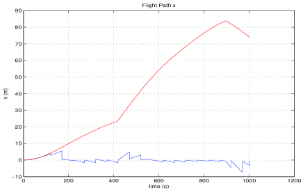
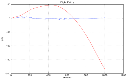
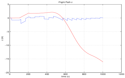
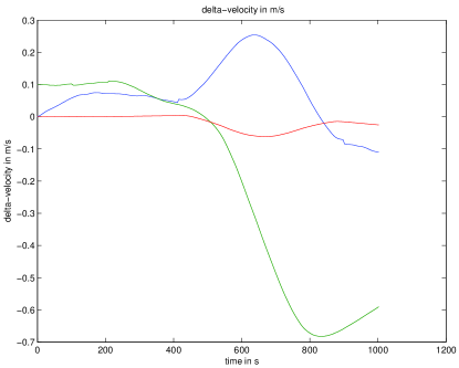
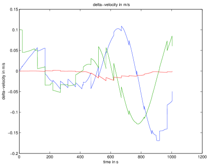
Numerical simulations were realized to examine effectiveness of Kalman filter to combine these two navigation algorithms. On Fig. 2 we can see that corrected path for coordinate error much smaller than inertial navigation coordinate error without Kalman filter. Improved results by help Kalman filter are gotten also for velocity in spite of the fact that this velocity was not measured by help vision-based navigation algorithm Fig. 3.

(a)

(b)

(c)

Figure 2: Position errors ((a) for x coordinate (b) for y coordinate (c) for z coordinate) of the drift path are marked with a red line, and errors of the corrected path are marked with a blue line.

(a)

(b)

Figure 3: (a) Velocity errors of the drift path (x y z components), and (b) Velocity errors of the corrected path (x y z components).

0.5 Conclusions

An algorithm for pose and motion estimation using corresponding features in images and a DTM was presented with using Kalman filter. The DTM served as a global reference and its data was used for recovering the absolute position and orientation of the camera. In numerical simulations position and velocity estimates were found to be sufficiently accurate in order to bound the accumulated errors and to prevent trajectory drifts.

Acknowledgment

We would like to thank Ronen Lerner, Ehud Rivlin and Hector Rotstein for very useful consultations.

Bibliography

- [1] John Oliensis, “A critique of structure-from-motion algorithms”, Computer Vision and Image Understanding, vol. 80, pp. 172–214, 2000
- [2] Y. Liu, M.A. Rodrigues, ‘‘Statistical image analysis for pose estimation without point correspondences’’, Pattern Recognition Letters, vol. 22, pp. 1191-1206, 2001
- [3] P. David, D. DeMenthon, R. Duraiswami, H. Samet, ‘‘SoftPOSIT: Simultaneous pose and correspondence determination’’, ECCV 2002, LNCS 2352, pp. 698-714, 2002
- [4] J. L. Barron and R. Eagleson, ‘‘Recursive estimation of time-varying motion and structure Parameters’’, Pattern Recognition vol. 29, no. 5, pp. 797–818, 1996
- [5] T.Y. Tian, C. Tomashi, D.J. Hegger, ‘‘Comparison of approaches to egomotion computation’’, Department of Psychology and Computer science, Stanford university, CA 94305, 1996
- [6] A.Chiuso, S.Soatto, ‘‘MFm: 3-D Motion From 2-D Motion, Causally integrated over time’’, Washington University Technical Report, 1999
- [7] M. Irani, B. Rousso, S. Peleg, ‘‘Robust Recovery of Ego-Motion’’, Proc. Of CAIP 93, pp. 371-378, 1993
- [8] D.G. Sim, R.H. Park, R.C. Kim, S.U. Lee, I.C. Kim, ‘‘Integrated position estimation using aerial image sequences’’, IEEE transactions on pattern analysis and machine intelligence, vol. 24, no.1, 2002
- [9] Technical report (to be added after the double-blind review).
- [10] R. M. Haralick, ‘‘Propagating Covariance In Computer Vision’’, Advances in Image Understanding, Azriel Rosenfeld, Bowyer and Ahuja, (eds.), IEEE Computer Society Press, pp. 142-157, Washington, 1996
- [11] Rees W.G., ‘‘The accuracy of Digital Elevation Models interpolated to higher resolutions’’, International Journal of Remote Sensing vol. 21 no.1, pp. 7-20, 2000
- [12] Greg Welch and Gary Bishop "An Introduction to the Kalman Filter" UNC-Chapel Hill TR 95-041,NC 27599-3175 April 5, 2004
- [13] www.GPSSoftNav.com
- [14] Oleg Kupervasser, Ronen Lerner, Ehud Rivlin and Hector Rotstein Error Analysis for a Navigation Algorithm based on Optical-Flow and a Digital Terrain Map In the Proceedings of the 2008 IEEE/ION Position, Location and Navigation Symposium, P.1203-1212