Self-interfering matter-wave patterns generated by a moving laser obstacle in a two-dimensional Bose-Einstein condensate inside a power trap cut off by box potential boundaries

Abstract

We report the observation of highly energetic self-interfering matter-wave (SIMW) patterns generated by a moving obstacle in a two-dimensional Bose-Einstein condensate (BEC) inside a power trap cut off by hard-wall box potential boundaries. The obstacle initially excites circular dispersive waves radiating away from the center of the trap which are reflected from hard-wall box boundaries at the edges of the trap. The resulting interference between outgoing waves from the center of the trap and reflected waves from the box boundaries institutes, to the best of our knowledge, unprecedented standing wave patterns. For this purpose we simulated the time dependent Gross-Pitaevskii equation using the split-step Crank-Nicolson method. The obstacle is modelled by a moving impenetrable Gaussian potential barrier. Various trapping geometries are considered.

I Introduction

Recently, there has been considerable interest in the investigation of the effects of a moving obstacle (or object) through a Bose-Einstein condensed system in various trapping geometries B. Jackson, J. F. McCann, and C. S. Adams (1998); P. Engels and C. Atherton (2007); R. Onofrio, C. Raman, J. M. Vogels, J. R. Abo-Shaeer, A. P. Chikkatur, and W. Ketterle (2000); Yu. G. Gladush, A. M. Kamchatnov, Z. Shi, P. G. Kevrekidis, D. J. Frantzeskakis, and B. A. Malomed (2009); T. Winiecki, J. F. McCann, and C. S. Adams (1999); T.-L. Horng, S.-C. Gou, T.-C. Lin, G. A. El, A. P. Itin, and A. M. Kamchatnov (2009); H. Susanto, P. G. Kevrekidis, R. Carretero-Gonz$\acute{a}$lez, B. A. Malomed, D. J. Frantzeskakis, and A. R. Bishop (2007); I. Carusotto, S. X. Hu, L. A. Collins, and A. Smerzi (2006); G. E. Astrakharchik, and L. P. Pitaevskii (2004). The obstacle is a potential barrier generated by a Gaussian laser beam R. Onofrio, C. Raman, J. M. Vogels, J. R. Abo-Shaeer, A. P. Chikkatur, and W. Ketterle (2000); I. Carusotto, S. X. Hu, L. A. Collins, and A. Smerzi (2006), which can be repulsive or attractive depending on the wavelength of the beam. Previous work has also shown that the motion of this obstacle, whether linear or rotational, causes excitations leading to strikingly interesting phenomena such as vortices B. Jackson, J. F. McCann, and C. S. Adams (1998); B. M. Caradoc-Davies, R. J. Ballagh, and K. Burnett (1999); B. M. Caradoc-Davies, R. J. Ballagh, and P. B. Blakie (2000); R. Carretero-Gonz$\acute{a}$lez, P.G. Kevrekidis, D.J. Frantzeskakis, B.A. Malomed, S. Nandi, A.R. Bishop (2007); K.W. Madison, F. Chevy, W. Wohlleben, and J. Dalibard (2000); C. Raman, J. R. Abo-Shaeer, J. M. Vogels, K. Xu, and W. Ketterle (2001), solitons Manjun Ma, R. Carretero-Gonz$\acute{a}$les, P. G. Kevredekis, D. J. Frantzeskakis, and B. A. Malomed (2010); R. Carretero-Gonz$\acute{a}$lez, P.G. Kevrekidis, D.J. Frantzeskakis, B.A. Malomed, S. Nandi, A.R. Bishop (2007), crescent vortex solitons Y. J. He, Boris A. Malomed, Dumitru Mihalache, H. Z. Wang (2008), and dispersive waves accompanying the solitons Vincent Hakim (1997). In addition, there has been growing interest in the investigation of $\check{\hbox{C}}$erenkov radiation H. Susanto, P. G. Kevrekidis, R. Carretero-Gonz$\acute{a}$lez, B. A. Malomed, D. J. Frantzeskakis, and A. R. Bishop (2007); I. Carusotto, S. X. Hu, L. A. Collins, and A. Smerzi (2006) and waves generated by an obstacle moving with supersonic velocity T.-L. Horng, S.-C. Gou, T.-C. Lin, G. A. El, A. P. Itin, and A. M. Kamchatnov (2009); Yu. G. Gladush, A. M. Kamchatnov, Z. Shi, P. G. Kevrekidis, D. J. Frantzeskakis, and B. A. Malomed (2009). However, to the best of our knowledge, none of the previous literature considered the effects of adding a hard-wall to the magnetic trap on the dynamics of the BEC excited by a moving obstacle. It is well known, that vortices can be excited by moving obstacles inside a trapped BEC. However, the parameters used in the present investigation are lower than what is required to obtain significant vortex features, such as the vortex-antivortex pairs observed by Jackson et al. B. Jackson, J. F. McCann, and C. S. Adams (1998).

One goal of this work is to check for a possible existence of vortices in our systems below. Our motivation for this stems from the vast literature on vortices in BECs confined by various traps, with interesting and exciting phenomena both in theoretical B. M. Caradoc-Davies, R. J. Ballagh, and K. Burnett (1999); David L. Feder, Charles W. Clark, and Barry I. Schneider (1999); B. M. Caradoc-Davies, R. J. Ballagh, and P. B. Blakie (2000); S. K. Adhikari and P. Muruganandam (2002); P. Vignolo, R. Fazio, and M. P. Tosi (2007); Daniel S. Goldbaum and Erich J. Mueller (2009); L. Salasnich and B. A. Malomed (2009); M. C. Davis, R. Carretero-González, Z. Shi, K. J. H. Law, P. G. Kevrekidis, and B. P. Anderson (2009); S. K. Adhikari (2010) and experimental domains S. Inouye, S. Gupta, A. P. Chikkatur, A. Görlitz, T. L. Gustavson, A. E. Leanhardt, D. E. Pritchard, and W. Ketterle (2001); S. Tung, V. Schweikhard, and E. A. Cornell (2006); R. A. Williams, S. Al-Assam, and C. J. Foot (2010); T. W. Neely, E. C. Samson, A. S. Bradley, M. J. Davis, and B. P. Anderson (2010).

One way to explore trapped BECs excited by a moving obstacle is by the time-dependent Gross-Pitaevskii equation (TDGPE) whose solutions are known to be solitons T. F. Nonnenmacher and J. D. F. Nonnenmacher (1983) depending on the interactions and certain boundary conditions; the nonlinearity in the GPE being the cause for the appearance of these excitations. The role of the nonlinearity in the generation of solitonic solutions for the nonlinear Schrödinger equation has been studied as early as 1983, when Nonnenmacher and Nonnenmacher T. F. Nonnenmacher and J. D. F. Nonnenmacher (1983) found, that for repulsive interactions no solitons are observed; unlike the case for attractive interactions.

In this work, the split-step Crank-Nicolson method P. Muruganandam and S. K. Adhikari (2009) is applied to numerically solve the two-dimensional (2D${}^{\hbox{al}}$) TDGPE, involving a harmonic or (power-law) PL trap plus a moving obstacle. The trap is cut off by hard-wall box-potential (HWBP) boundaries serving as reflectors of matter waves. In fact, the box potential, along with other hard-wall trapping geometries, has been used previously by Ruostekoski et al. J. Ruostekoski, B. Kneer, W. P. Schleich, and G. Rempe (2001), who explored the interference of a BEC in a hard-wall trap plus the nonlinear Talbot effect. We shall comment on their work in the discussion section. According to Ruostekoski et al., the hard-walls can be realized experimentally by a blue-detuned light sheet. Consequently, the trap is limited by the hard walls and an expanding BEC can be reflected off these walls producing a self-interfering matter-wave (SIMW) field. Essentially, then, we propose an experiment similar to that of Ruostekoski et al., in which we use a 2D${}^{\hbox{al}}$ square box potential. But instead of switching off the isotropic magnetic trap in order to allow the BEC to expand, we excite the BEC by a moving obstacle in order to generate dispersive waves (DWs) that travel towards the hard wall in order to get reflected. Thus, if no DWs are emitted, no SIMWs can be obtained. However, our 2D${}^{\hbox{al}}$ square box is achieved numerically by a different method than that of the latter authors. The main motivation of this work, then, is largely based on the latter work of Ruostekoski et al. J. Ruostekoski, B. Kneer, W. P. Schleich, and G. Rempe (2001). Additional motivation stems from a previous investigation by Jackson et al. B. Jackson, J. F. McCann, and C. S. Adams (1998), who simulated the motion of an “object” through a dilute BEC in a 2D${}^{\hbox{al}}$ harmonic trap, where the object (or obstacle) corresponds to a laser-induced vortex potential. Our goal is to explore the same system of Jackson et al., at a lower mean-field interaction strength ${\cal N}$ but with an additional box-potential trap. We essentially take a closer look at the dynamics of the density surrounding the central BEC at distances larger than $\sim 4$ trap lengths from the center of the trap in the event of matter-wave reflections. Another motivation comes from the work of Hakim Vincent Hakim (1997), who investigated the superflow of a nonlinear Schrödinger fluid past an obstacle. He found that the obstacle repeatedly emits gray solitons which propagate downstream; whereas DWs propagating upstream are emitted at the same time. Since the calculations of Ref.Vincent Hakim (1997) were conducted in 1D and outside a trap, the importance of our current investigation lies, then, in exploring these systems in 2D and further inside various trapping geometries inside a hard wall potential. It is, in fact, the DWs which cause the phenomena obtained in our current study. To this end, we chiefly aim at presenting a phenomenological investigation of SIMW patterns generated by a moving obstacle inside a 2D${}^{\hbox{al}}$ BEC in various trapping geometries surrounded by a HWBP.

Several questions are tackled: First, can we observe DWs in 2D${}^{\hbox{al}}$ harmonically or nonharmonically-trapped BECs excited by a moving obstacle, such as was observed by Hakim Vincent Hakim (1997) for the case of a 1D uniform Bose gas? Second, by adding the HWBP to the harmonic or PL trap, what new features are observed when the latter matter waves are reflected from the hard walls? Will they be similar to Ref.J. Ruostekoski, B. Kneer, W. P. Schleich, and G. Rempe (2001)? Third, how does the energy of the system behave with time? Fourth, what about the momentum density dynamics?

Further, additional simulations of the 1D${}^{\hbox{al}}$ GPE are conducted for the same systems above in an attempt to reproduce the dispersive waves observed by Hakim Vincent Hakim (1997). The purpose is to compare these 1D${}^{\hbox{al}}$ disturbances with the 2D${}^{\hbox{al}}$ disturbances in order to understand their nature in 2D.

Our key results are as follows. i) It is found that in a 2D${}^{\hbox{al}}$ harmonic or PL trap, highly-energetic DWs can be emitted from the moving obstacle. These DWs are highly energetic, capable of surmounting the PL potential barrier to far distances from the trap center. Upon reflection of their wave fronts from the HWBP, their interference with incoming DWs produces at some point perpendicular, 2D${}^{\hbox{al}}$ density-stripes in the matter-wave field, largely influenced by the artefacts of the trapping geometry. This phenomenon has not, to the best of our knowledge, been reported elsewhere to this date; ii) the accompanying energy dynamics of these systems display an oscillatory pattern indicative of a possible presence of solitons; iii) when the trapping strength of the PL is increased, the energy otherwise expended on the creation of the SIMWs is channeled to excite a larger number of solitons inside the trap, eventually leading to a “soliton gas”; iv) the condensate dynamics reveal further an oscillatory behaviour signalling that particles are excited out of and deexcited back into the BEC.

The paper is organized as follows. In Sec.II, we briefly describe the method used. In Sec.III, we present our results, and in Sec.IV we discuss them. The conclusion is presented in Sec.V

II Method

II.1 Time-dependent Gross-Pitaevskii Equation

In this work, we apply the split-step Crank-Nicolson method P. Muruganandam and S. K. Adhikari (2009) to numerically solve the 2D${}^{\hbox{al}}$ TDGPE given by

$$i\hbar\frac{\partial\Psi(\mathbf{r};\tau)}{\partial\tau}\, = \,\left[-\frac{\hbar^{2}}{2m}\left(\frac{\partial^{2}}{\partial x^{2}}\,+\,\frac{\partial^{2}}{\partial y^{2}}\right)\,+\,V(x,y;\tau)\,+\,\right.$$ (1)

$$\left.gN|\Psi(\mathbf{r};\tau)|^{2}\right]\Psi(\mathbf{r};\tau),$$

where $N$ is the number of particles, $g\,\equiv\,4\pi\hbar^{2}a_{s}/m$ is the interaction parameter, with $a_{s}$ the s-wave scattering length in the low-energy and long-wavelength approximation, $m$ is the mass of the boson, and $\hbar$ is Planck’s constant. For the present purposes, $V(x,y;\tau)$ is taken as a potential which varies with time. According to Muruganandam and Adhikari (MA) P. Muruganandam and S. K. Adhikari (2009), the TDGPE can then be recast into a dimensionless form using units of the trap such that

$$\left[-\frac{1}{2}\frac{\partial^{2}}{\partial x^{2}}-\frac{1}{2}\frac{\partial^{2}}{\partial y^{2}}+\tilde{V}(x,y;t)+\right.$$

$$\left.{\cal{N}}|\varphi(x,y;t)|^{2}-i\frac{\partial}{\partial t}\right]\varphi(x,y;t)\,=\,0,$$ (2)

where $t\,=\,\omega_{ho}\tau$ is a unitless time, $\tilde{V}(x,y;t)\,=\,V(x,y;t)/(\hbar\omega_{ho})$ and $x\rightarrow x/\ell$, $y\rightarrow y/\ell$ with $\ell\,=\,\sqrt{\hbar/(m\omega_{ho})}$ the trap length. The parameter ${\cal N}$ is

$${\cal{N}}\,=\,\frac{2Na_{s}}{\ell}\,\sqrt{2\pi\lambda},$$ (3)

$\lambda$ being a parameter describing the width of the ground-state wave function $\phi_{0}(z)\,=\,(\lambda/\pi)^{1/4}\exp(-\lambda z^{2}/2)$ in the $z$-direction, which was then integrated out from the 3D${}^{\hbox{al}}$ wave function so as to get the 2D${}^{\hbox{al}}$ form Eq.(2) above. That is, we consider the $z$-direction to have harmonic confinement of infinite strength. Note further that MA rescaled the wave function using $\varphi(x,y;t)\,=\,\sqrt{\ell^{3}}\Psi(\mathbf{r};\tau)$.

II.2 Trapping potential and moving obstacle

The time-dependent trapping potential is composed of two parts: a static external general 2D${}^{\hbox{al}}$ PL trap $\tilde{V}_{PL}(x,y)$, and a moving potential (MP) barrier (or obstacle) with time $\tilde{V}_{MP}(x,y;\tau)$ which is generated by sweeping a blue-detuned laser beam through the BEC (see, e.g., M. R. Matthews, B. P. Anderson, P. C. Hajlan, D. S. Hall, C. E. Wieman, and E. A. Cornell (1999)). Hence, $\tilde{V}(x,y;t)\,=\,\tilde{V}_{PL}(x,y)\,+\,\tilde{V}_{MP}(x,y;t)$. The PL potential $\tilde{V}_{PL}(x,y)$ is taken to be of the form

$$\tilde{V}_{PL}(x,y)\,=\,\sigma(|x|^{p_{1}}\,+\,\kappa|y|^{p_{2}}),$$ (4)

where $p_{1},\,p_{2}\,>0$ can be any positive numbers, $\kappa$ is an anisotropy parameter, and $\sigma$ is the strength of the PL potential, taken here to be 1. Thus for $p_{1}=p_{2}=2$ we have the usual harmonic trap, whether isotropic ($\kappa=1$) or anisotropic ($\kappa>1$ or $<1$). Both $\sigma$ and $\kappa$ are unitless, since $x$ and $y$ are unitless as well. The goal of using Eq.(4) is to explore the effect of different curvatures of the external trapping potential on the dynamics of a trapped BEC when excited by a moving obstacle.

Next, in order to excite the BEC, we follow Jackson et al. B. Jackson, J. F. McCann, and C. S. Adams (1998) and Bao and Du Weizhu Bao and Qiang Du (2004) and introduce the obstacle in the form of a velocity-dependent Gaussian potential given by

$$\tilde{V}_{MP}(x,y;t)\,=\,A\exp[-\beta x^{2}\,-\,\beta(y\,-\,vt)^{2}],$$ (5)

$A$ being the amplitude, $v$ the velocity in the $y-$direction, and $\beta$ the exponent determining the width.

We further cut off the harmonic or PL trap by a HWBP, which can be numerically achieved by forcing the wave function of the system to vanish at the hard walls. This can be realized by imposing the following boundary conditions

$$\varphi(x,-L_{y}/2;t)\,=\,\varphi(x,L_{y}/2;t)\,=\,0$$

$$\varphi(-L_{x}/2,y;t)\,=\,\varphi(L_{x}/2,y;t)\,=\,0.$$

(6)

Thus the overall trapping geometry is then described by

$$\tilde{V}_{T}(x,y;t)\,=\,$$

$$\left\{\begin{array}[]{l@{\quad:\quad}r}\tilde{V}(x,y;t)&\displaystyle-\frac{L_{x}}{2}<x<\frac{L_{x}}{2};-\frac{L_{y}}{2}<y<\frac{L_{y}}{2}\\ \infty&x\,=\,\pm\displaystyle\frac{L_{x}}{2},y\,=\,\pm\frac{L_{y}}{2}.\end{array}\right.$$ (9)

(10)

We take $L_{x}\,=\,L_{y}\,=\,20$ in trap units. Note that this is different from the way the box potential was constructed in Ref.J. Ruostekoski, B. Kneer, W. P. Schleich, and G. Rempe (2001), where a set of large-amplitude Gaussians was used. In essence, we mimic here an “exact” hard-wall potential where the BEC cannot tunnel $-$even slightly$-$ through the wall.

II.3 Energy functional

The energy is evaluated by the well-known energy functional in trap units

$$E(t)\, = \,\int d^{2}\mathbf{r}\left[\frac{1}{2}|\nabla\varphi(x,y;t)|^{2}\,+\,\tilde{V}(x,y;t)|\varphi(x,y;t)|^{2}\,+\,\right.$$ (11)

$$\left.{\cal{N}}|\varphi(x,y;t)|^{4}\right].$$

Since the above functional includes the moving obstacle Eq.(5), the energy is time-dependent. In fact, an oscillatory pattern is revealed in Sec.III.5.

II.4 Momentum density

In an attempt to investigate the zero-momentum, as well as higher-momentum states, we set out to compute the momentum density of the system given by the Fourier transform

$$\rho_{FT}(k_{x},k_{y};t)\,=\,\frac{1}{4\pi^{2}}\int_{-\infty}^{+\infty}\int_{-\infty}^{+\infty}\rho(x,y;t)e^{ik_{x}x+ik_{y}y}dxdy,$$ (12)

where $\rho(x,y;t)\,\equiv\,|\phi(\mathbf{r};t)|^{2}$ and $(k_{x},k_{y})$ is a 2D${}^{\hbox{al}}$ momentum state. The goal is to explore the dynamics of the condensate fraction as well as the momentum density distribution.

II.5 Numerics and initial conditions

We applied a previously-written Fortran 77 code P. Muruganandam and S. K. Adhikari (2009) to numerically solve Eq.(2) in real time, using the split-step Crank-Nicolson method. For our purposes, we modified the code by including the PL potential Eq.(4) and the moving Gaussian potential Eq.(5), instead of the anisotropic harmonic trap already present in the code. The simulations were conducted on a grid of $400\times 400$ square pixels, the edge of each having the size of a step, 0.05. The time step was chosen to be $\Delta=0.001$. The code has a part which initializes the system and a transient part during which the system evolves. In the initialization step, the nonlinearity is introduced gradually (adiabatically) by a stepwise introduction of the interaction parameter ${\cal N}$ at a rate of $d{\cal N}/dt\,=\,{\cal N}/(N_{stp}\Delta)$, where $N_{stp}$ is the number of time steps $\Delta$ during which the system is initialized. In essence, we modified the initialization part to include a gradual introduction of the Gaussian potential Eq.(5) by a similar gradual increase of its parameters. In fact, we explore in this paper two different initialization conditions via which the obstacle is introduced into the system along with the nonlinearity. It will be later shown, that the generation of DWs depends strongly on the initialization conditions of the system. We find that one condition [(i) below] leads to the generation of DWs, whereas the other [(ii) below] does not. These conditions are as follows:

• Simultaneously with the nonlinearity-introduction, the system is initially subjected to a moving obstacle whose amplitude $A$ and velocity $v$ are gradually increased with time from zero until they reach the desired specific values in this simulation. The corresponding rates are $dA/dt\,=\,A/(N_{stp}\Delta)$ and $dv/dt\,=\,v/(N_{stp}\Delta)$, respectively. At the end of the initialization, the obstacle will have left the center of the BEC. Subsequently, a second equivalent obstacle is again abruptly switched on at the center of the BEC, with the same parameters reached at the end of the previous initialization. Then it is set into motion with speed $v$ until it exits the trap.

• Simultaneously with the nonlinearity-introduction, stationary obstacle is applied in the initialization process, whose amplitude is gradually increased at the rate $A/(N_{stp}\Delta)$. After initialization, the obstacle is set into motion with speed $v$ until it exits the trap.

For the interactions and obstacle we used the parameter values ${\cal N}\,=\,5$, $A\,=\,30$, $\beta\,=\,3$, and $v\,=\,2$. Further, we used $N_{stp}\,=\,42000$ such that the rates $dA/dt$ and $dv/dt$, using $\Delta\,=\,0.001$, are $0.714$ and $0.048$, respectively. Similarly, ${\cal N}$ is gradually increased at a rate of ${\cal N}/(N_{stp}\Delta)\,=\,0.119$. For ⁸⁷Rb atoms with some of the same parameters used in Ref.J. Ruostekoski, B. Kneer, W. P. Schleich, and G. Rempe (2001), i.e., an s-wave scattering length $a_{s}=5.4$ nm and a trapping frequency $\omega_{ho}=2\pi\,\times\,25$ Hz, the trap length $\ell$ is $\sim 2.16\times 10^{4}\,\AA$. If we choose $\lambda=100$ so that the width of the ground state $\phi_{0}(z)$ becomes extremely small along the $z-$axis, one gets $N\sim 40$ particles. If we box length is taken $2L=15\mu\hbox{m}$, then the density of our system is $n\sim\sim N/(4L^{2})=4\times 10^{10}\hbox{m}^{-2}$. Consequently, our systems are in the dilute regime $na_{s}^{2}\sim 10^{-6}$. Ref.J. Ruostekoski, B. Kneer, W. P. Schleich, and G. Rempe (2001) used particle numbers of the order $\sim 10^{3}$, and thus we aim at checking the effect of using a much lower particle number.

Experimentally, then, i) one initially sweeps a very weak laser beam whose intensity and velocity are gradually increasing. After the initialization, when the initial laser beam has left the BEC, a second laser beam is abruptly switched on at the center of the BEC. Then it is set into motion with a constant velocity or acceleration. The second laser beam has the same characteristics as its predecessor at the end of the later initialization. ii) One subjects the system to a stationary laser beam whose intensity is gradually increasing with time. After the intensity has reached a maximum, the laser beam is set into motion with a constant velocity or acceleration.

We therefore propose experiments in which one could try to verify the influence of the latter conditions on the generation of DWs.

III Results

In what follows, we present the results of our simulations. Our major findings are as follows. The moving obstacle inside the BEC generates, in addition to vortices B. Jackson, J. F. McCann, and C. S. Adams (1998); B. M. Caradoc-Davies, R. J. Ballagh, and K. Burnett (1999); B. M. Caradoc-Davies, R. J. Ballagh, and P. B. Blakie (2000); R. Carretero-Gonz$\acute{a}$lez, P.G. Kevrekidis, D.J. Frantzeskakis, B.A. Malomed, S. Nandi, A.R. Bishop (2007); K.W. Madison, F. Chevy, W. Wohlleben, and J. Dalibard (2000); C. Raman, J. R. Abo-Shaeer, J. M. Vogels, K. Xu, and W. Ketterle (2001), 2D${}^{\hbox{al}}$ circular DWs radiating away from the moving obstacle. As their wave fronts reach the hard walls of the box-potential, they are reflected backwards upon which they interfere with incoming circular DWs. This interference creates interesting self-interacting matter-wave (SIMW) patterns. On increasing the powers $p_{1}$ and $p_{2}$ of Eq.(4) to values beyond 2.0, these SIMWs are suppressed. The suppression prevents the energy loss from being carried away by the DWs and saves the energy for another purpose. In the present case, this energy is directed into another channel in which it is expended on exciting a larger number of solitons inside the trap. Similarly, on increasing the anisotropy of the harmonic or PL trap, DWs travelling parallel to the minor axis of the trap, are also suppressed. We have reasons for speculating the presence of real solitons in our systems as opposed to only solitonlike structures reported earlier in Ref.J. Ruostekoski, B. Kneer, W. P. Schleich, and G. Rempe (2001). This is largely supported by the oscillatory behaviour of the energy dynamics indicative of soliton generation N. G. Parker, N. P. Proukakis, and C. S. Adams (2010). By inspecting the density structure at the center of the BEC at some time, the solitons turn out to be of a vortex structure. Finally, the momentum distribution of the system reveals the presence of a zero-momentum condensate density and the condensate fraction oscillates with time. We would like to draw the attention of the reader, that all the upcoming results have been recorded after an initialization process of length $t=4.2$. Thus, when for example a time $t=3$ is mentioned, it refers to the transient time of the simulation. The total simulation time is then 7.2 for this particular case. However, we do not record results in the initialization stage, as we would like to inspect post-initialization phenomena. The following results were obtained using the initial condition (i) in Sec.II.5. It is only in Sec.III.6 that we discuss the effect of condition (ii) in Sec.II.5.

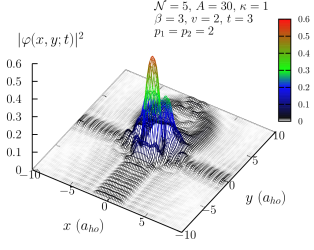
Figure 1: Density of a 2D${}^{\hbox{al}}$ trapped BEC excited by a moving obstacle, Eq.(5), as obtained by a Crank-Nicolson simulation of the 2D${}^{\hbox{al}}$ time-dependent GPE, Eq.(2), at $t=3.0$. The parameters used are ${\cal N}=5.0$, $p_{1}=p_{2}=2.0$, and $\kappa=1.0$. As for the obstacle, Eq.(5), we used $A$=30, $\beta$=3.0, and $v$=2.0. The Fortran program used was that of Adhikari and Muruganandam P. Muruganandam and S. K. Adhikari (2009). Lengths are in units of the trap [$a_{ho}\,=\,\sqrt{\hbar/(m\omega_{ho})}$ ].

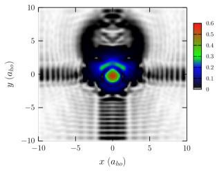
Figure 2: Density map of Fig.   1. Lengths are in units of the trap [$a_{ho}\,=\,\sqrt{\hbar/(m\omega_{ho})}$ ].

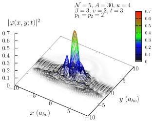
Figure 3: Same as in Fig. 1; but for an anisotropic trap with $\kappa=4.0$ [Eq.(4)]. Lengths are in units of the trap [$a_{ho}\,=\,\sqrt{\hbar/(m\omega_{ho})}$ ].

III.1 Harmonic trap with an obstacle of constant velocity

Figure   1 displays a 2D${}^{\hbox{al}}$ density plot obtained at a transient time of $t=3$ for ${\cal{N}}=5.0$, $p_{1}=p_{2}=2$ (harmonic trap), and $\kappa=1.0$. Fig.  2 displays the corresponding density map. For the obstacle we used $A=30$, $\beta=3.0$, and $v=2.0$. The intriguing result is that four, mutually perpendicular, 2D${}^{\hbox{al}}$ SIMW stripes arise. Two of them propagate parallel to the $x-$axis, the others parallel to the $y-$axis along the motion of the obstacle. In the area surrounding the latter cross-like pattern, some residual faint interference pattern is also present. We shall relate this phenomenon to an artefact of the trapping geometry discussed later in Sec. IV.2. It is noted that the SIMW stripes generated in the regime $y>0$ are perturbed by the obstacle causing the density depression (small valley) in the upstream direction, behind the central BEC peak at $t=3$. Further, upon a closer inspection of the area surrounding the small moving “valley” in the upper part of Fig.  2, a pair of “holes” can be seen identifying a pair of vortices. This valley displays also a complex structure which could be due to vortex excitations. It should be recalled that the motion of the obstacle is in the positive $y-$direction. For further demonstration, see the movie in the supplementary material section mov (a) corresponding to the time evolution of $|\varphi(x,y;t)|^{2}$ in Fig.  1. Upon a careful inspection of the movie, one can see a solitonlike structure in the matter-wave field upon the reflection of the BEC from the hard walls, similar to what has been reported by Ref.J. Ruostekoski, B. Kneer, W. P. Schleich, and G. Rempe (2001).

Figure   3 displays the 2D${}^{\hbox{al}}$ density for the same parameters as in Fig.  1, except that the trap is now anisotropic with $\kappa=4$, with $x$ the major and $y$ the minor axis. Because of a stronger confinement along the $y-$axis, 2D${}^{\hbox{al}}$ SIMW stripes are absent in that direction, as outgoing matter waves from the obstacle are suppressed, unable to tunnel through the potential barrier. Rather, they are observed to emerge only along the positive $x-$axis. There is another matter wave emerging parallel to the 2D${}^{\hbox{al}}$ SIMW in Fig.  3, which has a larger wavelength and therefore less energy than the accompanying SIMW.

In Fig.  4, a magnified view of a section of the SIMW stripes appearing in Fig.  1 is presented. Apparently, the SIMWs eventually propagate almost without a significant change in width or amplitude. Further, they display a peculiar complex structure. Another magnified view of a section of the SIMWs of the anisotropic case of Fig.  3 is displayed in Fig.  5. This time, two separate wave structures are revealed. One is the SIMW centered along the $y=0$ axis; the other is a decaying matter wave of a larger wave length centered along the $y=-4$ axis. The latter second wave decays after a certain distance ($\sim$ 10 trap lengths) from $x=0$ and is therefore less energetic than the DWs.

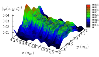
Figure 4: Magnified section of the SIMW stripes appearing in Fig.  1, showing how these waves propagate. Lengths are in trap units [$a_{ho}\,=\,\sqrt{\hbar/(m\omega_{ho})}$].

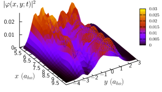
Figure 5: Same as in Fig.  4; but for Fig.  3 with $\kappa$=4.0. There are now two separate wave structures. One centered along the $y=0$ axis which is a SIMW; the other along the $y=-4$ axis. Lengths are in trap units [$a_{ho}\,=\,\sqrt{\hbar/(m\omega_{ho})}$].

III.2 Harmonic trap with an accelerated obstacle

The purpose of this section is to demonstrate that 2D${}^{\hbox{al}}$ SIMW stripes can still be generated by applying an accelerated obstacle (AO). For this purpose, a variant of the Gaussian potential [Eq.(5)] is introduced, where the velocity term is replaced by an acceleration term $(1/2)at^{2}$:

$$\tilde{V}_{AO}\,=\,A\exp\left[-\beta x^{2}\,-\,\beta\left(y-\frac{1}{2}at^{2}\right)^{2}\right],$$ (13)

where $a$ is the acceleration of the potential. Another goal is to display the effect of the “force” of an obstacle on the dynamics of a 2D${}^{\hbox{al}}$ trapped BEC. The obstacle has a “mass”, as has been outlined earlier by Astrakharchik and Pitaevskii G. E. Astrakharchik, and L. P. Pitaevskii (2004), and might therefore be able to produce a shock wave when accelerated.

Figure 6 displays the resulting density plot at $t=3$ for the same parameters as in Fig.  1, except that we are using the AO Eq.(13) with $a=1$ instead of Eq.(5). It can be seen that, again similarly to Fig.  1, a perpendicular set of 2D${}^{\hbox{al}}$ SIMW stripes is observed. As a result, one concludes that an accelerated obstacle is also able to generate 2D${}^{\hbox{al}}$ SIMW stripes in a 2D${}^{\hbox{al}}$ trapped BEC.

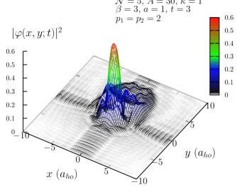
Figure 6: Same as in Fig.   1; but with an accelerated obstacle with $a=1.0$ [cf. Eq.(13)].

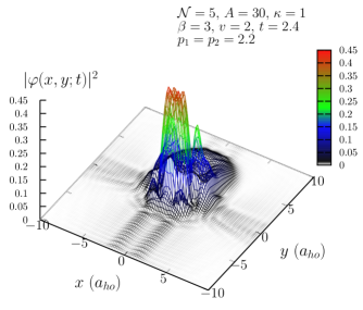
Figure 7: Same as in Fig.  1; but for $p_{1}=p_{2}$=2.2 at $t=2.4$. Lengths are in units of the trap [$a_{ho}\,=\,\sqrt{\hbar/(m\omega_{ho})}$].

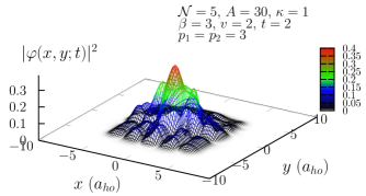
Figure 8: Same as in Fig. 1; but for $p_{1}=p_{2}=3.0$ at $t=2.0$. Lengths are in units of the trap [$a_{ho}\,=\,\sqrt{\hbar/(m\omega_{ho})}$].

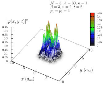
Figure 9: Same as in Fig. 1; but for $p_{1}=p_{2}=4.0$ at $t=2.0$. Lengths are in units of the trap [$a_{ho}\,=\,\sqrt{\hbar/(m\omega_{ho})}$].

III.3 Nonharmonic potentials: effect of trap curvature

In this section, we explore whether one can still obtain 2D${}^{\hbox{al}}$ SIMW stripes if one uses a stronger PL trap with $p_{1}$, $p_{2}\,>\,2$. It was found that for a choice of $p_{1}=p_{2}=2.2$, one still obtains these stripes similar to Fig.  1, as displayed in Fig.  7. However, a closer inspection of the latter figure reveals a pair of parallel stripes propagating downstream along the negative $y-$axis. The parameters are the same as those used in Fig.  1, except for $p_{1}$ and $p_{2}$. The intensity of the 2D${}^{\hbox{al}}$ SIMW stripes is, however, smaller parallel to the $x-$axis than the $y-$axis. On going up to larger powers, $p_{1}=p_{2}\geq 3$, the 2D${}^{\hbox{al}}$ SIMW stripes are suppressed as displayed in Figs.  8 and 9. The curvature at the edges of the trap plays a crucial role in the suppression of the SIMWs as explained later in Sec. IV.

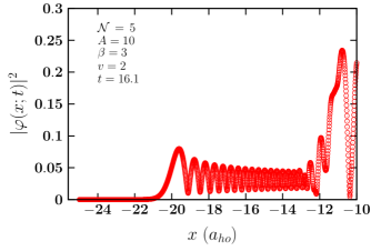
Figure 10: One-dimensional SIMWs generated by a 1D${}^{\hbox{al}}$ Crank-Nicolson simulation of the time-dependent GPE Eq.(14). The system is a 1D${}^{\hbox{al}}$ hard-sphere Bose gas of ${\cal N}=5$. The vortex potential parameters are $A=10$, $\beta=3$, and $v=2$. Parameters and lengths are in trap units [$a_{ho}\,=\,\sqrt{\hbar/(m\omega_{ho})}$].

III.4 One-dimensional simulations

In this section, we present additional results of the Crank-Nicolson simulation of the 1D${}^{\hbox{al}}$ GPE, i.e., the 1D${}^{\hbox{al}}$ version of Eq.(2):

$$\left[-\frac{1}{2}\frac{\partial^{2}}{\partial x^{2}}\,+\,\tilde{V}(x;t)\,+\,{\cal N}|\varphi(x;t)|^{2}\,-\,i\frac{\partial}{\partial t}\right]\varphi(x;t)\,=\,0,$$ (14)

where

$$\tilde{V}(x;t)\,=\,\frac{1}{2}x^{2}\,+\,A\exp[-\beta(x\,-\,vt)^{2}],$$ (15)

and the velocity $v$ is directed along the $x-$axis. Further, as in the 2D${}^{\hbox{al}}$ case, the harmonic trap is cut off by a 1D HWBP such that

$$\varphi(-L_{x};t)\,=\,\varphi(L_{x};t)\,=\,0.$$ (16)

The goal is to provide additional support for our arguments made about the nature of the observed 2D${}^{\hbox{al}}$ SIMW stripes.

Figure    10 demonstrates the density $|\varphi(x;t)|^{2}$ at a time $t=16.1$ for ${\cal N}=5$, $A=10$, $\beta=3$, and $v=2$. One can see an SIMW emitted to the left of the central BEC density travelling along the $-x$ direction. The sharp dip in the density near $x=-10$ is a dark soliton excited by the moving obstacle. The DW was able to climb up the external potential barrier up to a distance of $\sim 20$ trap lengths from the center of the trap! Amazingly, these waves are largely energized, enough to travel that far from the center of the trap. Given for example a distance of $x\,=\,20a_{ho}$, one estimates this wave must have an energy of at least $200\hbar\omega_{ho}$. Hence, a question arises whether the moving obstacle is indeed the mechanism which would impart such a high energy to these excitations. In fact, if one were to compute the “mass” of the obstacle and calculate the associated kinetic energy, one would then verify this fact. Thus, let us make the following estimation: If the “mass” of an obstacle is $m$ and its velocity $v$, then by assuming the obstacle imparts all its kinetic energy to the outgoing 1D${}^{\hbox{al}}$ dispersive waves from the trap center, these waves need an energy of $(1/2)mv^{2}\sim 200\hbar\omega_{ho}$ to climb up the external harmonic barrier a distance $x=20a_{ho}$, before getting reflected back from the box potential. Accordingly, if $v=2$, then $m\sim 100m_{B}$, where $m_{B}$ is the boson mass incorporated in the trap length $a_{ho}=\sqrt{\hbar/(m_{B}\omega_{ho}})$. That is, the obstacle posesses a large mass equivalent to the mass of $\sim 100$ bosons, all moving at $v=2$. Given the latter mass, one can conclude that the moving obstacle is able to impart very high energies to the system, exciting dispersive waves able to surmount the external potential barrier to extremely large distances!

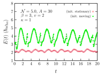
Figure 11: Dynamics of the energy $\langle E(t)\rangle$ [Eq.(11)] of the system in Fig.  1 [solid circles, initial condition (i)]. The open circles are for Fig.  14 below with initial condition (ii). Energies are in trap units ($\hbar\omega_{ho}$).

III.5 Energy Dynamics

In this section, we display the time-dependence of the energy functional [Eq.(11)] for the systems considered in the previous sections. The goal is to present evidence for a possible existence of solitons inside the 2D${}^{\hbox{al}}$ trapped BEC excited by a moving obstacle, based on the fact that the time-dependence of the energy is oscillatory for solitons N. G. Parker, N. P. Proukakis, and C. S. Adams (2010). First, we present Fig.  11 which displays the energy dynamics for the system of Fig.  1 [solid circles, initial condition (i)]. The solid circles are for Fig.  14 below with initial condition (ii) added here for the purpose of comparison. The energy $E(t)$ [Eq.(11)] fluctuates in time about a seemingly stable time average; this is indicative of the presence of solitons in the system N. G. Parker, N. P. Proukakis, and C. S. Adams (2010). It can also be argued that the system is emitting and reabsorbing energy.

Figure  12 displays the energy dynamics for the anisotropic system of Fig.  3, and Fig.  13 the energy dynamics for the systems in the different trapping geometries of Figs.  7-9, with $p_{1}=p_{2}=2.2$ (open circles), $p_{1}\,=\,p_{2}\,=3.0$ (solid circles), and $p_{1}=p_{2}=4$ (open triangles), respectively. Fig.  12 reveals a more rapid and spikier behavior in the energy oscillations than the other two figures. The system in an anisotropic trap thus tends to emit and absorb energy at a faster rate than in an isotropic trap. Fig.  13 displays the effect of the trap curvature on the energy oscillatory patterns. Note that the oscillatory behavior becomes more irregular as the power of the trap is increased via $p_{1}$ and $p_{2}$. In fact, the energy seems to become almost stable with time when $t>4$ for $p_{1}=p_{2}=2.2$ and 3.

Next we proceeded to determine the role of the moving obstacle and the nonlinearity of the TDGPE in the observed energy oscillations. We therefore checked the time-dependence of the energy, Eq.(11) for two cases: 1) in the absence of the obstacle and the presence of the nonlinearity and 2) vice versa. In case (1) the system reached equilibrium immediately after the initialization process and stopped evolving. No SIMWs were observed whatsoever as the BEC is neither excited nor is the magnetic trap switched off to allow its expansion. The energy and density pattern stabilized with time as well. No energy oscillations were observed. However, in case (2), SIMWs were generated. The system and energy were still evolving after the initialization process and the energy displayed oscillations. Therefore, the main source for the observed oscillations is the moving obstacle. Consequently, the moving obstacle not only generates the 2D${}^{\hbox{al}}$ SIMW stripes observed in Figs.  1, 3, 6, and 7-9, but also solitons inside the central part of the BEC.

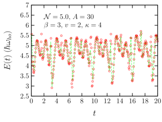
Figure 12: As in Fig.  11; but for the system in Fig.  3. Energies are in units of the trap $\hbar\omega_{ho}$.

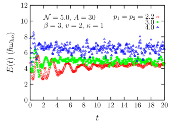
Figure 13: Dynamics of the energy $\langle E(t)\rangle$ [Eq.(11)] for various trapping geometries: open circles: $p_{1}=p_{2}=2.2$, system of Fig.  7; solid circles: $p_{1}=p_{2}=3$, system of Fig.  8; open triangles: $p_{1}=p_{2}=4.0$, system of Fig.  9. Energies are in units of the trap $\hbar\omega_{ho}$.

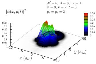
Figure 14: As in Fig.  1; but using the initial conditions (ii) in Sec.II.5.

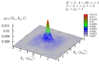
Figure 15: Momentum density distribution of the system in Fig.  1 obtained by the Fourier transform Eq.(12). Wave vectors $k_{x}$ and $k_{y}$ are in units of the trap ($a_{ho}^{-1}$).

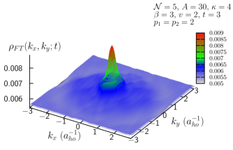
Figure 16: As in Fig.  1; but for the system of Fig.  3.

III.6 Alternative initial conditions

Here, we demonstrate the effect of using the alternative initial condition (ii) presented in Sec. II.5. This is when the laser potential (obstacle) is initially kept stationary, while its intensity is gradually increased up to a certain chosen maximum. After this maximum is reached, it is set into motion. The resulting density at $t=3$ is shown in Fig.  14 which is practically the same as Fig.  1, but using the alternative initial condition (ii) in Sec.II.5. The previously-observed SIMW pattern is not obtained at $t=3$, even at later times (not shown). This result holds similary for the anisotropic case tackled earlier in Fig.  3. Consequently, one can argue a very peculiar result, which shows that generation of SIMWs is dependent on the initial conditions of an excited BEC. We would also like to note that the energy of this system displays an oscillatory behaviour as well (as shown in Fig.  11 (open circles)). Henceforth, the observed energy oscillations are not a result of specific initialization conditions.

III.7 Dynamics of momentum density

Here we try to detect the condensate in order to explore its dynamics. For this purpose, the time dependent momentum density is computed from the Fourier transform of the spatial density $\rho(x,y;t)$, as given by Eq.(12).

Figures 15-17 display the momentum density $\rho_{FT}(k_{x},k_{y};t)$ of Figs.  1, 3, and 7, respectively, and at the indicated times $t$. In all the latter momentum density figures, there exists a Gaussian-like, zero-momentum density peak centered at $(k_{x},k_{y})\equiv(0,0)$. The smoothness of this peak and the surrounding density in $k-$space indicate that the BEC excitations in Figs.  15-17 occur in a continuous band of $(k_{x},k_{y})$ states. In fact the regime around the central BEC peak, so to speak, displays a nonzero momentum density surface. By inspecting Fig.  15 closely, one can observe some rectangular-like momentum-density wave structure surrounding the central BEC peak. In other words, the effects of the geometry-artefact (see Sec. IV.2) are manifested even in the $k-$space of the current system. Fig.  16 shows no specific structure around the central peak, but rather a smooth momentum density distribution. Nevertheless, and upon a close inspection of the momentum density along the $k_{x}=\pm 3$ lines in the neighborhood of $k_{y}=0$, some depression in the density is observed as indicated by a slight bending in the plane. Fig.  17 on the other hand displays some valleyed structure in the vicinity of the zero-momentum peak.

Throughout the evolution of the system, the central BEC peak neither disappears nor does it expand significantly, although it fluctuates in amplitude. Consequently, the zero-momentum condensate density $\rho_{FT}(0,0;t)$ displays oscillatory patterns shown in Fig.  18 corresponding to the latter systems. Fig.  15: (open circles) $\kappa=1$, $p_{1}=p_{2}=2$; Fig.  16: (solid circles) $\kappa=4$, $p_{1}=p_{2}=2$; Fig.  17: (open triangles) $\kappa=1$, $p_{1}=p_{2}=2.2$. The oscillations in $\rho_{FT}(0,0;t)$ are a strong indication to particles being excited out of the condensate as $\rho_{FT}(0,0;t)$ decreases, and particles “falling back” into the condensate as $\rho_{FT}(0,0;t)$ rises again. Therefore the presence of SIMW phenomena seems to promote excitations out of and deexcitations back into the condensate. For further visual demonstration of the momentum dynamics of the system, see the movie in the supplementary material section mov (b), which corresponds to Fig.  15. Further, one must note that the condensate oscillations are substantially damped in the range $8\stackrel{{\scriptstyle<}}{{\sim}}t\stackrel{{\scriptstyle<}}{{\sim}}18$ for $p_{1}=p_{2}=2.2$.

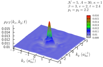
Figure 17: As in Fig.  1; but for the system of Fig.  7.

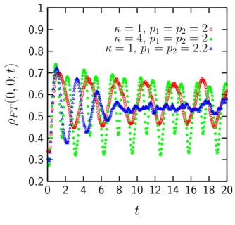
Figure 18: Dynamics of the zero-momentum density $\rho(0,0;\tau)$ for the systems of Fig.  1 with $\kappa=1$, $p_{1}=p_{2}=2$ (open circles); Fig.  3 with $\kappa=4$, $p_{1}=p_{2}=2$ (solid circles); and Fig.  7 with $\kappa=4$, $p_{1}=p_{2}=2.2$ (open triangles), respectively.

IV Discussion

We now set out to find an explanation for the cross-like 2D${}^{\hbox{al}}$ SIMW stripes observed in Figs.  1, 6, and 7. In addition, we discuss briefly the work of Ruostekoski et al. J. Ruostekoski, B. Kneer, W. P. Schleich, and G. Rempe (2001), the analogy with 1D^al dispersive waves, backflow, and a possible existence for vortices and solitons.

IV.1 Work of Ruostekoski et al. J. Ruostekoski, B. Kneer, W. P. Schleich, and G. Rempe (2001)

Ruostekoski et al. J. Ruostekoski, B. Kneer, W. P. Schleich, and G. Rempe (2001) explored the self-interference of BEC matter-waves in hard-wall traps of several geometries. Their work is very much related to ours and it provides significant results. According to these authors, the hard walls can be realized by the application of blue-detuned far-off resonant laser-light sheets. Their goal was to study the evolution of a BEC upon the reflection of these matter-waves from the hard-walls. Particularly, the nonlinear Talbot effect was investigated in a 1D hard-wall trap, where solitonlike structures were obtained. It was noted, that the nonlinear Talbot effect of a coherent matter-wave field is analogous to the Fresnel diffraction effect in optics. Similarly, we can argue that the cross-like matter-wave pattern observed in our Fig.  1 above, is also analogous to the Fraunhofer diffraction pattern M. van der Poel, C.V. Nielsen, M.-A. Gearba, and N. Andersen (2001).

In general, they initially confined the system in a magnetic field trap added to the hard-wall potential. Upon switching off the magnetic trap, the BEC expanded and was reflected from the hard-wall boundaries causing a self-interference pattern. Ruostekoski et al. conducted these investigations in (i) a 1D box with an isotropic magnetic trap; (ii) a 3D${}^{\hbox{al}}$ highly anisotropic cigar trap with hard-walls introduced by laser-light sheets in the axial direction of the trap; (iii) a 2D${}^{\hbox{al}}$ circular boundary, and (iv) a 2D${}^{\hbox{al}}$ square box, both of them with isotropic traps. In (i), a complex self-interference pattern is obtained in the time evolution of the BEC density, characterized by canals corresponding to the evolution of solitonlike structures. This is where the Talbot effect was observed. The “density holes” observed in the density-dynamics corresponded to a gray solitonlike structure. A similar solitonlike structure is obtained in the second case (ii) of the cigar trap, though with some differences. In case (iii), the system is investigated for two subcases: initially symmetric, and with an initial broken symmetry. In the former ring solitons are observed, in the latter the solitonlike structures break and form vorticity. In (iv), the reflections of the matter-waves result also in solitonlike structures.

The main difference between our work and that of Ruostekoski et al. is that we do not switch off the magnetic trap, but rather we excite the BEC by a moving laser-potential. In addition, we needed to apply certain initial conditions in order to cause an excitation of dispersive waves. Another difference is, whereas the latter authors observe the Fresnel diffraction effect in the 2D${}^{\hbox{al}}$ square box potential, we are able to obtain cross-like matter-wave patterns analogous to a Fraunhofer diffraction pattern. In addition, we would like to emphasize that we have focused here on the energy and momentum dynamics of the BEC matter-wave field.

IV.2 Artefact of the Geometry

According to Ref.J. Ruostekoski, B. Kneer, W. P. Schleich, and G. Rempe (2001), then, the rectangular pattern of the waves observed in Figs.  1, 3, 6, and 7 is due to the nature of the boundary conditions imposed on the wave function at the edges of the square mesh during the simulation. Our boundary conditions Eq.(6) force the wave function to vanish there, thus mimicing an impenetrable hard wall. According to Eq.(10), one can see that into this box there is embedded the 2D${}^{\hbox{al}}$ harmonic oscillator (or PL) trap, both of which share the same center. The hard walls of the box are parallel to the coordinate axes $x$ and $y$ and the harmonic (or PL) trap ends where the hard walls begin and cannot reach beyond. Yet, the motion of the obstacle energizes the system to such an extent producing waves capable of reaching the edges of the square mesh, but not farther than this. At the hard walls the wave function of the system vanishes and $-$possessing enough energy$-$ it is reflected from the HWBP. As a result, a self-interfering matter-wave pattern forms, as waves outgoing from the trap center interfere with “incoming” waves reflected from the hard walls. Inspect also carefully our movie in the supplementary section mov (a). The perpendicular 2D${}^{\hbox{al}}$ SIMWs observed are a result of a trapping geometry-artefact arising from the inner curvature of the magnetic trap (PL trap), the HWBP, and the finite width of the central BEC peak from which the outgoing DWs are emitted. The presence of a moving density dip due to the obtacle is largely responsible for the presence of this cross-like SIMW pattern. Further, one can argue similarly to Ref.J. Ruostekoski, B. Kneer, W. P. Schleich, and G. Rempe (2001) that the latter cross-like patterns is a result of an initial symmetry breaking of the system caused by an initial slight displacement via the moving obstacle. On the other hand, the pair of parallel stripes observed in Fig.  7 is most likely due to the emission of a pair of nonconcentric circular DWs from the central BEC peak, each of which is reflected from the hard wall, creating its own SIMW pattern.

Now when the trap is strengthened by increasing its power exponents, i.e., by setting $p_{1}$ and $p_{2}$ larger than 2.2 in Eq.(4), the expanding BEC waves do not reach the HWBP anymore and rather decay by tunneling through the edges of the PL trap. As a result, no SIMW patterns are formed in Figs.  8 and 9.

IV.3 Analogy with 1D${}^{\hbox{al}}$ dispersive waves

We consider an investigation by Hakim Vincent Hakim (1997), which carries some similar features to ours. He explored the flow of a nonlinear Schrödinger fluid past an immobile obstacle in a one dimensional homogeneous Bose gas and found that the obstacle repeatedly emitted gray solitons propagating downstream, i.e., opposite to the motion of the fluid. At the same time he observed upstream propagating dispersive waves, i.e., in the direction of fluid flow. We can, therefore, explain the initial emission of waves from the center of the trap, and before they are reflected from the HWBP, based on an analogy with Hakim’s investigation. Hakim Vincent Hakim (1997) demonstrated the excitation of dispersive waves (DWs) in a 1D${}^{\hbox{al}}$ uniform Bose gas in the direction of obstacle motion or fluid flow. Basing on Hakim’s results, we could then argue that the waves emitted from the trap center in our 2D${}^{\hbox{al}}$ system are similarly circular DWs. Consequently, an outgoing circular DW interferes with an “incoming” linear DW reflected off the box-potential boundaries. However, the cross-like pattern observed is a peculiar result which, to the best of our knowledge, has not been reported elsewhere.

IV.4 Vortices and solitons

On inspecting Fig.  1 closely, one can see two cylindrical, mantel-like walls surrounding the central BEC peak. The region between each “mantel” and the central BEC peak displays a deep density depression which is reminiscent of crescent vortex solitons Y. J. He, Boris A. Malomed, Dumitru Mihalache, H. Z. Wang (2008). There is a mantel in the front of the central peak (in the region $y<0$) and in the back (at $y>0$). In addition, the pair of “holes” which was indicated to earlier in Sec.III.1, is a vortex anti-vortex pair similar to the one observed by Jackson et al. B. Jackson, J. F. McCann, and C. S. Adams (1998) except that in our pair the vortices are much smaller. It is anticipated that vortex excitations could play a role in exciting DWs in 2D${}^{\hbox{al}}$ systems. Indeed, the oscillating feature of the energy dynamics shown in Figs.  11-13 is a manifestation of solitonic presence inside the trap. According to Parker et al. N. G. Parker, N. P. Proukakis, and C. S. Adams (2010), the energy of a soliton is oscillatory; this supports our previous conclusion regarding the possible presence of vortex solitons at some instant of time in Fig.  1.

IV.5 Suppression of dispersive-waves and soliton generation

Dispersive waves are suppressed in an anisotropic trap along the strongly-confining direction, as displayed in Fig.  3; whereas they are still emitted along the major axis of the elongated trap. The dispersive waves do not have enough kinetic energy to climb up the external potential barrier along the strongly-confining direction (the minor axis of the trap).

Next to this, upon increasing the curvature of the isotropic confinement, as in Figs.  7-9, the number of solitons inside the trap increases significantly. The suppression of DWs prevented the energy necessary for solitonic excitations to be carried away by dispersion and be expended on climbing up the external potential barrier. One can conclude that a larger number of solitons can be generated in a strongly-confining PL trap by a moving obstacle.

IV.6 Backflow

According to Feynman and Cohen (1953) (FC) Henry R. Glyde (1994), the motion of an obstacle in a fluid causes backflow of the atoms in the neighborhood of the moving obstacle. Referring back to the FC theory, an excited atom $i$ in a strongly interacting Bose fluid such as liquid ⁴He is surrounded by adjacent atoms $j$ that correlate with atom $i$ and are thus able to flow around it. The correlation function can be found in Ref.Henry R. Glyde (1994). As such, one could further note that collective excitations in our current system generate waves travelling away from the center of the trap which are later reflected from the 2D${}^{\hbox{al}}$ box-potential. We further believe that in the initial condition (i) in Sec.II.5, the gradually introduced laser potential induces a backflow pattern which, at the end of the initialization stage, interacts with the backflow pattern of the secondary laser potential introduced in the transient stage of the simulation. This is in a manner consistent with the backflow physics discussed in an earlier investigation by Ghassib and Chatterjee H. B. Ghassib and S. Chatterjee (1983), where they computed the interaction potential between the backflow patters resulting from the motion of two impurities in a non-viscous fluid in various geometries.

IV.7 Future work

The numerical analysis of the current system conducted by applying the Crank Nicolson method to the 2D${}^{\hbox{al}}$ TDGPE lead us to specific information on the dynamics of this system as elaborated on in Sec. III. However, other information regarding the quantum hydrodynamics of this system is of importance and needs to be investigated. Particularly the phase of the wavefunction could reveal further information about the coherence properties. For this purpose, the Madelung transformation (MT) T. F. Nonnenmacher and J. D. F. Nonnenmacher (1983) can be utilized in obtaining two analytic equations arising from the real and complex part of the MT. In this regard, the dynamic phase of the wavefunction reveals information about the dynamic superfluid velocity field in the presence of the moving obstacle potential. In the future, we will investigate also trapped BECs excited by an attractive (red-detuned) laser potenial.

V Conclusion

In summary, then, we have demonstrated the creation of highly energetic, two-dimensional, self interfering matter-wave (SIMW) stripes inside a 2D${}^{\hbox{al}}$ BEC confined by a power-law (PL) potential trap cut off by hard-wall box-potential (HWPB) boundaries. The split-step Crank Nicolson method was used to numerically solve the time-dependent Gross-Pitaevskii equation (TDGPE) using a code previously developed by Muruganandam and Adhikari P. Muruganandam and S. K. Adhikari (2009). It was found that the SIMWs are generated by the interference of circular dispersive waves (DWs) emitted from the center of the trap and their reflected wave fronts off the box-potential walls. Four mutually perpendicular SIMW stripes are observed, two of them parallel to the obstacle’s motion along the $y-$axis and the others perpendicular to $y$. As we have indicated, the DWs are chiefly excited by an obstacle moving inside the 2D${}^{\hbox{al}}$ BEC under specific conditions. These conditions include an interaction strength of the order of ${\cal N}\sim 1$ and harmonic confinement, or a PL trap, given by Eq.(4) with $p_{1}$, $p_{2}\stackrel{{\scriptstyle<}}{{\sim}}2.2$.

The suppression of dispersive waves by strong confinement results in a buildup of energy inside the BEC, which eventually leads to a larger number of soliton excitations than when this energy is expended on DW excitations. By Fourier transforming the spacial density distribution, the momentum density dynamics displayed a nonvanishing, oscillating zero-momentum condensate density. As the strength of confinement was increased, the latter oscillations began to disappear in a certain time range, as revealed in Fig.  18 for $p_{1}=p_{2}=2.2$, indicating that the condensate fraction began to stabilize somewhat in that regime. Particularly, the condensate density oscillations signal the excitation and deexcitation of particles from and to the zero-momentum state. Further, a vortex anti-vortex pair was obtained in the vicinity of the moving laser obstacle similar to, but smaller in size, to those of Jackson et al. B. Jackson, J. F. McCann, and C. S. Adams (1998).

In essence, then, we presented in this regard a phenomenological examination of these systems in analogy to earlier examinations by Hakim Vincent Hakim (1997) and He et al. Y. J. He, Boris A. Malomed, Dumitru Mihalache, H. Z. Wang (2008). The excited waves were classified as dispersive based on the earlier 1D${}^{\hbox{al}}$ investigation of Hakim Vincent Hakim (1997), who found that a nonlinear Schrödinger fluid flowing past a stationary obstacle can emit dispersive waves. By considering the inverse of this argument, i.e., a moving obstacle inside a stationary BEC, we arrived at the latter classification. In addition, following somewhat Hakim’s investigation, we conducted 1D${}^{\hbox{al}}$ simulations for a BEC trapped in a harmonic potential and were able to observe density oscillations excited in the BEC. These oscillations shown in Fig.  10 are dispersive waves.