Analysis of Seeing-Induced Polarization Cross-Talk andModulation Scheme Performance

Abstract

We analyze the generation of polarization cross-talk in Stokes polarimeters by atmospheric seeing, and its effects on the noise statistics of spectro-polarimetric measurements for both single-beam and dual-beam instruments. We investigate the time evolution of seeing-induced correlations between different states of one modulation cycle, and compare the response to these correlations of two popular polarization modulation schemes in a dual-beam system. Extension of the formalism to encompass an arbitrary number of modulation cycles enables us to compare our results with earlier work. Even though we discuss examples pertinent to solar physics, the general treatment of the subject and its fundamental results might be useful to a wider community.

1 Introduction

Many important solar phenomena are driven by the interaction of turbulent plasma with magnetic fields. Measurements of the full state of polarization of solar spectral lines are routinely used to infer properties of solar vector magnetic fields from their imprints in the emergent spectra through the Zeeman and Hanle effects. All ground-based measurements are detrimentally affected by image distortion introduced by atmospheric seeing, which has significant power at frequencies up to at least $100\,$Hz, significantly higher than the frame rates of typical CCD cameras. The seeing-induced errors due to image distortion during an observation are expected to increase as the telescope aperture increases in size, since the telescope can then resolve finer structures and hence observe steeper gradients in images.

The Advanced Technology Solar Telescope (ATST; Rimmele et al., 2008), a 4-m aperture, off-axis telescope, will soon enter construction phase. The European Solar Telescope (EST; Collados, 2008) is also a 4-m class telescope currently under design. Spectro-polarimetry is the prime mode of operation of this new generation of solar telescopes, but there is an urgent need to identify potential pitfalls before committing to a particular design for the modulation and detection of polarized light using such telescopes. Space-based spectro-polarimetric instruments, like those on-board the Hinode (Solar-B; Tsuneta et al., 2008) and the Solar Dynamics Observatory (SDO; Scherrer et al., 2012) spacecrafts, are by necessity fed by smaller telescopes, and while their observations profit greatly from the absence of atmospheric disturbances, they are still affected by residual image motion due to spacecraft jitter.

The purpose of the present paper is to re-examine and extend earlier theoretical studies of polarization errors introduced by the effects of atmospheric seeing. Potentially, this can help refine the instrument requirements for the polarization systems of these large, multi-national projects, as well as of future solar space missions, such as Solar-C (Shimizu et al., 2011).

Two modes of operation are of particular interest for our study. Slit-based spectro-polarimeters often use long integration times, including a number of modulation cycles that is typically of the order of a few tens. Because of the need to scan across the spectral line domain, tunable imaging spectro-polarimeters typically implement much fewer measurements of the modulated intensities – often just one modulation cycle – for each wavelength position. The formalism developed in this paper is general, and can be applied to both types of instruments and observations. A substantial difference between the two types of observations is that post-processing techniques such as image shifting and de-stretching can be effectively adopted to partially correct for seeing-induced distortion in observations done with imaging polarimeters, whereas this option is not available in the case of slit-based spectro-polarimeters.

A separate question – also of fundamental importance for observational spectro-polarimetery – concerns the effects of polarization calibration errors on the degree of polarization cross-talk affecting an observation. This subject has been exhaustively treated by Asensio Ramos & Collados (2008), and therefore it will not be addressed here.

The plan of this paper is the following. In Sect. 2, we describe a model for the effects of atmospheric seeing on the polarization signals detected by an observer. In Sect. 3, we lay the foundation of the formalism. Using the point of view of the statistics of random processes we define the fundamental statistical observables for spectro-polarimetry in the presence of atmospheric seeing. In Sect. 4, this formalism is extended to the case of dual-beam polarimetry, emphasizing those aspects of the problem where this extension is not trivial. In Sect. 5 we make use of the conceptual framework of the statistics of stationary random processes to gain a deeper understanding of the effects of seeing correlations on spectro-polarimetric measurements. In particular, in that section we study qualitatively the effect of adaptive optics (AO) corrections on the temporal decay of seeing correlations. Those results are successively applied to study the performance of two popular modulation schemes in the presence of seeing. In Sect. 6, these results are further generalized to the case in which seeing correlations extend over the duration of one elemental observation (e.g., one slit position), and the effects of seeing on the performance of optimally efficient modulation schemes are studied both in the absence and in the presence of low-order (i.e., tip-tilt) AO corrections (based on observed data). Finally, we compare our results and conclusions with those from previous works on the subject.

2 Polarization and atmospheric seeing

We conventionally describe the polarization state of a radiation beam by its Stokes vector, $\bm{S}\equiv(S_{1},S_{2},S_{3},S_{4})$, where $S_{1}$ is the intensity of radiation, $S_{2}$ and $S_{3}$ describe the two independent states of linear polarization on the plane normal to the propagation direction, and finally $S_{4}$ is the parameter for circular polarization.

Because photon detectors are practically sensitive only to the intensity of the incoming radiation, the measurement of polarized radiation requires that its states of polarization be encoded into intensity signals. This encoding process is conventionally called modulation, and it is most often achieved through time-varying optical devices (modulators) that modify in a known way the polarization states of the incoming radiation.

Let $\bm{m}(t)$ be the four-vector describing the polarization modulation process for the four Stokes parameters, so that $\bm{m}(t)\cdot\bm{S}$ gives the detected signal of the modulated intensity at time $t$ (see Eq. [9] below). We will assume that this modulation vector is perfectly known (either by design or calibration), and that it is a periodic function of time, so that $\bm{m}(t+\tau)=\bm{m}(t)$, where $\tau$ is the period of the modulation cycle. Because of these properties, the time process of polarization modulation is both deterministic and stationary in a statistical sense. Evidently one needs at least four independent measurements during a modulation cycle to fully determine the Stokes vector. The actual number of measurements $n$ taken during a given modulation cycle represents the number of modulation states for that cycle.

We also assume that the physical conditions of the light emitting region are stationary during the time interval $T$ needed to perform a complete spectro-polarimetric observation of a given element of spatial or spectral sampling, with the required sensitivity. In what follows, the term “complete observation” will always refer to such elemental operation, for instance, the integration of the light signal at one slit position of a spatial scan, in the case of a grating-based spectro-polarimeter, or at one wavelength position of a spectral scan, in the case of a tunable, imaging spectro-polarimeter. Evidently, such observation must always include at least one full modulation cycle.

In the presence of atmospheric seeing, a given pixel on the detector collects photons from different areas of the observed region, with a characteristic time scale $t_{0}$ ($\sim 0.01\,$s). The cause for this “smearing” of the image can be a true displacement of the target by the seeing during the integration time, or seeing-induced distortions of the effective PSF at the detector, which determine a time-varying weighing of different elements of the observed region. This time-dependent smearing is in addition to the one determined by diffraction because of the finite aperture of the telescope. As a result, the combined effect of the atmosphere and the telescope is to smoothen the Stokes gradients present in the observed region, through a smearing length that is determined by the spatial resolution of the observation.

In order to demonstrate this intuitive result, we begin by considering the ideal case of a perfectly stigmatic optical system (e.g., Born & Wolf, 1965) observing in the absence of atmospheric seeing. In this case, a 1-1 mapping can be established between the object and the image planes. We indicate with $\bm{\tilde{S}}_{ij}(t)$ the Stokes vector falling on the resolution element of coordinates $(i,j)$ on the image plane, at a given time $t$. Similarly, we indicate with $\bm{S}_{ij}$ the Stokes vector emitted by the element on the object plane (i.e., the solar surface) that corresponds to the element $(i,j)$ on the detector, through the inverse mapping from the image plane onto the object plane. Note that the Stokes vector at the source is not given as a function of time, in agreement with the condition stated earlier that the time interval $T$ to perform an elemental observation should be much shorter than the typical evolution time of the observed solar structure.

As customary, we assume that the transport of radiation from the object plane to the image plane is described by a linear operator. Hence, we can write

$$\bm{\tilde{S}}_{ij}(t)=\sum_{kl}\tens{T}_{ij}^{kl}(t)\,\bm{S}_{kl}\;,$$ (1)

where $\tens{T}_{ij}^{kl}(t)$ is the transfer (Mueller) matrix at time $t$ of the imaging system telescope+atmosphere, which maps the element $(k,l)$ on the object plane to the corresponding resolution element $(i,j)$ on the image plane. In the ideal case of a perfectly stigmatic telescope, and in the absence of atmospheric seeing, evidently

$$\tens{T}_{ij}^{kl}(t)=\delta_{i}^{k}\delta_{j}^{l}\,\tens{T}_{ij}(t)\;,$$ (2)

where $\tens{T}_{ij}(t)$ is the transfer matrix of the imaging system, pertaining to the element $(i,j)$ of the field of view.

The general form of Eq. (1) applies in the presence of smearing of the image, which may be caused by atmospheric seeing, by the instrument’s PSF, as well as by the optical aberrations of the imaging system. The Stokes vector measured by the detector is thus properly expressed as a function of the time, because of the variability of the atmosphere. Possible temporal variations of the instrument – for example, due to the changing optical configuration of the telescope during tracking of the target – are not a concern here, since their time scale is typically much larger than $T$. Thus, in practice, the transfer matrix on the RHS of Eq. (2) can be assumed to be constant.

When observations are affected by atmospheric seeing, the spatial resolution – and thus the size of the resolution element on the detector – depends critically on the particular observing conditions, such as the possible presence of AO corrections, and the temporal resolution of the observation (i.e., the exposure time), because of the effects of image smearing mentioned above. For example, in the limit of long time exposures, and in the absence of AO corrections, the spatial resolution is completely determined by the Fried parameter $r_{0}$ of the atmospheric seeing (Fried, 1965). According to the Van Cittert-Zernike theorem (Van Cittert 1934; Zernike 1938; see also Mandel & Wolf 1995), distinct resolution elements can be regarded as incoherent light sources. The linear superposition of the source Stokes vectors expressed by Eq. (1) is thus justified by this assumption of spatial and temporal incoherence of the radiation emitted by resolved structures on the object plane.

Let us now consider a point $(p,q)$ on the image plane, located inside a sufficiently small neighborhood of $(i,j)$, such that we can approximate

$$\bm{\tilde{S}}_{pq}(t)\approx\bm{\tilde{S}}_{ij}(t)+(\bm{x}_{pq}-\bm{x}_{ij})\cdot\bm{\nabla\tilde{S}}_{ij}(t)\;.$$ (3)

We recall that, for an arbitrary vector $\bm{v}$,

$$\bm{\nabla v}_{ij} = (\partial_{x}\bm{v}_{ij})\bm{\hat{e}}_{x}+(\partial_{y}\bm{v}_{ij})\bm{\hat{e}}_{y}$$

$$\equiv l_{x}^{-1}(\bm{v}_{ij}-\bm{v}_{i-1,j})\bm{\hat{e}}_{x}+l_{y}^{-1}(\bm{v}_{ij}-\bm{v}_{i,j-1})\bm{\hat{e}}_{y}\;,$$

where $l_{x}\equiv|\bm{x}_{ij}-\bm{x}_{i-1,j}|$ and $l_{y}\equiv|\bm{x}_{ij}-\bm{x}_{i,j-1}|$. We then find, from Eq. (1),

$$\partial_{x}\bm{\tilde{S}}_{ij}(t) = l_{x}^{-1}\sum_{kl}\left[\tens{T}_{ij}^{kl}(t)-\tens{T}_{i-1,j}^{kl}(t)\right]\bm{S}_{kl}\;,$$ (4a)

$$\partial_{y}\bm{\tilde{S}}_{ij}(t) = l_{y}^{-1}\sum_{kl}\left[\tens{T}_{ij}^{kl}(t)-\tens{T}_{i,j-1}^{kl}(t)\right]\bm{S}_{kl}\;.$$ (4b)

We now assume that the transfer matrix is shift-invariant over some neighborhood of the observed point. By definition, this condition is automatically satisfied when the neighborhood lies within an isoplanatic patch of the field of view (e.g., Goodman, 1996). Then, Eqs. (4) can be rewritten in the following form,

$$\partial_{x}\bm{\tilde{S}}_{ij}(t) = -l_{x}^{-1}\sum_{kl}\left[\tens{T}_{ij}^{k+1,l}(t)-\tens{T}_{ij}^{kl}(t)\right]\bm{S}_{kl}\;,$$ (5a)

$$\partial_{y}\bm{\tilde{S}}_{ij}(t) = -l_{y}^{-1}\sum_{kl}\left[\tens{T}_{ij}^{k,l+1}(t)-\tens{T}_{ij}^{kl}(t)\right]\bm{S}_{kl}\;.$$ (5b)

Next we note that the smearing of the image at a given point is always bounded in practice, in the sense that, for every point $(i,j)$ on the image plane, there is always a positive integer $M(i,j)$ such that

$$\tens{T}_{ij}^{i\pm m,j\pm n}(t)\equiv 0\;,\qquad\textrm{if}\;\;m,n\geq M(i,j)\;.$$ (6)

Under typical observing conditions, the isoplanatic patch is always larger than the contribution region to the element $(i,j)$ due to smearing, which is bounded according to Eq. (6). For example, in the absence of AO corrections and for long time exposures, the smearing length is approximately given by the spatial resolution corresponding to $r_{0}$, but the region of isoplanatism typically includes several of these resolution elements. Therefore, we can assume that the set of points $(k,l)$ contributing to Eqs. (5) always lies inside a region where the assumption of shift-invariance of the transfer matrix is valid. This allows us to perform a summation by parts of Eqs. (5), neglecting the associated boundary terms because of Eq. (6), to find

$$\partial_{x}\bm{\tilde{S}}_{ij}(t) = l_{x}^{-1}\sum_{kl}\tens{T}_{ij}^{k+1,l}(t)\left(\bm{S}_{k+1,l}-\bm{S}_{kl}\right)\equiv\sum_{kl}\tens{T}_{ij}^{kl}(t)\,\partial_{x}\bm{S}_{kl}\;,$$ (7a)

$$\partial_{y}\bm{\tilde{S}}_{ij}(t) = l_{y}^{-1}\sum_{kl}\tens{T}_{ij}^{k,l+1}(t)\left(\bm{S}_{k,l+1}-\bm{S}_{kl}\right)\equiv\sum_{kl}\tens{T}_{ij}^{kl}(t)\,\partial_{y}\bm{S}_{kl}\;.$$ (7b)

Equations (7) demonstrate the anticipated result that the Stokes gradients present at the object plane are smeared by the combined effect of the atmosphere and the telescope. The characteristic length for the variation of the Stokes vector on the image plane is determined by the convolution of the physical spatial scale of the observed structure, characterized by $\bm{\nabla S}_{kl}$, with the spatial resolution of the observation, corresponding to the domain of non-nullity of $\tens{T}_{ij}^{kl}(t)$ (cf. Eq. [6]). The validity of the linear approximation expressed by Eq. (3) is therefore limited to a range of distances $|\bm{x}_{pq}-\bm{x}_{ij}|$ corresponding to this “smoothed” length scale, which is approximately given by $|\bm{\tilde{S}}_{ij}|/\|\bm{\nabla\tilde{S}}_{ij}\|$.

Equation (3) provides a snapshot of the spatial distribution of polarization signals in a region around the element $(i,j)$ at the time $t$. Because the phenomenon of atmospheric seeing can be regarded as a stationary and ergodic random process (e.g., Mandel & Wolf, 1995), we can assume that all possible realizations $\bm{\tilde{S}}_{pq}(t)$ of Eq. (3) will eventually manifest themselves at $\bm{x}_{0}\equiv\bm{x}_{ij}$ during the evolution of the atmospheric seeing. In other words, we can associate a stationary random process $\bm{x}(t)$ to the displacement vector of the image motion, which describes the effect of atmospheric seeing to the lowest order, such that (cf. Eq. [3])

$$\bm{\tilde{S}}(\bm{x}_{0};t)\approx\bm{\tilde{S}}(\bm{x}_{0})+\left(\bm{x}(t)-\bm{x}_{0}\right)\cdot\bm{\nabla\tilde{S}}(\bm{x}_{0})\;,$$ (8)

where $\bm{\tilde{S}}(\bm{x}_{0})$ and $\bm{\nabla\tilde{S}}(\bm{x}_{0})$ must be interpreted as the ensemble (or long-time) averages of the quantities $\bm{\tilde{S}}_{ij}(t)$ and $\bm{\nabla\tilde{S}}_{ij}(t)$ appearing in Eq. (3). Because of the random nature of atmospheric seeing, the long-time average of $\bm{x}(t)-\bm{x}_{0}$ is zero, and therefore $\bm{\tilde{S}}(\bm{x}_{0})$ coincides with the Stokes vector that would be measured in the absence of atmospheric seeing.

For small telescopes with apertures of order $r_{0}$, the detected signal at any given time is mostly affected by low-order aberrations of the wavefront, so that the seeing displacement vector $\bm{x}(t)$ can be effectively compensated just by the tip and tilt corrections. For large aperture telescopes, such that $(D/r_{0})^{2}$ is of order 10 or larger, $D$ being the telescope’s diameter, the distortions of the incoming wavefront are significantly more complex, resulting in the characteristic dynamic pattern of speckles on the image plane. Nonetheless, even in this more general case, the low-order Zernike terms corresponding to the tip-tilt wavefront correction still account for the largest part of the seeing induced effects on the image (Noll, 1976). We note that this more general case is still captured by the model of Eq. (1). Thus, as long as a linear approximation of $\bm{\tilde{S}}(\bm{x};t)$ around $\bm{x}_{0}$ is justified, Eq. (8) also describes the lowest order effects of seeing in observations performed with a large telescope.

Of course, the requirements for the validity of the linear approximation (8) become more stringent as the spatial resolution increases with the AO correction, because of the enhanced contrast of the image, and the expected increased complexity of the structure of the solar atmosphere at smaller spatial scales. In fact, as it has already been pointed out, the spatial range of applicability of the linear model (8) decreases like $|\bm{\tilde{S}}|/\|\bm{\nabla\tilde{S}}\|$. On the other hand, the AO corrections effectively reduce the RMS displacement vector that can be associated with the residual image motion. Therefore, because of the overall scaling of the problem, we can expect that the linear model of Eq. (8) will remain applicable even in the presence of AO corrections, at least as far as the effects of residual image motion are concerned.

Higher-order effects may be responsible for local fluctuations of the image intensity not associated with image motions, which would also be a source of polarization cross-talk, and they may even occur as image artifacts introduced by the same AO corrections. A quantitative study of these effects lies beyond the scope of this paper, but it could perhaps be pursued through an extension of the formalism presented in this work.

3 Statistical description of the effects of atmospheric seeing

On the basis of the conclusions of the former section, in the following we will assume that, at any given time within the duration $T$ of a particular observation, the Stokes vector entering the polarization modulator of the telescope is expressed by Eq. (8) (cf. Lites, 1987; Judge et al., 2004). For notational convenience, in the following we always assume $\bm{x}_{0}=0$, and also drop the “$\bm{\tilde{}}{\hphantom{S}}$” from the quantities of Eq. (8).

According to this model, the modulated intensity recorded by an ideal detector (i.e., neglecting bias and read-out noise), for the $i$-th state of the modulation cycle, centered around the time $t_{i}$, and integrated over the exposure time $\Delta t$, is given by

$$\mathscr{I}_{i}=\kappa\sum_{j=1}^{4}\,\int\limits_{-\Delta t/2}^{+\Delta t/2}m_{j}(t+t_{i})\,[S_{j}+\bm{\nabla}S_{j}\cdot\bm{x}(t+t_{i})]\;\textrm{d}t+\delta\mathscr{I}_{i}\;,\qquad i=1,\ldots,n\;,$$ (9)

where $\kappa$ is a dimensional scaling constant for the detector, $n$ is the number of modulation states in the cycle, and $\delta\mathscr{I}_{i}$ is a random fluctuation due to photon noise statistics.

It therefore makes sense to derive the expressions for the expectation value and variance of $\mathscr{I}_{i}$ – respectively, $E(\mathscr{I}_{i})$ and $\sigma^{2}(\mathscr{I}_{i})$ – as these provide important information about the quality of the observations (see also Asensio Ramos & Collados, 2008). As we anticipated earlier in this section, $E(\bm{x}(t))=0$. Similarly, the photon noise fluctuation of the measurement has zero expectation value. Therefore, using Eq. (9), and the fact that the modulation process is assumed to be fully deterministic and stationary, we obtain

$$\bar{\mathscr{I}}_{i} \equiv E(\mathscr{I}_{i})=\kappa\Delta t\sum_{j=1}^{4}\Biggl{[}m_{ij}\,S_{j}+\frac{1}{\Delta t}\int\limits_{-\Delta t/2}^{+\Delta t/2}m_{j}(t+t_{i})\,\bm{\nabla}S_{j}\cdot E(\bm{x}(t+t_{i}))\;\textrm{d}t\Biggr{]}$$ (10)

$$\equiv \kappa\Delta t\sum_{j=1}^{4}m_{ij}\,S_{j}\;,\qquad i=1,\ldots,n\;,$$

where we have defined

$$m_{ij}\equiv\frac{1}{\Delta t}\int\limits_{-\Delta t/2}^{+\Delta t/2}m_{j}(t+t_{i})\;\textrm{d}t\;.$$ (11)

The $n\times 4$ matrix $\tens{M}\equiv(m_{ij})$ so constructed is conventionally called the modulation matrix.

Equation (10) shows that the expectation value of the $i$-th modulated intensity signal is determined exclusively by the true Stokes vector $\bm{S}$, regardless of the modulation scheme adopted. It is important to note that, in both Eqs. (10) and (11), the subscript $i$ no longer represents a specific instant $t_{i}$, like in Eq. (9), but strictly only the corresponding step position of the $n$-state modulation cycle. In particular, for Eq. (11), this is a direct consequence of the stationarity of the modulation process.

Similarly, the variance of $\mathscr{I}_{i}$, for $i=1,\ldots,n$, is given by

$$\sigma^{2}(\mathscr{I}_{i}) \equiv E([\mathscr{I}_{i}-\bar{\mathscr{I}}_{i}]^{2})=E\Biggl{(}\Biggl{[}\kappa\sum_{j=1}^{4}\int\limits_{-\Delta t/2}^{+\Delta t/2}m_{j}(t+t_{i})\,\bm{\nabla}S_{j}\cdot\bm{x}(t+t_{i})\;\textrm{d}t+\delta\mathscr{I}_{i}\Biggr{]}^{2}\Biggr{)}$$ (12)

$$= \kappa^{2}\sum_{j,k=1}^{4}\;\;\iint\limits_{-\Delta t/2}^{+\Delta t/2}m_{j}(t+t_{i})\,m_{k}(t^{\prime}+t_{i})\,E([\bm{\nabla}S_{j}\cdot\bm{x}(t+t_{i})][\bm{\nabla}S_{k}\cdot\bm{x}(t^{\prime}+t_{i})])\;\textrm{d}t\,\textrm{d}t^{\prime}$$

$$+\sigma^{2}_{\mathrm{p}}(\mathscr{I}_{i})\;,$$

where we indicated with $\sigma_{\mathrm{p}}(\mathscr{I}_{i})$ the RMS photon noise.

Equation (12) has no immediate applicability to Stokes data analysis, since it relies on physical parameters, such as $\bm{\nabla}S_{i}$ and $\bm{x}(t)$, which are not directly available from typical observations. Instead, the variances defined by Eq. (12) are determined in practice from the statistics of repeated intensity measurements over many modulation cycles (Lites, 1987). Nonetheless, Eq. (12) helps clarifying the physical origin of the noise in the measurement of the modulated intensities, and therefore can provide insights on optimal choices of modulation schemes and frequencies for reducing the final error.

We note that also in Eq. (12) the index $i$ no longer refers to a specific instant in time, $t_{i}$. Once again, this follows from the periodicity of $\bm{m}(t)$, and the stationarity of the random process described by $\bm{x}(t)$. In fact, it is possible to drop altogether the temporal shift $t_{i}$ in the arguments of $\bm{x}(t)$ above, since the expectation value in the second line of Eq. (12) depends only on the difference of those two arguments, if $\bm{x}(t)$ is stationary (see Sect. 5).

Following del Toro Iniesta & Collados (2000), the optimal demodulation matrix (under specific assumptions; see comments at the end of this section), which allows us to infer the incoming Stokes vector from the modulated intensity signals, is given by $\tens{D}\equiv(d_{ij})=(\tens{M}^{t}\tens{M})^{-1}\tens{M}^{t}$. If we indicate the measured Stokes vector with $\bm{S}^{\prime}$, we then have

$$S_{i}^{\prime}=\sum_{j=1}^{n}d_{ij}\,\mathscr{I}_{j}\;,\qquad i=1,\ldots,4\;.$$ (13)

It is useful to derive the expectation value and variance also in the case of $S_{i}^{\prime}$. Using Eq. (10), we find

$$\bar{S}_{i}^{\prime} \equiv E(S_{i}^{\prime})=\sum_{j=1}^{n}d_{ij}\,\bar{\mathscr{I}}_{j}=\kappa\Delta t\sum_{k=1}^{4}\Biggl{(}\sum_{j=1}^{n}d_{ij}m_{jk}\Biggr{)}S_{k}$$ (14)

$$= \kappa\Delta t\,S_{i}\;,\qquad i=1,\ldots,4\;,$$

where we used the fact that $\sum_{j}d_{ij}m_{jk}=\delta_{ik}$. Similarly, for the variance of $S_{i}^{\prime}$ we find, using Eqs. (13) and (14),

$$\sigma^{2}(S_{i}^{\prime}) \equiv E([S_{i}^{\prime}-\bar{S}_{i}^{\prime}]^{2})=E\Biggl{(}\Biggl{[}\sum_{j=1}^{n}d_{ij}(\mathscr{I}_{j}-\bar{\mathscr{I}}_{j})\Biggr{]}^{2}\Biggr{)}$$ (15)

$$= \sum_{j,k=1}^{n}d_{ij}d_{ik}\,E([\mathscr{I}_{j}-\bar{\mathscr{I}}_{j}][\mathscr{I}_{k}-\bar{\mathscr{I}}_{k}])\;,\qquad i=1,\ldots,4\;.$$

Equations (10)–(12) and (14) and (15) provide the basic formulas through which we can evaluate the performance of different modulation schemes in the presence of atmospheric seeing. They will be related to earlier work in Sect. 7

When the exposure time $\Delta t$ is sufficiently large compared to the coherence time of the atmospheric seeing, like in the case of slow modulation cycles, then we can assume that the covariance terms $E([\mathscr{I}_{j}-\bar{\mathscr{I}}_{j}][\mathscr{I}_{k}-\bar{\mathscr{I}}_{k}])$ in Eq. (15) are negligible for $j\neq k$. In such case the variance of $S_{i}^{\prime}$ can be expressed directly as a diagonal quadratic form of the variances of the modulated intensity signals,

$$\sigma^{2}(S_{i}^{\prime})=\sum_{j=1}^{n}d_{ij}^{2}\,\sigma^{2}(\mathscr{I}_{j})\;,\qquad i=1,\ldots,4\;.$$ (16)

In Sect. 5 we provide a rigorous demonstration of the above statement. However, in many cases – certainly when fast cameras with frames rates $\gtrsim 10\,\mathrm{Hz}$ are employed – the time interval $t_{i+1}-t_{i}$ (whose inverse conventionally defines the modulation frequency) is of the same order or less than the time scale $t_{0}$ of the atmospheric seeing. As a result, the intensity variations induced by seeing in different states of the modulation cycle are in general statistically correlated, so one must use the more general expression of Eq. (15).

We note that Eq. (16) also holds in the absence of seeing, in which case $\sigma^{2}(\mathscr{I}_{j})$ evidently reduces to just the contribution due to photon noise. Because the signals from different camera exposures are always statistically independent, no covariance terms arise in this case, and the photon noise only affects the diagonal terms of Eq. (15). This provides a simple recipe to include photon noise in the results presented in this paper. Thus, for notational convenience, we will simply drop the photon-noise terms in all of the following treatment.

Finally, we observe that the diagonality of $\sigma^{2}(S^{\prime}_{i})$, as expressed by Eq. (16), is a fundamental assumption in the derivation of the optimal form of demodulation matrices presented by del Toro Iniesta & Collados (2000). In other words, the usual definition of the efficiency of polarization modulation schemes relies on the fact that seeing-induced noise be negligible with respect to photon noise, or at least that the seeing-induced covariances of the type appearing in Eq. (15) be vanishing. Since that approach is based on the minimization of the noise of the Stokes measurements in the absence of systematic errors, which is expressed by a relation formally identical to Eq. (16), there remains an unanswered question: how would the condition of optimality of the demodulation matrix change, if the more general expression of Eq. (15) – which takes into account the systematic errors due to the seeing – were adopted. This is a subject of research in its own right, which we are not going to address further in this paper.

4 Dual-Beam Polarimetry

In the case of dual-beam polarimetry, one has two independent sets of $n$ measurements that can be combined into 2$n$ new intensity signals of the form $\mathscr{I}_{i}^{\pm}\equiv\mathscr{I}^{a}_{i}\pm\mathscr{I}^{b}_{i}$, where “$a$” and “$b$” refer to the two beams. For an ideal polarimeter, the modulation vector for the two beams satisfy the simple relations $m^{a}_{1}(t)=m^{b}_{1}(t)=1$, and $m^{a}_{i}(t)=-m^{b}_{i}(t)$ for $i=2,3,4$. However, in practical cases the two beams are never perfectly balanced. We take into account beam imbalance through the detector’s gain factor in front of Eq. (9), and introduce new modulation vectors for the dual-beam system, $\bm{m}^{+}(t)$ and $\bm{m}^{-}(t)$, according to

$$\bar{\kappa}\,\bm{m}^{\pm}_{j}(t)=\kappa_{a}\bm{m}^{a}(t)\pm\kappa_{b}\bm{m}^{b}(t)\;,\qquad\bar{\kappa}\equiv\kappa_{a}+\kappa_{b}\;.$$ (17)

Through these new vectors, Eqs. (10)–(12) can be directly extended to take into account the dual-beam redundancy. It is convenient to introduce a new $2n$ intensity vector with the corresponding modulation vector,

$$\mathscr{I}^{\pm}=(\mathscr{I}^{+},\mathscr{I}^{-})^{T}\;,\qquad\bm{m}^{\pm}(t)=(\bm{m}^{+}(t),\bm{m}^{-}(t))^{T}\;.$$

We then find, for $i=1,\ldots,2n$,

$$\bar{\mathscr{I}}^{\pm}_{i} \equiv E(\mathscr{I}^{\pm}_{i})=\bar{\kappa}\Delta t\sum_{j=1}^{4}m^{\pm}_{ij}\,S_{j}\;,$$ (18)

$$\sigma^{2}(\mathscr{I}^{\pm}_{i}) \equiv E([\mathscr{I}^{\pm}_{i}-\bar{\mathscr{I}}^{\pm}_{i}]^{2})$$

$$= \kappa^{2}\sum_{j,k=1}^{4}\;\;\iint\limits_{-\Delta t/2}^{+\Delta t/2}m_{j}^{\pm}(t+t_{i})\,m_{k}^{\pm}(t^{\prime}+t_{i})\,E([\bm{\nabla}S_{j}\cdot\bm{x}(t)][\bm{\nabla}S_{k}\cdot\bm{x}(t^{\prime})])\;\textrm{d}t\,\textrm{d}t^{\prime}\;.$$

Note that we dropped the time shift $t_{i}$ from both arguments of $\bm{x}(t)$, relying on the stationarity of seeing (see the discussion after Eq. [12], and Sect. 5). The index of $t_{i}$ in the argument of the modulation functions $m_{j}^{\pm}(t)$ must be modulo $n$, since it is related to the actual time stamp during the modulation cycle.

In the usual way, we can associate with $\tens{M}^{\pm}\equiv(m_{ij}^{\pm})$ an “optimal,” dual-beam demodulation matrix, $\tens{D}^{\pm}$. Then, the extensions of Eqs. (14) and (15) to the case of dual-beam polarimetry become, respectively,

$$\bar{S}_{i}^{\prime} = \sum_{j=1}^{2n}d^{\pm}_{ij}\bar{\mathscr{I}}_{j}^{\pm}\;,\qquad i=1,\ldots,4\;,$$ (20)

$$\sigma^{2}(S_{i}^{\prime}) = \sum_{j,k=1}^{2n}d^{\pm}_{ij}\,d^{\pm}_{ik}\,E([\mathscr{I}_{j}^{\pm}-\bar{\mathscr{I}}_{j}^{\pm}][\mathscr{I}_{k}^{\pm}-\bar{\mathscr{I}}_{k}^{\pm}])\;,\qquad i=1,\ldots,4\;.$$ (21)

As before, off-diagonal covariances in Eq. (21) can be neglected only in the limit of exposure times much larger than the seeing coherence time ($\Delta t\gg t_{0}$).

In order to illustrate the effect of beam imbalance, we consider the ideal modulation matrix for a general modulation scheme with $n$ states,

$$\tens{M}=\begin{pmatrix}1&m_{12}&m_{13}&m_{14}\\ \vdots&\vdots&\vdots&\vdots\\ 1&m_{n2}&m_{n3}&m_{n4}\\ \end{pmatrix}\;.$$ (22)

If we introduce the degree of beam imbalance, $\rho=(\kappa_{a}-\kappa_{b})/(\kappa_{a}+\kappa_{b})$, the modulation matrix $\tens{M}^{\pm}$ appearing in Eq. (18) is accordingly given by

$$\tens{M}^{\pm}=\begin{pmatrix}1&\rho\,m_{12}&\rho\,m_{13}&\rho\,m_{14}\\ \vdots&\vdots&\vdots&\vdots\\ 1&\rho\,m_{n2}&\rho\,m_{n3}&\rho\,m_{n4}\\ \rho&m_{12}&m_{13}&m_{14}\\ \vdots&\vdots&\vdots&\vdots\\ \rho&m_{n2}&m_{n3}&m_{n4}\\ \end{pmatrix}\;.$$ (23)

where the top and bottom halves correspond respectively to the “$+$” and “$-$” linear combinations of the $n$ measurements from the two beams.

From the form of $\tens{M}^{\pm}$ we see immediately that the seeing variations on the intensity and those on the polarization parameters of the incoming Stokes vector are decoupled when $\rho=0$. Such removal of cross-talk between intensity and polarization is in fact the rationale behind dual-beam polarimetry. However, this ideal goal is attained only if the intensity signals of the two beams can be balanced (either by camera gain adjustment, or by rescaling of the signals during data reduction) with an error which must be smaller than the target polarimetric sensitivity. To clarify this point, let us assume that the gain factors $\kappa_{a}$ and $\kappa_{b}$ have been experimentally determined with some error by the polarization calibration procedure, so that $\kappa_{a,b}=\kappa^{\prime}_{a,b}+\delta\kappa^{\prime}_{a,b}$, where $\kappa^{\prime}_{a,b}$ is the measured value of $\kappa_{a,b}$. From the definition of the dual-beam modulation vector, Eq. (17), after rescaling, we have

$$\bar{\kappa}\,m^{\pm}_{ij}\equiv\frac{\kappa_{a}}{\kappa^{\prime}_{a}}\,m^{a}_{ij}\pm\frac{\kappa_{b}}{\kappa^{\prime}_{b}}\,m^{b}_{ij}\;,\qquad\bar{\kappa}\equiv\frac{\kappa_{a}}{\kappa^{\prime}_{a}}+\frac{\kappa_{b}}{\kappa^{\prime}_{b}}\;,$$

Correspondingly the degree of beam imbalance becomes

$$\rho=\left(\frac{\delta\kappa^{\prime}_{a}}{\kappa^{\prime}_{a}}-\frac{\delta\kappa^{\prime}_{b}}{\kappa^{\prime}_{b}}\right)\biggl{/}\left(2+\frac{\delta\kappa^{\prime}_{a}}{\kappa^{\prime}_{a}}+\frac{\delta\kappa^{\prime}_{b}}{\kappa^{\prime}_{b}}\right)\approx\frac{1}{2}\left(\frac{\delta\kappa^{\prime}_{a}}{\kappa^{\prime}_{a}}-\frac{\delta\kappa^{\prime}_{b}}{\kappa^{\prime}_{b}}\right)\;,$$

so that $|\rho|\lesssim(1/2)(|\delta\kappa^{\prime}_{a}|/\kappa^{\prime}_{a}+|\delta\kappa^{\prime}_{b}|/\kappa^{\prime}_{b})$ provides a sensible bound on the maximum error acceptable in order to achieve a given polarimetric precision in the presence of residual intensity-to-polarization cross-talk.

Since the two beams can in principle always be rescaled post facto, we will assume in the following that we are always dealing with perfectly balanced beams. It is understood that the possible rescaling of the two beams has to be taken into account for the proper determination of the noise on the the combined beams, according to the usual formula $\sigma^{2}(aX+bY)=a^{2}\sigma^{2}(X)+b^{2}\sigma^{2}(Y)$, where $a$ and $b$ are real numbers. This has an effect on the derivation of the quantities $\sigma^{2}(\mathscr{I}^{\pm}_{j})$ in Eq. (4) from the noise statistics of the individual beams. In the appendix A we illustrate this problem for the particular case where the beam imbalance is produced by the differential efficiency of a diffraction grating in the $p$ and $s$ polarizations.

5 The behavior of seeing-induced correlations between modulation states

We must evaluate covariance terms $E([\mathscr{I}_{j}-\bar{\mathscr{I}}_{j}][\mathscr{I}_{k}-\bar{\mathscr{I}}_{k}])$ in Eq. (15) (or Eq. [21]), and study their behavior as a function of the modulation frequency. Using the definition (9),

$$E([\mathscr{I}_{j}-\bar{\mathscr{I}}_{j}][\mathscr{I}_{k}-\bar{\mathscr{I}}_{k}])$$

$$= \kappa^{2}\sum_{p,q=1}^{4}E\left(\,\int\limits_{-\Delta t/2}^{+\Delta t/2}m_{p}(t+t_{j})\,\bm{\nabla}S_{p}\cdot\bm{x}(t+t_{j})\;\textrm{d}t\int\limits_{-\Delta t/2}^{+\Delta t/2}m_{q}(t^{\prime}+t_{k})\,\bm{\nabla}S_{q}\cdot\bm{x}(t^{\prime}+t_{k})\;\textrm{d}t^{\prime}\right)$$

$$= \kappa^{2}\Delta t^{2}\sum_{p,q=1}^{4}\partial_{\alpha}S_{p}\,\partial_{\beta}S_{q}\;\frac{1}{\Delta t^{2}}\;\iint\limits_{-\Delta t/2}^{+\Delta t/2}m_{p}(t+t_{j})\,m_{q}(t^{\prime}+t_{k})\,E\bigl{(}x_{\alpha}(t+t_{j})\,x_{\beta}(t^{\prime}+t_{k})\bigr{)}\;\textrm{d}t\,\textrm{d}t^{\prime}\;,$$

where in the last line a double summation over the coordinate indexes $\alpha,\beta=1,2$ is implicit.

Because seeing can be considered a stationary random process, the expectation value in the last line of Eq. (5) can be written in terms of the two-time correlation matrix,

$$\Gamma_{\alpha\beta}(t^{\prime}-t)\equiv E\left(x_{\alpha}(t)\,x_{\beta}(t^{\prime})\right)\;,\qquad\alpha,\beta=1,2\;,$$ (25)

and because of the isotropy of the seeing motion, we also have

$$\Gamma_{11}(t) = \Gamma_{22}(t)\equiv\Gamma(t)\;,$$ (26a)

$$\Gamma_{12}(t) = \Gamma_{21}(t)\;,$$ (26b)

since the two components of such a motion cannot be distinguishable. In addition, the two component motions $x_{1}(t)$ and $x_{2}(t)$ are orthogonal, and therefore they can be assumed to be independent random processes. Hence,

$$E(x_{\alpha}(t)x_{\beta}(t^{\prime}))=E(x_{\alpha}(t))E(x_{\beta}(t^{\prime}))=0\;,\qquad\alpha\neq\beta\;,$$

since $x_{1}(t)$ and $x_{2}(t)$ are random processes with zero average. Thus the correlation matrix is diagonal, and proportional to the unit matrix,

$$\Gamma_{\alpha\beta}(t)=\delta_{\alpha\beta}\,\Gamma(t)\;.$$

Equation (5) then becomes

$$E([\mathscr{I}_{j}-\bar{\mathscr{I}}_{j}][\mathscr{I}_{k}-\bar{\mathscr{I}}_{k}])$$

$$= \kappa^{2}\Delta t^{2}\sum_{p,q=1}^{4}\bm{\nabla}S_{p}\cdot\bm{\nabla}S_{q}\;\frac{1}{\Delta t^{2}}\;\iint\limits_{-\Delta t/2}^{+\Delta t/2}m_{p}(t+t_{j})\,m_{q}(t^{\prime}+t_{k})\,\Gamma(t^{\prime}-t+t_{k}-t_{j})\;\textrm{d}t\,\textrm{d}t^{\prime}\;.$$

Following the formalism of Sect. 4, for a $n$-state modulation scheme in dual-beam configuration, $j$ and $k$ vary from 1 to $2n$. However, the indexes of $t_{j}$ and $t_{k}$ must be taken modulo $n$, because these refer to the actual steps of the modulation cycle.

No further simplifications can be made at this point in the case of a continuously modulating device. In the remaining part of this section, we will then restrict ourselves to the case of stepped modulators, for which the following relation holds

$$m_{i}(t+t_{j})=m_{i}(t_{j})\equiv m_{ji}\;,\qquad\forall t\in(-\Delta t/2,+\Delta t/2)\;.$$

The last equivalence follows directly from the definition of the modulation matrix, Eq. (11), and so we can simply operate the substitution $m_{p}(t+t_{j})\,m_{q}(t^{\prime}+t_{k})\to m_{jp}\,m_{kq}$ in Eq. (5). Using standard manipulations (e.g., Mandel & Wolf, 1995), the double integral in Eq. (5) can then be transformed into a single integral. In fact, noting that $t_{k}-t_{j}=(k-j)\Delta t/r$, where $r$ is the duty cycle of the camera ($0<r\leq 1$), we have

$$\mathscr{T}_{s}(\Delta t) \equiv \frac{1}{\Delta t^{2}}\;\iint\limits_{-\Delta t/2}^{+\Delta t/2}\Gamma(t^{\prime}-t+s\Delta t/r)\;\textrm{d}t\,\textrm{d}t^{\prime}$$ (28)

$$= \frac{1}{\Delta t}\int\limits_{-\Delta t}^{\Delta t}\left(1-\frac{|\tau|}{\Delta t}\right)\Gamma(\tau+s\Delta t/r)\;\textrm{d}\tau\;.$$

For the sake of demonstration, in the following we assume for $\Gamma(t)$ a functional dependence typical of a Gauss-Markov random process,

$$\Gamma(t)=\Gamma(0)\,\mathrm{e}^{-\chi|t|}\;,\qquad\chi>0\;.$$ (29)

It is known (Tatarski, 1961) that the Kolmogorov description of atmospheric turbulence leads instead to an auto-correlation function of the form $\mathrm{e}^{-\chi|t|^{5/3}}$. However, its use in place of Eq. (29) would not change qualitatively the conclusions of this section, since Eq. (29) already contains the essential features of the seeing power spectrum that we are going to analyze. Using the auto-correlation function (29), $\mathscr{T}_{s}(\Delta t)$ can be integrated analytically.

$$\mathscr{T}_{s}(\Delta t)=\begin{cases}\displaystyle\Gamma(0)\,\frac{(\textrm{e}^{\chi\Delta t}-1)^{2}}{\chi^{2}\Delta t^{2}}\,\textrm{e}^{-\chi\Delta t\,(1+|s|/r)}\;,&\quad s\neq 0\;,\\ \vspace{9pt}\cr\displaystyle\Gamma(0)\,\frac{2(\chi\Delta t+\textrm{e}^{-\chi\Delta t}-1)}{\chi^{2}\Delta t^{2}}\;,&\quad s=0\;.\end{cases}$$

We then see that $\mathscr{T}_{s}(\Delta t)\to 0$ when $\Delta t\gg\chi^{-1}$ as expected, because of the random nature of atmospheric seeing. In particular, for very long exposure times, $\mathscr{T}_{s}(\Delta t)$ tends to zero at least as $(\chi\Delta t)^{-2}$ for $s\neq 0$, whereas $\mathscr{T}_{0}(\Delta t)\sim(\chi\Delta t)^{-1}$. For typical atmospheric conditions, $\chi^{-1}\sim t_{0}\sim 0.01\,\mathrm{s}$, which is of the same order of magnitude of typical exposure times. Hence, the terms $E([\mathscr{I}_{j}-\bar{\mathscr{I}}_{j}][\mathscr{I}_{k}-\bar{\mathscr{I}}_{k}])$ must in general be taken into account for a proper determination of the measurement errors on the Stokes vector, even for $j\neq k$. Figure 1 shows how fast these off-diagonal terms drop as $|j-k|$ increases. A camera duty cycle with $r=1$ was assumed for that figure.

In order to illustrate the effects of the covariances (5) on the seeing noise on the measured Stokes parameters, we introduce the Stokes gradient matrix, $\tens{G}_{ij}=\bm{\nabla}S_{i}\cdot\bm{\nabla}S_{j}$, which allows us to recast Eq. (5) in matrix form,

$$\tens{Cov}_{jk}(\Delta t)\equiv E([\mathscr{I}_{j}-\bar{\mathscr{I}}_{j}][\mathscr{I}_{k}-\bar{\mathscr{I}}_{k}])=\kappa^{2}\Delta t^{2}\,\left(\tens{M}\tens{G}\tens{M}^{T}\right)_{jk}\mathscr{T}_{|j-k|}(\Delta t)\;.$$ (30)

Here we used Eq. (28), and the fact that $\mathscr{T}_{j-k}(\Delta t)=\mathscr{T}_{k-j}(\Delta t)$, as indicated by the explicit functional form of those integrals in practical cases. Consequently, Eq. (15) can also be written in matrix form as

$$\sigma^{2}(S_{i}^{\prime})=\left(\tens{D}\,\tens{Cov}(\Delta t)\,\tens{D}^{T}\right)_{ii}\;.$$ (31)

We conclude this section by studying modifications of covariances (5) arising from the use of adaptive optics. The general effect is an important reduction of the low-frequency part of the seeing power spectrum. Figure 2 shows an example based on the model of seeing correlations described by Eq. (29). Those curves should be compared qualitatively with the models of the seeing used by Judge et al. (2004). Here we define the power spectrum $S(\omega)$ as the Fourier transform of the auto-correlation function (e.g., Mandel & Wolf, 1995)

$$S(\omega)=\int\limits_{-\infty}^{+\infty}\Gamma(t)\,\textrm{e}^{-\mathrm{i}\,\omega t}\;\textrm{d}t=\Gamma(0)\int\limits_{-\infty}^{+\infty}\gamma(t)\,\textrm{e}^{-\mathrm{i}\,\omega t}\;\textrm{d}t\;,$$ (32)

where $\gamma(t)=\Gamma(t)/\Gamma(0)$. The thin curve in Fig. 2 represents the power spectrum of the uncorrected seeing motion as described by the model of Eq. (29), whereas the thick curve shows a simple analytic modification of this spectrum with effects that could be representative of the action of adaptive optics. Note how the high-frequency part of the spectrum is not modified by the AO correction.

In practical cases, the seeing will be described by an observed power spectrum, $S(\omega)$, rather than by a model auto-correlation function, $\Gamma(t)$. From Eq. (32), we then have

$$\Gamma(t)=\frac{1}{2\pi}\int\limits_{-\infty}^{+\infty}S(\omega)\,\mathrm{e}^{\mathrm{i}\,\omega t}\;\textrm{d}\omega\;,$$ (33)

through which Eq. (28) becomes

$$\mathscr{T}_{j-k}(\Delta t) = \frac{1}{2\pi\,\Delta t}\int\limits_{-\infty}^{+\infty}S(\omega)\int\limits_{-\Delta t}^{\Delta t}\left(1-\frac{|\tau|}{\Delta t}\right)\textrm{e}^{\mathrm{i}\,\omega[\tau+(k-j)\Delta t/r]}\;\textrm{d}\tau\,\textrm{d}\omega$$ (34)

$$= \frac{1}{\pi}\int\limits_{-\infty}^{+\infty}S(\omega)\,\frac{1-\cos\omega\Delta t}{\omega^{2}\Delta t^{2}}\,\mathrm{e}^{\mathrm{i}\,\omega(k-j)\Delta t/r}\;\textrm{d}\omega\;.$$

Because $S(\omega)=S(-\omega)$, it is easy to verify that Eq. (34) implies $\mathscr{T}_{j-k}(\Delta t)=\mathscr{T}_{k-j}(\Delta t)$, as we had already derived earlier.

The application of Eq. (33) to observed power spectra allows the determination of realistic auto-correlation functions of the seeing motion, even in the case of AO-corrected systems. As an example, Figure 3 shows the normalized auto-correlation functions corresponding to the two power spectra of Fig. 2. Obviously, the thin curve corresponds to the auto-correlation function (29). Once the true auto-correlation function for an AO-corrected system is known, one can use Eqs. (5) and (28) to determine how the modulated intensity covariances are modified by the AO correction. Figure 4 shows this effect in the case of the AO-corrected, auto-correlation function shown in Fig. 3 (thick curve). Comparing these results to those of Fig. 1, which correspond to the case of uncorrected seeing motion, we see that the variances drop faster in the presence of AO correction. On the other hand, the covariances do not converge to zero any faster than in the absence of AO correction. These covariances however change sign, so one could in principle adopt modulation schemes and frequencies such that some of the covariances are either vanishing, or even contributing a negative term to the expression of $\sigma^{2}(S_{i}^{\prime})$, thus possibly reducing the final error.

5.1 An illustrative example

In order to illustrate the effect of seeing on polarization measurements, based on the results derived above, we will consider two popular, step-wise modulation schemes: a “Stokes definition” scheme and a “balanced” scheme, with ideal modulation matrices given respectively by

$$\tens{M}_{\mathrm{Sdef}}\equiv\begin{pmatrix}1&+1&0&0\\ 1&-1&0&0\\ 1&0&+1&0\\ 1&0&-1&0\\ 1&0&0&+1\\ 1&0&0&-1\end{pmatrix}\;,\quad\tens{M}_{\mathrm{bal}}\equiv\begin{pmatrix}1&+\frac{1}{\sqrt{3}}&+\frac{1}{\sqrt{3}}&+\frac{1}{\sqrt{3}}\\ 1&+\frac{1}{\sqrt{3}}&-\frac{1}{\sqrt{3}}&-\frac{1}{\sqrt{3}}\\ 1&-\frac{1}{\sqrt{3}}&-\frac{1}{\sqrt{3}}&+\frac{1}{\sqrt{3}}\\ 1&-\frac{1}{\sqrt{3}}&+\frac{1}{\sqrt{3}}&-\frac{1}{\sqrt{3}}\end{pmatrix}\;.$$ (35)

Both schemes provide maximum modulation efficiencies for all Stokes parameters ($1$ for $S_{1}$, and $1/\sqrt{3}$ for $S_{i}$, with $i\geq 2$). The respective modulation matrices in the dual-beam case are derived according to Eq. (23). We consider here the case of perfect balancing of the two beams.

In the case of the Stokes-definition scheme, by design, only one of the Stokes parameters contributes at any time to any given intensity signal combined from the two beams, so that all cross-talk terms between different Stokes parameters are eliminated. In addition, the seeing-induced Stokes variations enter the Stokes-definition scheme only through terms that are diagonal in $\bm{\nabla}S_{j}$. In the case of a balanced modulation scheme, instead, one must take into account general covariance terms that depend on both $\bm{\nabla}S_{j}$ and $\bm{\nabla}S_{k}$, for $j,k=2,3,4$, which complicate the expressions of the seeing-induced polarization cross-talk.

For illustration consider a particular case with $\bm{\nabla}S_{2}=\bm{\nabla}S_{3}=0$, and $\bm{\nabla}S_{1}$ parallel to $\bm{\nabla}S_{4}$. This example might represent realistic distributions of magnetic fields on the solar surface, such as those of magnetic bright points associated with emerging flux, observed near disk center. Introducing then the quantities $g_{1}=|\bm{\nabla}S_{1}|$ and $g_{4}=|\bm{\nabla}S_{4}|$ in Eq. (31), we find, for the Stokes definition scheme,

$$\sigma^{2}(S_{1}^{\prime}) = \textstyle{\frac{1}{6}}\,\kappa^{2}\Delta t^{2}\,g_{1}^{2}\left[\mathscr{T}_{0}(\Delta t)+\frac{1}{3}\sum_{s=1}^{5}(6-s)\mathscr{T}_{s}(\Delta t)\right]\;,$$ (36a)

$$\sigma^{2}(S_{2}^{\prime}) = \sigma^{2}(S_{3}^{\prime})=0\;,$$ (36b)

$$\sigma^{2}(S_{4}^{\prime}) = \textstyle{\frac{1}{2}}\,\kappa^{2}\Delta t^{2}\,g_{4}^{2}\left[\mathscr{T}_{0}(\Delta t)+\mathscr{T}_{1}(\Delta t)\right]\;,$$ (36c)

while for the balanced modulation scheme,

$$\sigma^{2}(S_{1}^{\prime}) = \textstyle{\frac{1}{4}}\,\kappa^{2}\Delta t^{2}\,g_{1}^{2}\left[\mathscr{T}_{0}(\Delta t)+\frac{1}{2}\sum_{s=1}^{3}(4-s)\mathscr{T}_{s}(\Delta t)\right]\;,$$ (37a)

$$\sigma^{2}(S_{2}^{\prime}) = \textstyle{\frac{1}{4}}\,\kappa^{2}\Delta t^{2}\,g_{4}^{2}\left\{\mathscr{T}_{0}(\Delta t)-\mathscr{T}_{2}(\Delta t)-\frac{1}{2}[\mathscr{T}_{1}(\Delta t)-\mathscr{T}_{3}(\Delta t)]\right\}\;,$$ (37b)

$$\sigma^{2}(S_{3}^{\prime}) = \textstyle{\frac{1}{4}}\,\kappa^{2}\Delta t^{2}\,g_{4}^{2}\left\{\mathscr{T}_{0}(\Delta t)-\mathscr{T}_{2}(\Delta t)+\frac{1}{2}[\mathscr{T}_{1}(\Delta t)-\mathscr{T}_{3}(\Delta t)]\right\}\;,$$ (37c)

$$\sigma^{2}(S_{4}^{\prime}) = \textstyle{\frac{1}{4}}\,\kappa^{2}\Delta t^{2}\,g_{4}^{2}\left[\mathscr{T}_{0}(\Delta t)+\frac{1}{2}\sum_{s=1}^{3}(4-s)\mathscr{T}_{s}(\Delta t)\right]\;,$$ (37d)

If we assume that the exposure time, $\Delta t$, is sufficiently large compared to the characteristic time of the seeing, $t_{0}$, then we can neglect all $\mathscr{T}_{s}(\Delta t)$ terms with $s\neq 0$ in the above equations. In such case, we see that the two schemes are affected by the same total error on the inferred Stokes vector, under identical conditions of camera exposure and time duration of the observation. This is because there are $6/4=1.5$ more modulation cycles for the balanced scheme than for the Stokes-definition scheme, during the same time interval. Equations (36) also show that the seeing-induced error in the Stokes-definition scheme only affects the Stokes parameters that have non-vanishing gradients at the entrance of the modulator. In particular, $g_{4}$ only induces an error on $S_{4}$. In contrast, in the balanced scheme, the same error is evenly distributed among all of $S_{2}$, $S_{3}$, and $S_{4}$.

It is important to remark that the variances expressed by Eqs. (36) and (37) strictly apply to Stokes vectors entering the modulator of a polarization-free telescope. In general, instead, typical telescopes’ Mueller matrices map the gradient vector $(\bm{\nabla}S_{1},0,0,\bm{\nabla}S_{4})$ at the entrance to the telescope onto a new gradient vector $(\bm{\nabla}S_{1}^{\prime},\bm{\nabla}S_{2}^{\prime},\bm{\nabla}S_{3}^{\prime},\bm{\nabla}S_{4}^{\prime})$ at the entrance to the modulator, so that all inferred Stokes parameters are affected by seeing-induced errors. In such case, there is no evident advantage in adopting the Stokes-definition scheme over a balanced modulation scheme.

6 The effect of seeing during a full observational sequence

The results of Sect. 5 apply to elemental observations that consist of a single modulation cycle. The typical mode of operation of slit-based spectro-polarimeters (and of some imaging polarimeters, such as the IMaX instrument on-board the Sunrise balloon mission; Martínex Pillet et al., 2011) is instead to integrate over multiple modulation cycles for each position of the slit in a map (or wavelength position, in the case of imaging polarimeters). Even at moderate modulation frequencies, the seeing-induced correlations in adjacent modulation cycles do not vanish, so we cannot neglect covariance terms between different modulation states in different modulation cycles. Hence, we must regard the entire elemental observation as a single measurement. In order to do so, we consider the expression of the Stokes variances, Eq. (15), and extend it to the case of a series $N$ of modulation cycles. Substituting Eq. (5), we find

$$\sigma^{2}(S_{i}^{\prime}) = \sum_{j,k=1}^{nN}d_{ij}d_{ik}\,E([\mathscr{I}_{j}-\bar{\mathscr{I}}_{j}][\mathscr{I}_{k}-\bar{\mathscr{I}}_{k}])$$

$$= \kappa^{2}\sum_{p,q=1}^{4}\bm{\nabla}S_{p}\cdot\bm{\nabla}S_{q}\sum_{j,k=1}^{nN}d_{ij}d_{ik}\;\iint\limits_{-\Delta t/2}^{+\Delta t/2}m_{p}(t+t_{j})\,m_{q}(t^{\prime}+t_{k})\,\Gamma(t^{\prime}-t+t_{k}-t_{j})\;\textrm{d}t\,\textrm{d}t^{\prime}\;.$$

We then introduce the box function

$$\Pi_{a}(t)=\begin{cases}1\;,&|t|\leq a/2\\ 0\;,&|t|>a/2\end{cases}$$

substitute Eq. (33), and finally operate the changes of variable $\xi=t+t_{j}$ and $\xi^{\prime}=t^{\prime}+t_{k}$. We find

$$\sigma^{2}(S_{i}^{\prime}) = \frac{\kappa^{2}}{2\pi}\sum_{p,q=1}^{4}\bm{\nabla}S_{p}\cdot\bm{\nabla}S_{q}\int\limits_{-\infty}^{+\infty}\textrm{d}\omega\,S(\omega)\int\limits_{-\infty}^{+\infty}\textrm{e}^{-\textrm{i}\omega\xi}\sum_{j=1}^{nN}d_{ij}\,\Pi_{\Delta t}(\xi-t_{j})\,m_{p}(\xi)\;\textrm{d}\xi$$ (38)

$$\kern 142.26378pt\kern 5.06458pt\times\int\limits_{-\infty}^{+\infty}\textrm{e}^{\textrm{i}\omega\xi^{\prime}}\sum_{k=1}^{nN}d_{ik}\,\Pi_{\Delta t}(\xi^{\prime}-t_{k})\,m_{q}(\xi^{\prime})\;\textrm{d}\xi^{\prime}\;.$$

To make this formula applicable to specific modulation schemes and seeing realizations, we must evaluate the Fourier transform $\tilde{H}_{ij}(\omega)$ of the functions

$$H_{ij}(\xi)=\frac{1}{\Delta t}\sum_{k=1}^{nN}d_{ik}\,\Pi_{\Delta t}(\xi-t_{k})\,m_{j}(\xi)\;.$$

To this purpose, we first note that the elements $d_{ik}$ are periodic in $k$ with period $n$, so we can rewrite

$$H_{ij}(\xi) = \frac{1}{\Delta t}\sum_{k=1}^{n}d_{ik}\sum_{l=0}^{N-1}\Pi_{\Delta t}(\xi-t_{k}-ln\Delta t/r)\,m_{j}(\xi)$$ (39)

$$= \frac{1}{\Delta t}\sum_{k=1}^{n}d_{ik}\left(\sum_{l=0}^{N-1}\delta(\xi-t_{k}-ln\Delta t/r)\ast\bigl{[}\Pi_{\Delta t}(\xi)\,m_{j}(\xi+t_{k})\bigr{]}\right)\;,$$

where in the last equivalence we also used the periodicity of $m_{j}(t)$.

We take advantage of the convolution theorem of Fourier analysis to derive $\tilde{H}_{ij}(\omega)$. We note that $H_{ij}(\xi)$ is a real-valued function, so its Fourier transform has the conjugation property $\tilde{H}_{ij}^{\ast}(\omega)=\tilde{H}_{ij}(-\omega)$. Equation (38) then becomes

$$\sigma^{2}(S_{i}^{\prime}) = \frac{\kappa^{2}\Delta t^{2}}{2\pi}\sum_{p,q=1}^{4}\bm{\nabla}S_{p}\cdot\bm{\nabla}S_{q}\int\limits_{-\infty}^{+\infty}S(\omega)\,\tilde{H}_{ip}(\omega)\tilde{H}_{iq}^{\ast}(\omega)\;\textrm{d}\omega$$ (40)

$$= \frac{\kappa^{2}\Delta t^{2}}{2\pi}\int\limits_{-\infty}^{+\infty}S(\omega)\,\bigl{(}\tens{\tilde{H}}(\omega)\tens{G}\tens{\tilde{H}}^{\dagger}(\omega)\bigr{)}_{ii}\;\textrm{d}\omega\;,$$

where $\tens{\tilde{H}}^{\dagger}(\omega)$ is the Hermitian conjugate of $\tens{\tilde{H}}(\omega)$. Using the symmetry properties of $\tens{\tilde{H}}(\omega)$ and $\tens{G}$, it is simple to demonstrate that the integrand in Eq. (40) is an even function of $\omega$. This allows us to restrict the integration domain to $[0,+\infty)$, which is where the observed power spectrum is naturally defined.

The case of a continuously rotating modulator is summarized in the appendix B, where we limit ourselves to providing the Fourier transforms of the functions $\Pi_{\Delta t}(\xi)\,m_{j}(\xi+t_{k})$ that appear in Eq. (39). In the case of a stepped modulator, $m_{j}(\xi+t_{k})=m_{kj}$. For the unit box and the “windowed” comb functions in Eq. (39), the following Fourier transform pairs hold,

$$\Pi_{a}(\xi-\xi_{0}) \;\longleftrightarrow\; a\,\textrm{e}^{-\textrm{i}\omega\xi_{0}}\,\textrm{sinc}(\omega a/2)\;,$$

$$\sum_{l=0}^{N-1}\delta(\xi-\xi_{0}-la) \;\longleftrightarrow\; N\,\textrm{e}^{-\textrm{i}\omega[\xi_{0}+(N-1)a/2]}\,\frac{\textrm{sinc}(N\omega a/2)}{\textrm{sinc}(\omega a/2)}\;.$$

We thus find, also noting that $t_{k}=t_{1}+(k-1)\Delta t/r$,

$$\tilde{H}_{ij}(\omega)=N\,\textrm{sinc}(\omega\Delta t/2)\,\frac{\textrm{sinc}(Nn\omega\Delta t/2r)}{\textrm{sinc}(n\omega\Delta t/2r)}\,\textrm{e}^{-\textrm{i}\omega[t_{1}+(N-1)n\Delta t/2r]}\sum_{k=1}^{n}d_{ik}m_{kj}\,\textrm{e}^{-\textrm{i}\omega(k-1)\Delta t/r}\;.$$ (41)

Note that $d_{ik}$ is an element of the demodulation matrix corresponding to the extended measurement of $N$ cycles. Such matrix contains a factor $1/N$ with respect to the analogous matrix for one cycle. Therefore, we can replace $d_{ik}$ with the standard (one-cycle) demodulation matrix, and drop the factor $N$ in front of Eq. (41). Because the matrix $\tens{\tilde{H}}(\omega)$ always appears in a product with $\tens{\tilde{H}}^{\dagger}(\omega)$, we can drop all common phase factors from its definition, so we can rewrite

$$\tilde{H}_{ij}(\omega)=\textrm{sinc}(\omega\Delta t/2)\frac{\textrm{sinc}(\omega T/2)\,}{\textrm{sinc}(\omega T/2N)}\sum_{k=1}^{n}d_{ik}m_{kj}\,\textrm{e}^{-\textrm{i}(k-1)\omega T/Nn}\;,$$ (42)

where we also used the fact that $Nn\Delta t/r=T$, i.e., the duration of one elemental observation. In the case of dual-beam polarimetry, the summation in Eq. (42) is extended to $2n$, while at the same time $(k-1)$ in the exponential must be taken modulo $n$.

We note that $\tilde{H}_{ip}(\omega)\tilde{H}_{iq}^{\ast}(\omega)\to\delta_{ip}\,\delta_{iq}$ for vanishing $\Delta t$. Therefore, only $\tens{G}_{ii}=|\bm{\nabla}S_{i}|^{2}$ contributes to $\sigma^{2}(S_{i}^{\prime})$ in Eq. (40) for $\Delta t\to 0$. This is in complete agreement with the result that can be derived from Eqs. (30) and (31) under the same limit conditions. The results presented by Lites (1987) and Judge et al. (2004) correspond evidently to the diagonal case $p=q$.

Figure 5 shows an example of seeing-induced errors on the measurement of the Stokes vector for a balanced modulation scheme in single-beam configuration, for a total modulation time of 10 s, and with gradients $g_{1}=g_{4}=S_{1}\,\mathrm{arcsec}^{-1}$ and $g_{2}=g_{3}=0.1\,g_{1}$. Measured power spectra of seeing-induced image motions both with and without AO correction were used to produce these plots (T. Rimmele, private communication). This figure shows the clear benefit of AO correction in terms of a reduction of the seeing-induced errors by more than an order of magnitude for $S_{1}$ and $S_{4}$. For modulation periods larger than the seeing correlation time, i.e., for long exposures, the variances of $S_{2}$, $S_{3}$, and $S_{4}$ are dominated by cross-talk from gradients in $S_{1}$. When the modulation frequency is increased to the point that seeing-induced displacements are practically frozen for the duration of a modulation cycle, the cross-talk terms in each error become negligible compared to the diagonal terms. The use of AO implies shorter correlation times of the seeing-induced displacements, and hence a higher modulation frequency is required to satisfy this condition.

For the dual-beam case (Fig. 6) with perfectly balanced beams, there is no cross-talk from $S_{1}$ to $S_{2}$, $S_{3}$, and $S_{4}$ (see Sect. 4). This fact is illustrated by the drop in the error curves for $S_{2}$, $S_{3}$, and $S_{4}$ with respect to the single-beam case of Fig. 5. However, the cross-talk among $S_{2}$, $S_{3}$, and $S_{4}$ remains. Analogously to the single-beam case, at high modulation frequencies, the seeing-induced error on each element of the Stokes vector tends to the contribution from the diagonal term only. Comparing the plots of Figures 5 and 6, we see that for very high modulation frequencies ($\gtrsim 100\,\mathrm{Hz}$ without AO, or $\gtrsim 1\,\mathrm{kHz}$ with AO) the performance of single- and dual-beam modulation schemes become comparable, and the only benefit of a dual-beam polarimeter in such case is the redundancy of polarimetric information, leading to a reduction of the photon noise by a factor of $\sqrt{2}$ with respect to the single-beam case.

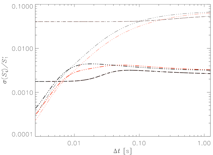
Figure 7: Same as Fig. 6, but for the case of a stepped modulator (with 8 states) consisting of a waveplate with $150^{\circ}$ retardance, identical to the one considered in Lites (1987). The same demodulation scheme of Lites (1987) was adopted for this calculation. These plots are for a dual-beam configuration with perfectly balanced beams. The gradients of the Stokes parameters are $g_{2}=g_{3}=S_{1}\,\mathrm{arcsec}^{-1}$ and $g_{1}=g_{4}=0$. The red curves (see on-line version of the figure) show the predicted cross-talk level neglecting terms of the form $g_{2}\,g_{3}$, which are missing in the treatment of Lites (1987); Judge et al. (2004).

Our formalism produces results that agree qualitatively with those found by Lites (1987) and Judge et al. (2004), although with some notable quantitative differences. Figure 7 shows the polarization cross-talk in a dual-beam configuration, calculated for a stepped modulator consisting of a rotating waveplate with $150^{\circ}$ retardance, identical to the one considered in the study by Lites (1987). The case considered in the figure corresponds to the presence of spatial gradients in $S_{2}$ and $S_{3}$ only. The red curves show the cross-talk that is derived by neglecting terms depending on $\bm{\nabla}S_{2}\cdot\bm{\nabla}S_{3}$, which are missing in the treatment by Lites (1987) and Judge et al. (2004) (see comment at the end of the next section).

7 Discussion

In this paper, we have approached the determination of seeing-induced cross-talk noise from a statistical point of view. Equations (10)–(12) and (14) and (15) form the basis of our derivation (see Sect. 3), so it is important to compare those results with previous work (Lites, 1987; Judge et al., 2004).

In the work of Lites (1987) and Judge et al. (2004), the “variances” there defined depend explicitly on the total observation time and the modulation frequency, through the integral of the product of the seeing power spectrum with a real function of frequency that depends implicitly on both (cf. Eq. [15] of Lites 1987, and points 1–5 of Sect. 2 of Judge et al. 2004). In our formalism, the total integration time does not appear explicitly because Eq. (12) represents the variance on a single measurement of $\mathscr{I}_{i}$. However, if a number $N$ of such measurements are made, and those measurements can be considered statistically uncorrelated, then the variance on the average signal $\bar{\mathscr{I}}_{i}$ is reduced by a factor $N$. In such case, for a fixed modulation frequency, but increasing the total observation time, we expect the same qualitative scaling of variance with the integration time as derived in previous work. Secondly, the dependence on the modulation frequency and the seeing power spectrum is also apparent within our formalism – already in the case of a single measurement – when we consider Eq. (9).

Incidentally, we note how the power spectrum of the seeing appears most naturally in our approach as the Fourier transform of the two-time correlation function of the seeing displacement vector (see Sect. 5), whereas in previous work it is identified instead with the modulus square of the Fourier transform of the seeing displacement. The correspondence between these two approaches to the definition of the power spectrum of a stationary random process is clearly described by Mandel & Wolf (1995).

The importance of the covariances $E([\mathscr{I}_{j}-\bar{\mathscr{I}}_{j}][\mathscr{I}_{k}-\bar{\mathscr{I}}_{k}])$ in typical cases has fundamental implications for the concept of polarimetric measurements. Through our analysis we are able to quantify the significance of seeing-induced correlations between measurements corresponding to different modulation steps, and how these correlations decay for decreasing modulation frequencies. Based on those results, it must be expected that seeing-induced correlations between different modulation states typically extend beyond the time interval of one modulation cycle. In other words, the Stokes vector measurements corresponding to different modulation cycles during an elemental observation are in general statistically correlated. Under this condition, we must expect that the variance of the average signal $\bar{\mathscr{I}}_{i}$ will obey the ordinary scaling law by the total number $N$ of cycles of the elemental observation only approximately. Formally, one should consider instead such elemental observation as a single measurement that is realized through the totality of the $N$ modulation cycles, and thus characterized by a corresponding $nN\times 4$ modulation matrix. The variance of this measurement can then be determined through the usual equations, adopting such extended definition of the modulation and demodulation matrices (see Sect. 6). A similar approach is taken also in the earlier work (Lites, 1987; Judge et al., 2004), where these correlations are made manifest by performing a spectral analysis of the demodulated signal over the entire time interval of the elemental observation.

Our formalism reveals however that, in the work of Lites (1987) and Judge et al. (2004), the covariance terms corresponding to contributions proportional to $\bm{\nabla}S_{i}\cdot\bm{\nabla}S_{j}$, with $i\neq j$ (see Eq. [5]), are not accounted for. In fact, Lites (1987) derives the variances as Eq. (12) of that paper directly from Eq. (11), which are explicitly of diagonal form. In other words, looking at our Eqs. (30) and (31), previous work has computed the seeing-induced noise always under the assumption that the gradient matrix $\tens{G}$ was diagonal. The additional off-diagonal components would arise in the development by Lites (1987) and Judge et al. (2004) when properly evaluating the expectation value of $(O_{r}-\bar{O}_{r})^{2}$ in the notation of Lites (1987). Equations (30) and (31) also clarify the vanishing of the cross-talk terms in the limit of large modulation frequencies ($\chi\Delta t\to 0$). Because all the integrals $\mathscr{T}_{|j-k|}(\Delta t)$ tend to the same value in such limit, the vector of the Stokes variances becomes simply proportional to the diagonal of the gradient matrix, $\tens{G}$.

Appendix A Beam imbalance introduced by a polarizing grating

We consider a beam of unpolarized light incident on a diffraction grating. Typically the diffraction efficiency of a grating is different in the $p$ and $s$ directions, so the diffracted beam consists of a mixture of two orthogonally polarized beams with generally different intensities $S_{\rm p}$ and $S_{\rm s}$. Let us consider the case in which these two beams get separated by a perfectly polarizing beam-splitter placed after the grating. The emerging beams will then have intensity $S_{\rm p}$ and $S_{\rm s}$, respectively.

Let us consider the combined signal of intensity $S$ so defined,

$$\bar{\kappa}S=\kappa_{\rm p}S_{\rm p}+\kappa_{\rm s}S_{\rm s}\;,\qquad\bar{\kappa}=\kappa_{\rm p}+\kappa_{\rm s}\;,$$

where $\kappa_{\rm p}$ and $\kappa_{\rm s}$ are the two gain factors applied to the detector to balance the two beams. The ratio $\kappa_{\rm p}/\kappa_{\rm s}$ then corresponds to the ratio of the two orthogonal efficiencies of the grating, $\epsilon_{\rm p}$ and $\epsilon_{\rm s}$, according to

$$\kappa_{\rm p}/\kappa_{\rm s}=\epsilon_{\rm s}/\epsilon_{\rm p}\;.$$ (A1)

The photon noise associated with the combined signal $S$ is given by

$$\sigma^{2}(S) = \left(\frac{\partial S}{\partial S_{\rm p}}\right)^{\!2}\sigma^{2}(S_{\rm p})+\left(\frac{\partial S}{\partial S_{\rm s}}\right)^{\!2}\sigma^{2}(S_{\rm s})$$

$$= \left(\frac{\kappa_{\rm p}}{\bar{\kappa}}\right)^{\!2}\sigma^{2}(S_{\rm p})+\left(\frac{\kappa_{\rm s}}{\bar{\kappa}}\right)^{\!2}\sigma^{2}(S_{\rm s})\;.$$

Correspondingly, the relative error is given by

$$\frac{\sigma^{2}(S)}{S^{2}}=\left(\frac{\kappa_{\rm p}S_{\rm p}}{\bar{\kappa}S}\right)^{\!2}\frac{\sigma^{2}(S_{\rm p})}{S_{\rm p}^{2}}+\left(\frac{\kappa_{\rm s}S_{\rm s}}{\bar{\kappa}S}\right)^{\!2}\frac{\sigma^{2}(S_{\rm s})}{S_{\rm s}^{2}}\;.$$

Evidently, for balanced beams

$$\kappa_{\rm p}S_{\rm p}=\kappa_{\rm s}S_{\rm s}=\textstyle{\frac{1}{2}}\bar{\kappa}S\;,$$ (A2)

and therefore

$$\frac{\sigma^{2}(S)}{S^{2}}=\frac{1}{4}\left[\frac{\sigma^{2}(S_{\rm p})}{S_{\rm p}^{2}}+\frac{\sigma^{2}(S_{\rm s})}{S_{\rm s}^{2}}\right]\;.$$ (A3)

If we express the signals in terms of photon flux, assuming Poisson’s statistics for the photon counts, and indicating with $r_{N}$ the read-out noise of the camera, we can rewrite Eq. (A3) as

$$\frac{\sigma^{2}(S)}{S^{2}} = \frac{1}{4}\left(\frac{N_{\rm p}+r_{N}^{2}}{N_{\rm p}^{2}}+\frac{N_{\rm s}+r_{N}^{2}}{N_{\rm s}^{2}}\right)$$ (A4)

$$= \frac{1}{4}\left(\frac{1}{N_{\rm p}}+\frac{1}{N_{\rm s}}\right)+\frac{r_{N}^{2}}{4}\left(\frac{1}{N_{\rm p}^{2}}+\frac{1}{N_{\rm s}^{2}}\right)\;.$$

If we indicate with $N_{\mathrm{in}}$ the photon count before the grating, evidently $N_{\rm p}=\frac{1}{2}\epsilon_{\rm p}N_{\mathrm{in}}$ and $N_{\rm s}=\frac{1}{2}\epsilon_{\rm s}N_{\mathrm{in}}$, so we find

$$\frac{\sigma^{2}(S)}{S^{2}} = \frac{1}{2N_{\mathrm{in}}}\,\frac{\epsilon_{\rm p}+\epsilon_{\rm s}}{\epsilon_{\rm p}\epsilon_{\rm s}}+\frac{r_{N}^{2}}{N_{\mathrm{in}}^{2}}\,\frac{\epsilon_{\rm p}^{2}+\epsilon_{\rm s}^{2}}{\epsilon_{\rm p}^{2}\epsilon_{\rm s}^{2}}$$ (A5)

$$= \frac{1}{N_{\mathrm{in}}}\,\frac{\bar{\epsilon}}{\epsilon_{\rm p}\epsilon_{\rm s}}+\frac{r_{N}^{2}}{N_{\mathrm{in}}^{2}}\,\frac{\epsilon_{\rm p}^{2}+\epsilon_{\rm s}^{2}}{\epsilon_{\rm p}^{2}\epsilon_{\rm s}^{2}}\;,$$

where we also introduced the grating’s average efficiency $\bar{\epsilon}=\frac{1}{2}(\epsilon_{\rm p}+\epsilon_{\rm s})$.

We note that the applicability of the above treatment in practical cases relies on the previous knowledge of the grating efficiencies, $\epsilon_{\rm p}$ and $\epsilon_{\rm s}$. These must be determined as a function of wavelength from flat-fielding, ideally using unpolarized radiation. If the incident beam is instead weakly polarized (as it is typically the case for sunlight flat-fields), the above treatment is still valid, but Eq. (A1) can only provide an approximate estimate of the appropriate gain factors, $\kappa_{\rm s}$ and $\kappa_{\rm p}$, if the measured efficiencies of the grating are adopted in that equation.

Appendix B Rotating modulator

We consider the case of a retarding device, which is continuously rotating with angular frequency $\Omega$, and which at $0^{\circ}$ position is described by the Mueller matrix

$$\bm{\mu}_{0}\equiv\begin{pmatrix}1&0&0&0\\ 0&\mu_{22}&\mu_{23}&\mu_{24}\\ 0&\mu_{32}&\mu_{33}&\mu_{34}\\ 0&\mu_{42}&\mu_{43}&\mu_{44}\end{pmatrix}\;,$$

where the following norm conditions must be satisfied,

$$\sum_{i}\mu_{ij}^{2}\leq 1\;,\qquad\sum_{j}\mu_{ij}^{2}\leq 1\;.$$

We note that a full modulation cycle corresponds to only half rotation of the modulator, because of the characteristic $180^{\circ}$-periodicity of polarization modulation.

In order to determine the cross-talk terms (40) for such a device, we need to compute the Fourier transforms of the functions (see Eq. [39])

$$Z_{jk}(\xi)\equiv\Pi_{\Delta t}(\xi)\,m_{j}(\xi+t_{k})\;,\qquad j=1,\dots,4\;,\quad k=1,\ldots,n\;,$$

where $n$ is the number of modulation states (camera exposures) in the modulation cycle. These Fourier transforms are given by the following expressions,

$$\tilde{Z}_{1k}(\omega) = \Delta t\;\textrm{sinc}(\omega\Delta t/2)\;,$$

$$\tilde{Z}_{2k}(\omega) = \frac{1}{2}\,(\mu_{22}+\mu_{33})\,\Delta t\;\textrm{sinc}(\omega\Delta t/2)$$

$$\kern 14.22636pt+\frac{1}{4}\,[\mu_{22}-\mu_{33}+\mathrm{i}(\mu_{23}+\mu_{32})]\,\mathrm{e}^{4\mathrm{i}[\Omega t_{1}+\pi(k-1)/n]}\,\Delta t\;\textrm{sinc}\bigl{(}[\omega-4\Omega]\Delta t/2\bigr{)}$$

$$\kern 14.22636pt+\frac{1}{4}\,[\mu_{22}-\mu_{33}-\mathrm{i}(\mu_{23}+\mu_{32})]\,\mathrm{e}^{-4\mathrm{i}[\Omega t_{1}+\pi(k-1)/n]}\,\Delta t\;\textrm{sinc}\bigl{(}[\omega+4\Omega]\Delta t/2\bigr{)}\;,$$

$$\tilde{Z}_{3k}(\omega) = \frac{1}{2}\,(\mu_{23}-\mu_{32})\,\Delta t\;\textrm{sinc}(\omega\Delta t/2)$$

$$\kern 14.22636pt-\frac{\mathrm{i}}{4}\,[\mu_{22}-\mu_{33}+\mathrm{i}(\mu_{23}+\mu_{32})]\,\mathrm{e}^{4\mathrm{i}[\Omega t_{1}+\pi(k-1)/n]}\,\Delta t\;\textrm{sinc}\bigl{(}[\omega-4\Omega]\Delta t/2\bigr{)}$$

$$\kern 14.22636pt+\frac{\mathrm{i}}{4}\,[\mu_{22}-\mu_{33}-\mathrm{i}(\mu_{23}+\mu_{32})]\,\mathrm{e}^{-4\mathrm{i}[\Omega t_{1}+\pi(k-1)/n]}\,\Delta t\;\textrm{sinc}\bigl{(}[\omega+4\Omega]\Delta t/2\bigr{)}\;,$$

$$\tilde{Z}_{4k}(\omega) = \frac{1}{2}\,(\mu_{24}+\mathrm{i}\mu_{34})\mathrm{e}^{2\mathrm{i}[\Omega t_{1}+\pi(k-1)/n]}\,\Delta t\;\textrm{sinc}\bigl{(}[\omega-2\Omega]\Delta t/2\bigr{)}$$

$$+ \frac{1}{2}\,(\mu_{24}-\mathrm{i}\mu_{34})\mathrm{e}^{-2\mathrm{i}[\Omega t_{1}+\pi(k-1)/n]}\,\Delta t\;\textrm{sinc}\bigl{(}[\omega+2\Omega]\Delta t/2\bigr{)}\;,$$

where $\Delta t$ is the exposure time for each modulation state, and $t_{1}$ is the time at which the modulator is found in the $0^{\circ}$ position.

Figure 1: Two-time correlations of the normalized amplitudes of the seeing displacement vector, $\mathscr{T}_{|j-k|}(\Delta t)$, plotted against the normalized exposure time, $\chi\Delta t$, for various values of $|j-k|$: 0 (variance; thick continuous line); 1 (first neighbor; dotted line); 2 (second neighbor; dashed line); 3 (third neighbor; dot-dashed line). For this calculation, we used the expression (29) for the auto-correlation function $\Gamma(t)$, and a duty cycle $r=1$ for the camera.

Figure 2: Power spectra of a seeing-like random process. The thin curve represents the normalized power spectrum corresponding to the auto-correlation function (29). The thick curve shows a simple analytic modification of this spectrum, presenting characteristics similar to those produced by the action of adaptive optics.

Figure 3: Normalized auto-correlation function corresponding to the two power spectra of Fig. 2. The thin curve corresponds to Eq. (29) [after normalization by $\Gamma(0)$], whereas the thick curve corresponds to the AO-corrected spectrum. Note the significant reduction of the time interval within which an efficient suppression of the auto-correlation of the seeing is attained in the presence of AO correction.

Figure 4: Same as Fig. 1, but assuming the AO-corrected auto-correlation function shown in Fig. 3. Note the significant damping of the covariances for a given value of $\chi\Delta t$, compared to the case of uncorrected seeing. As for Fig. 1, a camera duty cycle $r=1$ was assumed for this calculation.

Figure 5: Plots of the Stokes errors of Eq. (40) normalized to the incoming intensity, as a function of the modulation frequency. The case shown corresponds to the balanced scheme of Eq. (35) in single-beam configuration, with non-zero gradients of the Stokes parameters, such that $g_{1}=g_{4}=S_{1}\,\mathrm{arcsec}^{-1}$ and $g_{2}=g_{3}=0.1\,g_{1}$: continuous curve, $\sigma(S_{1}^{\prime})$; dashed curve, $\sigma(S_{2}^{\prime})$; dash-dotted curve, $\sigma(S_{3}^{\prime})$; dash-triple-dotted curve, $\sigma(S_{4}^{\prime})$. These plots were calculated for a total modulation time $T=10\,\mathrm{s}$, assuming a camera duty cycle $r=1$. The thin curves are for an observed power spectrum of the seeing, while the thick curves show the effects of AO correction (power spectra courtesy of T. Rimmele).

Figure 6: Same as Fig. 5, but for the dual-beam configuration with perfectly balanced beams.

References

- Asensio Ramos & Collados (2008) Asensio Ramos, A., & Collados, M. 2008, Appl. Opt., 47, 2541
- Born & Wolf (1965) Born, M., & Wolf, E. 1965, Principles of Optics, 3rd ed. (Pergamon: Oxford)
- Collados (2008) Collados, M. 2008, SPIE, 7012, 17
- Draper & Smith (1966) Draper, N. R., & Smith, H. 1966, Applied Regression Analysis (Wiley: New York)
- Fried (1965) Fried, D. L. 1965, J. Opt. Soc. Am., 55, 1427
- Goodman (1996) Goodman, J. W. 1996, Introduction to Fourier Optics, 2nd ed. (McGraw-Hill: New York)
- Judge et al. (2004) Judge, P. G., Elmore, D. F., Lites, B. W., Keller, C. U., Rimmele, T. 2004, Appl. Opt., 43, 3817
- Lites (1987) Lites, B. W. 1987, Appl. Opt., 26, 3838
- Mandel & Wolf (1995) Mandel, L., & Wolf, E. 1995, Optical Coherence and Quantum Optics (Cambridge: Cambridge)
- Martínex Pillet et al. (2011) Martínez Pillet, V., del Toro Iniesta, J. C., Álvarez-Herrero, A., Domingo, V., Bonet, J. A., et al. 2011, Solar Phys., 268, 57
- Noll (1976) Noll, R. J. 1976, J. Opt. Soc. Am., 66, 207
- Rimmele et al. (2008) Rimmele, T., & the ATST Team 2008, Adv. Sp. Res., 42, 78
- Scherrer et al. (2012) Scherrer, P. H., Schou, J., Bush, R. I., Kosovichev, A. G., Bogart, R. S. 2012, Solar Phys., 275, 207
- Shimizu et al. (2011) Shimizu, T., Tsuneta, S., Hara, H., Ichimoto, K., Kusano, K., et al. 2011, SPIE, 8148, 10
- Tatarski (1961) Tatarski, V. I. 1961, Wave Propagation in a Turbulent Medium (Dover: New York)
- del Toro Iniesta & Collados (2000) del Toro Iniesta, J. C., & Collados, M. 2000, Appl. Opt., 39, 1637
- Tsuneta et al. (2008) Tsuneta, S., Ichimoto, K., Katsukawa, Y., Nagata, S., Otsubo, M., et al. 2008, Solar Phys., 249, 167
- Van Cittert (1934) Van Cittert, P. H. 1934, Phy., 1, 201
- Zernike (1938) Zernike, F. 1938, Phy., 5, 785