Formation of singularities in solutions to ideal hydrodynamics of freely cooling inelastic gases

Abstract

We consider solutions to the hyperbolic system of equations of ideal granular hydrodynamics with conserved mass, total energy and finite momentum of inertia and prove that these solutions generically lose the initial smoothness within a finite time in any space dimension $n$ for the adiabatic index $\gamma\leq 1+\frac{2}{n}.$ Further, in the one-dimensional case we introduce a solution depending only on the spatial coordinate outside of a ball containing the origin and prove that this solution under rather general assumptions on initial data cannot be global in time too. Then we construct an exact axially symmetric solution with separable time and space variables having a strong singularity in the density component beginning from the initial moment of time, whereas other components of solution are initially continuous.

1 Introduction

The motion of the dilute gas where the characteristic hydrodynamic length scale of the flow is sufficiently large and the viscous and heat conduction terms can be neglected is governed by the systems of equations of ideal granular hydrodynamics [1].

This system is given in ${\mathbb{R}}\times{\mathbb{R}}^{n},\,n\geq 1,$ and has the following form:

$$\partial_{t}\rho+{\rm div}_{x}(\rho u)=0,$$ (1.1)

$$\partial_{t}(\rho u)+{\rm Div}_{x}(\rho u\otimes u)=-\nabla_{x}p,$$ (1.2)

$$\partial_{t}T+(u,\nabla_{x}T)+(\gamma-1)T{\rm div}_{x}u=-\Lambda\rho T^{3/2},$$ (1.3)

where $\rho$ is the gas density, $u=(u_{1},...,u_{n})$ is the velocity, $T$ is the temperature, $p=\rho T$ is the pressure, and $\gamma$ is the adiabatic index $(1<\gamma\leq 1+\frac{2}{n}),$ $\Lambda=const>0.$ we denote ${\rm Div}_{x}$ and ${\rm div}_{x}$ the divergency of tensor and vector, respectively, with respect to the space variables. The only difference between equations (1.1)–(1.3) and the standard ideal gas dynamic equations (where the elastic colliding of particles is supposed) is the presence of the inelastic energy loss term $-\Lambda\rho T^{3/2}$ in (1.3).

The granular gases are now popular subject of experimental, numerical and theoretical investigation (e.g. [1], [7], [4] and references therein). In contrast to ordinary molecular gases, granular gases cool spontaneously because of the inelastic collisions between the particles. The inelasticity of the collisions generally causes the granular gas to form dense clusters. The formation of complex structure of clusters has been investigated by means of molecular dynamics simulations and hydrodynamic simulations.

The Navier-Stokes granular hydrodynamics is the natural language for a theoretical description of granular macroscopic flows. A characteristic feature of time-dependent solutions of the continuum equations is a formation of finite-time singularities: the density blowup signals the formation of close-packed clusters.

System (1.1) – (1.3) can be written in a hyperbolic symmetric form in variables $\,\rho,\,u,K=p\rho^{-\gamma}\,$ and therefore the Cauchy problem

$$\rho,u,p\rho^{-\gamma}\big{|}_{t=0}\in H^{m}({\mathbb{R}}^{n}),\,m\geq 1+\left[\frac{n}{2}\right].$$

has a solution as smooth as initial data at least for small $t>0$ [6].

We will call the solution to (1.1) – (1.3) classical if $\rho>0,p>0$ and the components of solution belongs to $C^{1}([0,T),H^{m}({\mathbb{R}}^{n})),\,T\leq\infty.$

System (1.1) – (1.3) has no constant solution except the trivial one $(p\equiv 0),$ therefore the solution with the components highly decreasing as $|x|\to\infty$ can be considered as a natural perturbation if this steady state in the case of the mass conservation.

Let us note that there exists a solution (the homogeneous cooling state) with constant $\rho,u$ and $p\neq 0$. In this case the temperature $T=T(t)=(\frac{\Lambda\rho_{0}t}{2}+T(0)^{-1})^{-2},$ where $T(0)$ is the initial value of temperature (the Haff’s law). Another trivial solution is $u=p=T\equiv 0,\,\rho(t,x)=\rho_{0}(x)$.

We introduce the following integrals: the total mass

$$M(t)=\int\limits_{{\mathbb{R}}^{n}}\rho\,dx,$$

the momentum

$$P(t)=\int\limits_{{\mathbb{R}}^{n}}\rho u\,dx,$$

and the total energy

$$\mathcal{E}(t)=\int\limits_{{\mathbb{R}}^{n}}\left(\frac{1}{2}\rho|u|^{2}+\rho T\right)\,dx\,=E_{k}(t)+E_{i}(t).$$

Here $E_{k}(t)$ and $E_{i}(t)$ are the kinetic and internal components of energy, respectively. Let us introduce also the functionals

$$G(t)=\frac{1}{2}\int\limits_{{\mathbb{R}}^{n}}\rho(t,x)|{x}|^{2}\,dx,\qquad F(t)=\int\limits_{{\mathbb{R}}^{n}}({u},{x})\rho\,dx,$$

where the first one is the momentum of inertia.

We consider below the solutions to (1.1) – (1.3) such that the integrals $m,P,E$ and $G$ converge and call them solutions with finite momentum of inertia  (FMI). It is easy to verify that for this class of solutions $M(t)=M=const,\,P(t)=P=const,$

$$\mathcal{E}^{\prime}(t)=-\frac{\Lambda}{\gamma-1}\,\int\limits_{{\mathbb{R}}^{n}}\rho^{1/2}\,p^{3/2}\,dx.$$ (1.4)

The latter equation expresses the inelastic energy loss per collision.

Further we consider a function $K=p\,\rho^{-\gamma},$ where $\ln K$ can be interpreted as the usual hydrodynamic entropy. System (1.1) – (1.3) result

$$\frac{dK}{dt}=-\Lambda\,K^{\frac{3}{2}}\,\rho^{\frac{\gamma+1}{2}}\leq 0,$$

therefore

$$K(t,x)\leq K_{+}=\sup\limits_{x\in{\mathbb{R}}^{n}}K(0,x).$$ (5)

2 Main theorem: nonexistence of global smooth solutions

Theorem 1

Let $P\neq 0$ and $M$ be sufficiently small. Then there exists no global in time classical FMI solution to the Cauchy problem for (1.1) – (1.3).

To prove the theorem we need to get firstly certain estimates of energy.

Lemma 1

For the classical FMI solutions to (1.1) – (1.3) the following estimates hold:

$$E_{k}(t)\geq\frac{P^{2}}{2M}=const,$$ (1)

$$\mathcal{E}^{\prime}(t)\leq-\Lambda C_{1}E_{i}^{\frac{3\gamma-1}{2(\gamma-1)}}(t),$$ (2)

where $C_{1}=K_{+}^{-\frac{1}{\gamma-1}}\,(\gamma-1)^{\frac{3\gamma-1}{2(\gamma-1)}}\,M^{-\frac{\gamma+1}{2(\gamma-1)}}.$

Proof. Inequality (1) follows immediately from the Hölder inequality. To prove (2) we firstly use the Jensen inequality as follows:

$$\left(\frac{\int\limits_{{\mathbb{R}}^{n}}\,p\,dx}{M}\right)^{\frac{3\gamma-1}{2(\gamma-1)}}=\left(\frac{\int\limits_{{\mathbb{R}}^{n}}\,K\rho\rho^{\gamma-1}\,dx}{M}\right)^{\frac{3\gamma-1}{2(\gamma-1)}}$$

$$\leq\frac{\int\limits_{{\mathbb{R}}^{n}}\,\rho K^{\frac{3\gamma-1}{2(\gamma-1)}}\,\rho^{\frac{3\gamma-1}{2}}\,dx}{M}\leq\frac{\int\limits_{{\mathbb{R}}^{n}}\,\rho^{1/2}\,p^{3/2}\,K^{\frac{1}{\gamma-1}}\,dx}{M}\leq\frac{K_{+}^{\frac{1}{\gamma-1}}}{M}{\int\limits_{{\mathbb{R}}^{n}}\,\rho^{1/2}\,p^{3/2}\,dx}.$$ (3)

Together with (1.4) inequality (3) gives (2). $\square$ The following lemmas establish the properties of the momentum of inertia. Acting as in [2] we get

Lemma 2

For classical FMI solutions to (1.1) – (1.3) the equalities

$$G^{\prime}(t)=F(t),$$ (4)

$$F^{\prime}(t)=2E_{k}(t)+n(\gamma-1)E_{i}(t).$$ (5)

take place.

Proof. The lemma can be proved by direct calculation using the general Stokes formula. $\square$ Then we get two-sided estimates of $G(t).$

Lemma 3

If $\gamma\leq 1+\frac{2}{n},$ then for the classical FMI solutions to (1.1) – (1.3) the estimates

$$\frac{P^{2}}{2M}t^{2}+F(0)t+G(0)\leq G(t)\leq\mathcal{E}(0)t^{2}+F(0)t+G(0)$$ (6)

hold.

Proof. First of all (6), (2) result

$$G^{\prime\prime}(t)=2E_{k}(t)+n(\gamma-1)E_{i}(t)=2\mathcal{E}(t)-(2-n(\gamma-1))E_{i}(t).$$

Therefore together with (1) we have

$$\frac{P^{2}}{M}\,\leq\,G^{\prime\prime}(t)\leq\,2\mathcal{E}(0),$$ (7)

after integration this gives (6). $\square$ Now we get an upper estimate of $E_{i}(t).$

Lemma 4

If $\gamma\leq 1+\frac{2}{n}$ and $P\neq 0,$ then for the classical FMI solutions the following estimate is true:

$$E_{i}(t)\leq\frac{C_{2}}{G^{n(\gamma-1)/2}},$$ (8)

where $C_{2}=\frac{(4G(t)\mathcal{E}(t)-F^{2}(t))G^{(\gamma-1)n/2}(0)}{4}.$

Proof. The method of obtaining the upper estimate of $E_{i}(t)$ is similar to [2]. Namely, let us consider the function $Q(t)=4G(t)\mathcal{E}(t)-F^{2}(t).$ The Hölder inequality gives $F^{2}\leq 4G(t)E_{k}(t),$ therefore $\mathcal{E}(t)=E_{k}(t)+E_{i}(t)\geq E_{i}(t)+\frac{F^{2}(t)}{4G(t)}$ and

$$E_{i}(t)\leq\frac{Q(t)}{4G(t)}.$$ (9)

We notice also that $Q(t)>0$ provided the pressure does not equal to zero identically. Then taking into account (4), (5) and (2) we have

$$Q^{\prime}(t)=4G^{\prime}(t)\mathcal{E}(t)-2G^{\prime}(t)G^{\prime\prime}(t)+4G(t)\mathcal{E}^{\prime}(t)$$

$$=2(2-n(\gamma-1))\,G^{\prime}(t)E_{i}(t)+4G(t)\mathcal{E}^{\prime}(t).$$ (10)

Further, one can see from (7) that $G^{\prime}(t)>0$ beginning from a positive $t_{0}$ for all initial data. Thus, for $\gamma\leq 1+\frac{2}{n}$ we have from (9), (2)

$$\frac{Q^{\prime}(t)}{Q(t)}\leq\frac{2-n(\gamma-1)}{2}\,\frac{G^{\prime}(t)}{G(t)}.$$ (11)

Then (9) and (11) give

$$E_{i}(t)\leq\frac{C_{2}}{G^{(\gamma-1)n/2}(t)},\quad C_{2}=\frac{Q(0)G^{(\gamma-1)n/2}(0)}{4}.$$

The proof is over. $\square$

Remark 1

Inequalities (1) and (2) result

$$\mathcal{E}^{\prime}(t)\leq-\Lambda\,C_{1}\,\left(\mathcal{E}(t)-\frac{P^{2}}{2M}\right)^{\frac{3\gamma-1}{2(\gamma-1)}}.$$

Integrating this inequality we the following upper estimate of $E_{i}(t):$

$$E_{i}(t)\leq(c_{1}\,t+c_{2})^{-\frac{2(\gamma-1)}{\gamma+1}},$$

where $c_{1}=\frac{\Lambda C_{1}(\gamma+1)}{\gamma-1}$ and $c_{2}=(E(0)-P^{2}/(2M))^{\frac{2(\gamma-1)}{\gamma+1}}$ are positive constants. However, for $\gamma\leq 1+\frac{2}{n}$ this estimate is less exact than (8) and is not enough for our proof.

The next step is a lower estimate of $E_{i}(t).$

Lemma 5

Let $P\neq 0.$ Then for the classical FMI solutions the estimate

$$E_{i}(t)\geq\frac{C_{3}}{G^{(\gamma-1)n/2}(t)},$$ (12)

holds with a positive constant

$$C_{3}=\frac{1}{2^{(\gamma-1)n/2}\,K_{+}^{(\gamma-1)(1+n/2)}\,(\gamma-1)}\,{C_{\gamma,n}^{-\frac{\gamma(n+2)-2}{2}}}\,(C_{6}(\gamma))^{\frac{(\gamma-1)\gamma(n+2)-2}{4\gamma-1}},$$

the value of $C_{6}$ is written in (18).

Proof. The proof is based on the inequality

$$\|f\|_{L^{1}({\mathbb{R}}^{n};\,dx)}\,\leq\,C_{\gamma,n}\,\|f\|^{\frac{2\gamma}{(n+2)\gamma-n}}_{L^{\gamma}({\mathbb{R}}^{n};\,dx)}\,\|f\|^{\frac{n(\gamma-1)}{(n+2)\gamma-n}}_{L^{1}({\mathbb{R}}^{n};\,|x|^{2}\,dx)},$$

$$C_{\gamma,n}=\left(\frac{2\gamma}{n(\gamma-1)}\right)^{\frac{n(\gamma-1)}{(n+2)\gamma-n}}+\left(\frac{2\gamma}{n(\gamma-1)}\right)^{\frac{-2\gamma}{(n+2)\gamma-n}},$$

established in [2]. Namely, we have for $f=K\rho$

$$E_{i}(t)=\frac{1}{\gamma-1}\,\int\limits_{{\mathbb{R}}^{n}}\,\frac{p}{\rho^{\gamma}}\,\frac{(K\rho)^{\gamma}}{K^{\gamma}}\,dx\geq\frac{1}{K_{+}^{\gamma-1}\,(\gamma-1)}\,\int\limits_{{\mathbb{R}}^{n}}\,(K\rho)^{\gamma}\,dx\,$$

$$\geq\,\frac{1}{K_{+}^{\gamma-1}\,(\gamma-1)}\,\frac{\left(C^{-1}_{\gamma,n}\,\int\limits_{{\mathbb{R}}^{n}}\,K\rho\,dx\right)^{\frac{\gamma(n+2)-2}{2}}}{\left(\int\limits_{{\mathbb{R}}^{n}}\,K\rho|x|^{2}\,dx\right)^{\frac{n(\gamma-1)}{2}}}$$

$$\geq\,\frac{1}{2^{(\gamma-1)n/2}\,K_{+}^{(\gamma-1)(1+n/2)}\,(\gamma-1)}\,\frac{\left(C^{-1}_{\gamma,n}\,S(t)\right)^{\frac{\gamma(n+2)-2}{2}}}{(G(t))^{\frac{n(\gamma-1)}{2}}},$$ (13)

where we denoted $S(t)=\int\limits_{{\mathbb{R}}^{n}}\,K\rho\,dx.$ Further, from (1.1) and (1) we have

$$\partial_{t}(K\rho)+{\rm div}_{x}(K\rho u)=-\Lambda K^{\frac{3}{2}}\rho^{\frac{\gamma+3}{2}},$$

therefore

$$S^{\prime}(t)=-\Lambda\,\int\limits_{{\mathbb{R}}^{n}}\,K^{\frac{3}{2}}\,\rho^{\frac{\gamma+3}{2}}\,dx.$$ (14)

From the Jensen inequality we get

$$\int\limits_{{\mathbb{R}}^{n}}\,K^{\frac{3}{2}}\,\rho^{\frac{\gamma+3}{2}}\,dx\leq\frac{K_{+}^{\frac{3}{2}}\,M}{S(t)}\int\limits_{{\mathbb{R}}^{n}}\,K\,\rho\,\rho^{\frac{\gamma+1}{2}}\,dx\leq K_{+}^{\frac{3}{2}}M\,\left(\frac{\int\limits_{{\mathbb{R}}^{n}}\,K\,\rho^{\gamma}\,dx}{S(t)}\right)^{\frac{1+\gamma}{2(\gamma-1)}}$$

$$=C_{4}\,\left(\frac{E_{i}(t)}{S(t)}\right)^{\frac{1+\gamma}{2(\gamma-1)}},$$ (15)

where $C_{4}=K_{+}^{\frac{3}{2}}M(\gamma-1)^{\frac{1+\gamma}{2(\gamma-1)}}.$ Further, from (8), (14), (15) we obtain

$$S^{\frac{1+\gamma}{2(\gamma-1)}}(t)\,S^{\prime}(t)\geq-\Lambda C_{4}\,C_{2}^{\frac{\gamma+1}{2(\gamma-1)}}\,(G(t))^{-\frac{n(\gamma+1)}{4}}.$$ (16)

Now we take into account the lower estimate in (6) together with the fact that beginning from a certain $t_{0}$ the value of $F(t)$ becomes positive if $P\neq 0$ (see (1), (5)) and integrate (16). Thus for $t\geq t_{0}$ we get in the case $\gamma<3$

$$S(t)\geq\left(S(t_{0})^{\frac{\gamma-3}{2(\gamma-1)}}+\Lambda\frac{4(\gamma-1)}{(3-\gamma)(n(\gamma-1)-2)}\,C_{5}^{1-\frac{n(\gamma+1)}{2}}\right)^{\frac{2(\gamma-1)}{\gamma-3}},$$ (17)

where $C_{5}=M\,(F(t_{0}))^{-\frac{n(\gamma+1)}{2}}\,P^{-2},$ and for $\gamma=3$  $(n=1)$

$$S(t)\geq S(t_{0})\,\exp\left(\frac{2\Lambda}{C_{5}}\right).$$ (18)

We denote the constant in the right-hand side of (17), (18) by $C_{6}(\gamma).$ It is easy to see that for sufficiently large $t$ the value of $S(t)$ is separated from zero. Thus, from (13), (17), (18) we obtain (12). $\square$

Proof of Theorem 1

Taking into account (2), (12) and the right-hand side of (6) we get

$$\mathcal{E}^{\prime}(t)\leq-\Lambda C_{1}\,C_{3}^{\frac{3\gamma-1}{2(\gamma-1)}}\,(G(t))^{-\frac{n(3\gamma-1)}{4}}$$ (19)

$$\leq-\Lambda C_{1}\,C_{3}^{\frac{3\gamma-1}{2(\gamma-1)}}\,(\mathcal{E}(0)t^{2}+F(0)t+G(0))^{-\frac{n(3\gamma-1)}{4}}.$$

As follows from (1), (4) beginning from $t_{0}>0$ the value of $F(t)$ becomes positive. Integrating (19) we obtain for $t>t_{0}$

$$\mathcal{E}(t)\leq\mathcal{E}(t_{0})-\Lambda\,C_{1}\,C_{3}^{\frac{3\gamma-1}{2(\gamma-1)}}\,\frac{2^{n(3\gamma-1)/2}(F(t_{0}))^{-n(3\gamma-1)/2+1}(\mathcal{E}(0))^{n(\gamma-1)/4-1}}{n(3\gamma-1)-2}+\lambda(t),$$

where $\lambda(t)=\Or(t^{-n(3\gamma-1)/2+1}),\,t\to\infty.$ Since $C_{3}$ tends to a positive constant as $M\to 0$ and $C_{1}$ contains $M$ in a negative degree (see the statements of Lemmas 1 and 5, then choosing $M$ sufficiently small, we can always get a contradiction with inequality (1). This prove the theorem. $\square$

Remark 2

Main idea of this paper can be found in [8], where it was proved nonexistence of global smooth solutions to the compressible Navier-Stokes equations. For the freely cooling gas, it would be possible to add viscous terms (with constant viscosity coefficients) to apply the same technique and obtain the analogous nonexistence result.

3 One-dimensional case

As it was noticed system (1.1) – (1.3) has no constant solution except of the trivial one $p\equiv 0.$ However, it is possible to construct the nontrivial steady state solution $\bar{\rho}(0,x),\bar{v}(0,x),\bar{p}(0,x)$ for the regions $|x|>R(t)>0.$ For $|x|\leq R(0)$ we chose the functions $\,\rho(0,x),\,v(0,x),\,p(0,x)\,$ arbitrarily to get initial data, smooth on the whole real axis. We are going to show that such solution necessarily loses its initial smoothness.

3.1 Automodel solution

Let us find a solution that depends on the automodel variable $\xi=x-at,\,a=const.$ The continuity equation (1.1) gives the connection between the velocity and density as follows:

$$u(\xi)=\frac{c_{1}}{\rho(\xi)}+a,\,c_{1}=const\neq 0.$$ (1)

Equation (1.2) and (1) results

$$c_{1}u(\xi)+p(\xi)=c_{2},\,c_{2}=const.$$ (2)

From (1) and (2) we have $c_{1}^{2}+\rho p=\rho(c_{2}-ac_{1})$, therefore $c_{2}-ac_{1}>0$. Further, we substitute the functions $u$ and $p,$ found from (3.1) and (3.2) and expressed through $\rho,$ in the equation

$$\partial_{t}p+u\partial_{x}p+\gamma p\partial_{x}u=-\Lambda\rho^{2}p^{3/2},$$

which is a corollary of (1.1), (1.3) and the state equation $p=\rho T$. Thus we get an ordinary differential equation

$$\rho^{\prime}(\xi)=\,-\,\frac{\Lambda}{c_{1}}\,\frac{\rho^{2}(\xi)\,((c_{2}-ac_{1})\rho(\xi)-c_{1}^{2})^{3/2}}{c_{1}^{2}(\gamma+1)-\gamma(c_{2}-ac_{1})\rho(\xi)},$$

or

$$z^{\prime}(\xi)=-\frac{\Lambda}{c_{1}(c_{2}-ac_{1})}\,\frac{z^{3/2}(\xi)(z(\xi)+c_{1}^{2})^{2}}{c_{1}^{2}-\gamma z(\xi)},$$ (3)

where $z=(c_{2}-ac_{1})\rho-c_{1}^{2}.$ The case $c_{2}-ac_{1}=0$ that seems simpler corresponds to a negative pressure and we do not consider it. Equation (3) has a solution

$$\xi=f(z):=\frac{c_{2}-ac_{1}}{c_{1}\,\Lambda}\left(\frac{(\gamma+3)\,\arctan\frac{\sqrt{z}}{c_{1}}}{c_{1}}\,+\,\,\frac{(\gamma+1)\sqrt{z}}{z+c^{2}_{1}}\,+\,\frac{2}{\sqrt{z}}\right)\,+\,c_{3},$$ (4)

$\,c_{3}=const$. One can see from (3) that if $z(\xi_{0})\leq z_{*}=\frac{c_{1}^{2}}{\gamma}$, then there exists a branch of solution (4) defined on the semi-axis $(\xi_{0},+\infty)$ for positive $c_{1}\,$ where the function $z(\xi)$ decrease monotonically from the value $z(\xi_{0})$ to zero. For negative $c_{1}\,$ this branch is defined on the semi-axis $(-\infty,\xi_{0}),$ where the function $z(\xi)$ increase monotonically from zero to $z(\xi_{0})$.

3.2 ”Finally steady state” and its smooth compact perturbation

Let us consider a stationary solution for $a=0,$ $\xi=x$, choose a point $x_{0}\geq 0$, a constant $c_{1}=u(x_{+})\rho(x_{+})>0$, and construct on the semi-axis $x>x_{+}$ a solution $z_{+}(x)$. Analogously for the semi-axis $x\leq x_{-}$ we choose $c_{1}=u(x_{-})\rho(x_{-})<0$ and construct a solution $z_{-}(x).$ Thus, outside of the segment $[x_{-},x_{+}]$ we define a solution

$$\bar{z}(x)=\left\{\begin{array}[]{ll}z_{-}(x),&\quad x\in(-\infty,\,x_{-}),\\ z_{+}(x),&\quad x\in(x_{+},+\infty).\end{array}\right.$$

For the sake of simplicity we set $x_{-}=-x_{+}$, $c_{1}=-k$ for $z_{-}(x)$ and $c_{1}=k$ for $z_{+}(x)$, where $k=const>0$. In their turn, the density, pressure and velocity can be found as

¯ρ

=¯z+k2c2, ¯p=c_2-k2¯ρ, ¯u=k sign x  ¯ρ. It is very attractive to choose $x_{+}=x_{-}=0$ and to construct a piecewise continuous solution like a solution of a ”Riemmann problem” with non-constant left and right states. Nevertheless, it can be readily shown that the Hugoniot conditions do not hold on the jump. Indeed, the components $\bar{\rho}$ and $\bar{p}$ are continuous at the point $x=0,$ having a jump in derivative, however, the velocity itself has a jump $[\bar{u}]=\frac{2k}{\bar{\rho}(0)}\geq\frac{2\gamma c_{2}}{k(\gamma+1)}$ (see Figs.1 – 3). The value of $[\bar{u}]$ tends to zero as $k\to\infty,$ however the Hugoniot condition $[\bar{\rho}\bar{u}]=0$ does not implement in the origin $x=0.$ Of course, we can choose $c_{1}$ such that the density and pressure have jumps in the origin and consider $a\neq 0$, nevertheless the careful analysis shows that the Hugoniot conditions do not hold anyway.

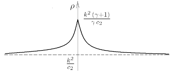
Figure 1: The density

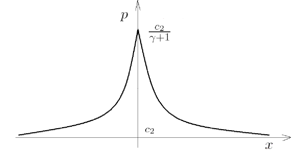
Figure 2: The pressure

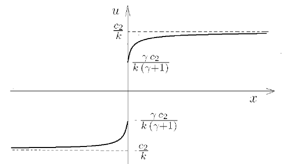
Figure 3: The velocity

Therefore we choose $R(0)>x_{+},$ and define smooth initial data such that for $|x|>R(0)$ they coincide with $\bar{\rho}(x),\,\bar{u}(x),\,\bar{p}(x)$ and on the segment $|x|\leq R(0)$ they are arbitrary smooth functions $\,\rho(0,x)>0,\,p(0,x)>0,\,u(0,x).$ We will call this type of initial data the compact perturbation of nontrivial finally steady state. Let us note that for $k=0$ we get the trivial zero-state solution.

3.3 Breakdown of the compact perturbation of the nontrivial ”finally steady state”

Let us denote the perturbed region by $B(t):=\{x\big{|}\,|x|\leq R(t)\},$ and consider the analogs of functionals used in the previous section:

$$\tilde{G}(t)=\frac{1}{2}\,\int\limits_{B(t)}\,\rho(t,x)|x|^{2}\,dx,\qquad\tilde{F}(t)=\int\limits_{B(t)}\,\rho(t,x)(u(t,x),x)\,dx,$$

$$\tilde{E}_{k}(t)=\frac{1}{2}\,\int\limits_{B(t)}\,\rho(t,x)|u(t,x)|^{2}\,dx,\qquad\tilde{M}(t)=\int\limits_{B(t)}\,\rho(t,x)\,dx.$$

$$\tilde{P}(t)=\,\int\limits_{B(t)}\,\rho(t,x)\,u(t,x)\,dx,\quad\tilde{S}(t)=\,\int\limits_{B(t)}\,K(t,x)\rho(t,x)\,dx.$$

The following theorem holds:

Theorem 2

Let $\tilde{P}^{2}(0)>\frac{8\tilde{M}c_{2}}{k},\,n=1.$ Then there exists no globally in $t$ smooth perturbation of the nontrivial steady state for system (1.1)– (1.3).

Proof. First of all we note that system (1.1)– (1.3) is hyperbolic and therefore the speed of boundary of the perturbations is equals to $|\bar{u}|+V_{s},$ where $V_{s}=\sqrt{\bar{p}_{\bar{\rho}}},$ the sound speed. As follows from (3.2),

$$V_{s}=\frac{k}{\bar{\rho}}\leq\frac{c_{2}}{k}:=\sigma,$$ (5)

where we use the estimate $\bar{\rho}\geq\frac{k^{2}}{c_{2}}.$ Then we have

$$\tilde{F}^{\prime}(t)=2\tilde{E}_{k}+\int\limits_{B(t)}\,(p(t,x)-\bar{p}(t,R(t)))\,dx,$$ (6)

$$\tilde{M}^{\prime}(t)=0,\quad\tilde{P}^{\prime}(t)=0.$$

Further, the Hölder inequality implies

$$\tilde{E}_{k}(t)\geq\frac{\tilde{F}^{2}(t)}{4\tilde{G}(t)},$$ (7)

and one can estimate

$$\tilde{G}(t)\leq\frac{1}{2}\,R^{2}(t)\tilde{M}(t)\leq\frac{1}{2}\,R^{2}(t)\tilde{M}(0).$$ (8)

Further, the Jensen inequality yields

$$\int\limits_{B(t)}\,p(t,x)\,dx\geq(2R(t))^{1-\gamma}\,K_{+}^{\gamma-1}\,(\tilde{S}(t))^{\gamma}.$$ (9)

As in the proof of Lemma 5 we can show that for sufficiently large $t$ the function $S(t)\geq S_{-}=const>0.$ Then we notice that (3) implies

$$\bar{z}(x)\sim\frac{4k^{2}c^{2}_{2}}{\Lambda^{2}}\,x^{-2},\quad x\to\infty.$$ (10)

Therefore taking into account (3.2) we have

$$\int\limits_{B(t)}\,\bar{p}(t,R(t)))\,dx\,\leq\,\frac{c_{2}}{k^{2}}\,\int\limits_{B(t)}\,\bar{z}(R(t))\,dx\,\sim\,\frac{4c_{2}^{2}}{\Lambda^{2}}\,R^{-1}(t),\quad t\to\infty.$$ (11)

Thus, from (5) – (11) and the estimate

$$\tilde{E}_{k}(t)\geq\frac{\tilde{P}(t)}{2\tilde{M}(t)}=\frac{\tilde{P}(0)}{2\tilde{M}(0)}$$

we have

$$\tilde{F}^{\prime}(t)\,\geq\,\tilde{E}_{k}(t)\,+\,\frac{\tilde{F}^{2}(t)}{4\,\tilde{M}(0)\,(R(0)+\sigma t)^{2}}\,+\,\frac{K_{+}^{\gamma-1}\,S_{-}^{\gamma}}{(R(0)+\sigma t)^{\gamma-1}}\,-\,\frac{4\,c^{2}_{2}}{\Lambda^{2}\,(R(0)+\sigma t)}\,$$ (12)

$$\geq\,\frac{\tilde{P}(0)}{2\tilde{M}(0)}\,+\,\frac{\tilde{F}^{2}(t)}{4\,\tilde{M}(0)\,(R(0)+\sigma t)^{2}}\,+\,\lambda(t),$$

where $\lambda(t)\to 0,\,t\to\infty.$ As we can see from (12), beginning from a certain $t_{0}>0$ the function $\tilde{F}(t)>4\,\tilde{M}(0)\,R(t_{0})\,\sigma,$ moreover,

$$\tilde{F}^{\prime}(t)\,\geq\,\frac{\tilde{F}^{2}(t)}{4\,\tilde{M}(0)\,(R(0)+\sigma t)^{2}},\quad t>t_{0}.$$ (13)

Integrating (13) from $t=t_{0}$ we get

$$\tilde{F}(t)\,\geq\,\frac{4\,\tilde{M}(0)\tilde{F}(t_{0})R(t_{0})(R(t_{0})+\sigma t)}{4\tilde{M}(0)R^{2}(t_{0})+(4\tilde{M}(0)R(t_{0})\sigma-\tilde{F}(t_{0}))t}.$$

Thus, $\tilde{F}(t)$ blow-ups at a finite time. This contradicts to the inequality $\tilde{F}^{2}(t)\leq 4\tilde{G}(t)\tilde{E}(0).$ The theorem is proved. $\square$

Remark 3

The idea of the method is due to [10], where it was proved that the compact smooth perturbation of a constant state of gas dynamics equation can not be globally smooth in time.

4 Exact solution with singularity

Naturally there arises a question on a type of predicted singularity. In particular, in the remarkable papers [3], [4] for the one-dimensional case the authors employ Lagrangian coordinates and derive a broad family of exact non-stationary non-self-similar solutions. These solutions exhibit a singularity, where the density blowups in a finite time when starting from smooth initial conditions. Moreover, the velocity gradient also blowups while the velocity itself and develop a cusp discontinuity (rather then a shock) at the point of singularity. This approach is partially extended to the 2D case in [5]. Here for any spatial dimensions we construct a simple family of solutions to the system (1.1) – (1.3) having a singularity in the density whereas other components are continuous. Indeed, if we substitute in (1.1) – (1.3)

$$u(t,x)=\alpha(t)\,x,\quad\rho(t,x)=\beta(t)\,|x|^{q},\quad p(t,x)=s(t)\,|x|^{l},$$ (1)

where $x$ is a radius-vector of point, we obtain

$$q=-1,\qquad l=1,\qquad\beta(t)=\beta_{0}=const\geq 0,$$ (2)

and $\alpha(t),\,s(t)\geq 0$ satisfy the following system of nonlinear ODE:

$$\alpha^{\prime}(t)+\alpha^{2}(t)+\frac{s(t)}{\beta_{0}}=0,$$ (3)

$$s^{\prime}(t)+(\gamma+1)\,n\,\,s(t)\,\alpha(t)=-\Lambda\,\beta^{1/2}(t)\,s^{3/2}(t).$$ (4)

This system has a unique equilibrium $(\alpha(t)=0,\,s(t)=0)$, it is unstable. One of its solutions is very simple: $s(t)=0\,(p\equiv 0),\,\alpha(t)=(t+\alpha^{-1}(0))^{-1}$. An analysis of the phase portrait shows that if $s(0)>0$, then $\alpha(t)\to-\infty,\,s(t)\to+\infty$ for all $\alpha(0).$ Let us prove this fact in a different way. We consider a symmetric material volume $B(t)$ containing the origin $x=0$ and use the denotation of Sec.3.3. We can see that in spite of the singularity in the component of density all integrals below exist. Thus, due to the structure of solution (1), (2) we have

$$\tilde{G}^{\prime}(t)=\tilde{F}(t)=2\alpha(t)\,\tilde{G}(t),$$ (5)

$$\tilde{F}^{\prime}(t)=2\,\tilde{E}_{k}(t)+\int\limits_{B(t)}\,(p(t,x)-\bar{p}(t,R(t)))\,dx\leq 2\,\tilde{E}_{k}(t)=2\,\alpha^{2}(t)\,\tilde{G}(t).$$ (6)

As follows from (5), (6), the velocity gradient obeys the inequality

$$\alpha^{\prime}(t)\leq-\alpha^{2}(t),$$

therefore $\alpha(t)\leq({t+\alpha^{-1}(t_{0})})^{-1},$ and in the case $\alpha(t_{0})<0$ we can see that $\alpha(t)\to-\infty$ as $t\to-\alpha^{-1}(t_{0}).$ Since (3) – (4) result that $\alpha^{\prime}(t)<-{s(t)}/{\beta_{0}}\leq-\varepsilon<0$ (the latter inequality follows from the uniqueness theorem), $\alpha(t)$ become negative in a finite time. The proof of over. We see that in the presence of a stationary singularity in the component of density, a balance between velocity and pressure arise. Generically the velocity and pressure blow up in a finite time. Thus, the components of this ”black hole” solution solution can collapse in different moments of time. The singularity of density in the origin is integrable for the dimension $n\geq 2$. Let us remark that for usual gas dynamics the solutions of such kind with a “linear profile” of velocity are well investigated (e.g. [9], Chapter IV, Sec.15). The author is indebted to B.Meerson for attracting attention to the problem and thanks N.Leontiev and V.Shelkovich for a helpful discussion.

References

References

• [1] Brilliantov N V and PΓΆschel T 2004. Kinetic theory of granular gases (Oxford: Oxford University Press)
• [2] Chemin J-Y   1990   Dynamique des gaz Γ  masse totale finie,  Asymptotic Analysis 3 215-20
• [3] Fouxion I, Meerson B, Assaf M and Livne E  2007  Formation and evolution of density singularities in hydrodynamics of inelastic gases Phys.Rev. E 75, 050301 (R)
• [4] Fouxion I, Meerson B, Assaf M and Livne E  2007  Formation and evolution of density singularities in ideal hydrodynamics of freely cooling inelastic gases: A family of exact solutions Physics of Fluids 19, 093303
• [5] Fouxon I  200, Finite-time collapse and localized states in the dynamics of dissipative gases Phys. Rev. E80 010301(R)
• [6] Kato T   1975   The Cauchy problem for quasilinear symmetric hyperbolic systems Arch.Ration.Math.Anal.58 181-205
• [7] Luding S 2009 Towards dense, realistic granular media in 2D Nonlinearity 22 R101
• [8] Rozanova O   2008  Blow up of smooth highly decreasing at infinity solutions to the compressible Navier-Stokes equations Journal of Differential Equations 245 1762-74
• [9] Sedov L I  1982  Similarity and dimensional methods in mechanics (Moscow: Mir)
• [10] Sideris T C  1985  Formation of singularities in three-dimensional compressible fluids Comm.Math.Phys. 101 475-85