Structural Basis of Folding Cooperativity in Model Proteins: Insights from a Microcanonical Perspective

Abstract

Two-state cooperativity is an important characteristic in protein folding. It is defined by a depletion of states lying energetically between folded and unfolded conformations. While there are different ways to test for two-state cooperativity, most of them probe indirect proxies of this depletion. Yet, generalized-ensemble computer simulations allow to unambiguously identify this transition by a microcanonical analysis on the basis of the density of states. Here we perform a detailed characterization of several helical peptides using coarse-grained simulations. The level of resolution of the coarse-grained model allows to study realistic structures ranging from small $\alpha$-helices to a de novo three-helix bundle—without biasing the force field toward the native state of the protein. Linking thermodynamic and structural features shows that while short $\alpha$-helices exhibit two-state cooperativity, the type of transition changes for longer chain lengths because the chain forms multiple helix nucleation sites, stabilizing a significant population of intermediate states. The helix bundle exhibits the signs of two-state cooperativity owing to favorable helix-helix interactions, as predicted from theoretical models. The detailed analysis of secondary and tertiary structure formation fits well into the framework of several folding mechanisms and confirms features observed so far only in lattice models.

Running title: Protein Folding Cooperativity

keywords: Protein folding, Coarse-grained simulations, Microcanonical analysis, Two-state cooperativity, Downhill folding, Helical peptides.

1 Introduction

Two-state protein folding is characterized by a single free-energy barrier between folded and unfolded conformations at the transition temperature $T_{\rm c}$, whereas downhill folders do not exhibit folding barriers [2, 1]. The analysis of this property conveys important information on both the thermodynamics as well as the kinetic pathways of proteins [2, 3]. A widely used test for a two-state transition is the calorimetric criterion, which probes features in the canonical specific heat curve [4]. However, this criterion neither provides a sufficient condition to identify two-state transitions [5], nor does it offer a clear distinction between weakly two-state and downhill folders. Other experimentally observable aspects of two-state cooperativity include sharp transitions in certain order parameters, or features in chevron plots [6, 3]. All these methods focus on thermodynamic consequences of a depletion of intermediate states; they don’t study it directly.

However, it is possible to determine the density of states in a standard canonical computer simulation at temperature $T^{*}$ of interest: sample the probability density $p(E)$ of finding an energy $E$. The density of states $\Omega(E)$ is then proportional to $p(E)\,{\rm e}^{E/k_{\rm B}T^{*}}$, and hence the entropy is (up to a constant) given by $S(E)=k_{\rm B}\ln\Omega(E)={\rm const.}+k_{\rm B}\ln p(E)+E/T^{*}$. One may proceed to analyze the system microcanonically, i.e., to study the thermodynamics of $S(E)$, in the neighborhood of $\langle E\rangle_{T^{*}}$. The advantage is that we essentially directly analyze the probability density $p(E)$ rather than merely looking at its lowest moments, such as the specific heat. Such a microcanonical analysis has been applied to a wide variety of problems, e.g., spin systems [7, 8, 9, 10, 11, 12, 13], nuclear fragmentation [14, 15], colloids [16], gravitating systems [17, 18], off-lattice homo- and heteropolymer models [20, 19], and protein folding [21, 22, 23, 24, 25, 26, 27]. Two remarks are worthwhile:

• If the transition is characterized by a substantial barrier, standard canonical sampling suffers from the usual getting-stuck-problem: During a simulation the system might not sufficiently many times cross the barrier to equilibrate the two coexisting ensembles. This, of course, is true and needs to be avoided irrespective of whether one aims at a canonical or microcanonical analysis. Many ways around this problem have been proposed, e.g., multicanonical [28] or Wang-Landau [29] sampling. In our study we employ replica-exchange molecular dynamics for sampling coupled canonical ensembles [33] and combine the overlapping energy histograms by means of the weighted histogram analysis method (WHAM) [30, 31, 32], a minimum variance estimator for $\Omega(E)$.

• Accurately sampling the whole distribution $p(E)$ over some range of interest requires better statistics than merely sampling its lowest moments: there’s a price for higher quality data. But then, a microcanonical analysis taps into this quality, while a canonical analysis of the much longer simulation run would not significantly improve the observables. Recall that the canonical partition function $Z(T)=\int{\rm d}E\;\Omega(E)\exp^{-E/k_{\rm B}T}$ is the Laplace transform of the density of states $\Omega(E)$, an operation well-known to be ($i$) strongly smoothing and thus ($ii$) hard to invert.

From a thermodynamic point of view a two-state transition is characterized by two coexisting ensembles of conformations [6]. While this does not qualify as a genuine (first order) phase transition (because the free energy of finite systems is always analytical), its finite-size equivalent can be unambiguously characterized by monitoring the entropy $S(E)$. In the phase-coexistence region it will exhibit a convex intruder due to the suppression of states of intermediate energy. This can best be observed by defining the quantity $\Delta S(E)=\mathcal{H}(E)-S(E)$, where $\mathcal{H}(E)$ corresponds to the (double-)tangent to $S(E)$ in the transition region [8, 9, 23, 24, 10]. In a finite system the existence of a barrier in $\Delta S(E)$ will imply a non-zero microcanonical latent heat $\Delta Q$, defined by the interval over which $S(E)$ departs from its convex hull, and in turn leads to a “backbending” effect (akin to a van-der-Waals loop) in the inverse microcanonical temperature $T_{\mu{\rm c}}^{-1}(E)=\partial S/\partial E$ (e.g., [8, 9, 10, 23, 12, 13]). A non-zero $\Delta Q$ demarcates a transition region, whereas a downhill folder (continuous transition) will only exhibit a transition point, where the concavity of $S(E)$ is minimal.

Extending a recent study [27], we focus here on the link between ($i$) the nature of the transition (i.e., two-state vs. downhill), ($ii$) secondary structure, and ($iii$) tertiary structure formation for several helical peptides using a high-resolution, implicit-solvent coarse-grained model. The results will be interpreted in terms of different frameworks of folding mechanisms, such as the molten globule model and simple polymer collapse models [34, 35]. While all helical peptides presented in this work are artificially constructed (“de novo”), and have thus not naturally evolved, they exhibit the relevant physics in a particularly clean way and are in this sense useful model systems. (See Supporting material for a further discussion of this point.)

2 Methods

Coarse-grained (CG) Molecular Dynamics (MD) simulations were based on an intermediate resolution, implicit-solvent peptide model [36]. It accounts for amino acid specificity and is capable of representing genuine secondary structure without explicitly biasing the force field toward any particular conformation (native or not). Table 1 lists the sequences of all studied peptides. More details can be found in the Supporting Material.

Replica-exchange MD simulations were performed using the ESPResSo package [37]. All simulations were run in the canonical ($NVT$) ensemble using a Langevin thermostat with friction constant $\Gamma=\tau^{-1}$, where $\tau$ is the intrinsic unit of time of the CG model. The CG unit of energy, $\,\mathcal{E}$, relates to thermal energy at room temperature via $\,\mathcal{E}=k_{\rm B}T_{\rm room}=1.38\times 10^{-23}\,{\rm J}\,{\rm K}^{-1}\times 300\,{\rm K}\approx 0.6\,{\rm kcal}\,{\rm mol}^{-1}$. The temperature $T$ was expressed in terms of the intrinsic unit of energy $T=\,\mathcal{E}/k_{\rm B}$. The equations of motion were integrated with a time step $\delta t=0.01\,\tau$.

Entropy, order parameters, and canonical averages were obtained from the density of states, $\Omega(E)$, which itself was calculated from WHAM [30, 31, 32]. Details can again be found in the Supporting Material.

Finally, the reader should observe that CG force fields—including the one used here—are usually constructed to reproduce the canonical ensemble, hence they strive to reproduce the free energy. However, individual enthalpic and entropic contributions will generally be off, because the reduced number of degrees of freedom lowers the entropy of CG conformations, and so the energies need to be adjusted to leave the free energy correct. For instance, in the absence of solvent both solvent energy and entropy must be parametrized into effective solute interaction energies. The entropies we calculate in this work are thus not to be confused with the entropies of the actual system. On the other hand, this does of course not deprive them of being exquisitely sensitive observables for the thermodynamics of the CG model.

3 Results

3.1 Secondary structure

We first examine the structural and energetic properties of the sequence (AAQAA)_n with various chain lengths $n=3,\,7,\,10,\,15$. The $n=3$ variant is known as a stable $\alpha$-helix folder and has been studied both experimentally and computationally [40, 41, 42, 43, 44]. The $n=7$ peptide has also been shown to fold into a helix [42]. We find that all four peptides form a stable long helix in the lowest energy sector (see below), but are not aware of any structural study that would confirm this for the longer peptides with $n=10,\,15$. Since we will soon show that the latter two fold differently from the shorter ones, an experimental confirmation of their ground state structure would be very useful.

For (AAQAA)₃ Fig. 1a shows a barrier in $\Delta S(E)$ as well as a backbending in the inverse microcanonical temperature $T_{\mu{\rm c}}^{-1}(E)$, indicative of a first-order like transition. The two vertical lines mark the transition region with the corresponding microcanonical latent heat $\Delta Q$. In the region between $E=(40-80)\,\,\mathcal{E}$ mostly-helical and mostly-coil conformations coexist, in agreement with the sharp transitions in the helicity $\theta(E)$ (as determined by the stride algorithm [39]) and the number of helices in the chain, $H(E)$. These results point to a clear two-state folder.

Increasing the chain length from $n=3$ to $n=15$ (Figures 1 b, c, d) changes the nature of the transition significantly. While $n=7$ still shows a (lower) barrier in $\Delta S(E)$ and a non-zero microcanonical latent heat $\Delta Q$, the cases $n=10$ and $n=15$ are downhill folders (no barrier in $\Delta S(E)$ and monotonic $T_{\mu{\rm c}}^{-1}(E)$ curves). The transition region is replaced by a transition point for which the concavity of $S(E)$ is minimal and $\Delta Q=0$. This process is associated with important structural changes around the transition region/point as seen in the number of helices $H(E)$: while the curve is monotonic for $n=3$, it exhibits a peak with $H(E)>1$ for bigger $n$, showing that during the transition most conformations form more than one helix. This suggests the existence of multiple helix nucleation sites upon folding (see representative conformations at the transition point for $n=10,\,15$ in Fig. 1).

In order to further elucidate the structural features of these chains around the transition region/point the fraction of secondary structure (i.e., helicity) was analyzed in dependence of both energy and residue index for helices $n=3,\,15$. While for $n=3$ helix nucleation appears mostly around the center of the peptide and propagates symmetrically to the termini (Fig. 2a), $n=15$ shows two distinct peaks at an energy $E$ slightly below the transition point (Fig. 2b). The results suggest the formation of two individual helices placed symmetrically from the midpoint of the chain—around residue 35—which only join into one long helix significantly below the transition point. As will be discussed in Section 4, these two helices divide the system into two distinct melting domains which fold non-cooperatively (i.e., folding one helix does not help folding the other) [46, 47]. The same conclusion can be drawn from the probability distributions of forming an $m$-helix (see Supporting Material).

To probe the behavior of simultaneous folding motifs within a chain, we performed a microcanonical analysis of the 73 residue de novo three-helix bundle $\alpha$3D [38] (amino acid sequence given in Table 1). The CG model used here has been shown to fold $\alpha$3D with the correct native structure, up to a root-mean-square-deviation of $4\,{\rm\AA}$ from the NMR structure [36]. While of similar length compared to (AAQAA)₁₅, it shows a discontinuous transition (see Fig. 3) and thus a nonzero microcanonical latent heat during folding. In the transition region the helicity increases sharply from 20% to about 65%, and the average number of helices also increases sharply – but monotonically – from 1.5 to 3. Unlike for the simple $n=7,\,10,\,15$ helices, the transition region never samples more helix nucleation sites than the number of helices at low energies. As can be seen from the representative conformations shown in Fig. 3, the ensemble of folded states ($E\approx 130\,\,\mathcal{E}$) consists of three partially formed helices in largely native chain topology; the coexisting unfolded ensemble ($E\approx 225\,\,\mathcal{E}$) consists of a compact structure containing transient helices. All these findings identify $\alpha$3D as a two-state folder.

To better monitor the formation of individual helices, we measured the fraction of helicity as a function of energy and residue, see Fig. 4. Unlike (AAQAA)_n (Figure 2), $\alpha$3D shows strong features due to its more interesting primary sequence. The turn regions (dark color) delimiting the three helices (light color) are clearly visible at low energies and correspond well to the stride prediction of the NMR structure, as shown in Table 1. Moreover, it is clear from this figure that secondary structure formation happens simultaneously (i.e., at the same energy) for all three helices, and that most of the folding happens within the coexistence region (marked by the two vertical lines). The residues which form the native turn regions do not show any statistically significant signal of helix formation at any energy. Secondary structure has almost entirely formed close to the folded ensemble in the transition region (left-most vertical line)—in line with the representative conformations shown in Fig. 3.

3.2 Tertiary structure

A secondary structure analysis alone can only provide information on the local aspects of folding. Several studies have highlighted the role of an interplay between local and non-local interactions in protein folding cooperativity (see e.g. Refs. [48, 49, 50, 27]). Here we first analyze the size and shape of the overall molecule by monitoring, respectively, the radius of gyration $R_{\rm g}=\sqrt{\lambda_{x}^{2}+\lambda_{y}^{2}+\lambda_{z}^{2}}$ and the normalized acylindricity $c=(\lambda_{x}^{2}+\lambda_{y}^{2})/2\lambda_{z}^{2}$ as a function of $E$, expressed in terms of the three eigenvalues of the gyration tensor $\lambda_{x}^{2}<\lambda_{y}^{2}<\lambda_{z}^{2}$. The results for the single helices $n=3$ and $n=15$ and the three-helix bundle $\alpha$3D are shown in Figure 5. (AAQAA)₃ shows sharp features in both order parameters within the transition region, indicating an overall structural compaction (in shape and size) of the chain as energy is lowered. Observe that $c$ approaches 0.13 at high energy, which is close to the random walk or self-avoiding walk values, both close to $c\approx 0.15$ [51, 52]. The longer helix $n=15$ shows a non-monotonic behavior in both $R_{\rm g}(E)$ and $c(E)$: while the radius of gyration exhibits a minimum around $E=400\,\,\mathcal{E}$, the normalized acylindricity displays a maximum. This indicates a structure that is most compact and spherical $100\,\,\mathcal{E}$ above the transition point. This dip in $R_{\rm g}(E)$ corresponds to a chain collapse into “maximally compact non-native states” [34] due to a non-specific compaction of the chain gradually restricted by steric clashes, at which point secondary structure becomes favorable. Upon lowering the energy, the radius of gyration increases and the acylindricity decreases, because the peptide elongates while folding from a compact globule into an $\alpha$-helix. Results for the three-helix bundle are similar: $R_{\rm g}(E)$ and $c(E)$ also show a minimum and a maximum, respectively, slightly above the transition region. This indicates a similar type of chain collapse mechanism. However, non-monotonic features appear also at the other end of the transition region ($E\approx 130\,\,\mathcal{E}$) where the radius of gyration shows a maximum and the acylindricity plateaus. The evolution of the two order parameters below the transition region is rather limited, suggesting that only minor conformational changes take place (i.e., the shape of the molecule stays steady while its size decreases slightly). In contrast, at high energy both (AAQAA)₁₅ and $\alpha$3D are still far away from a random walk limit, as evidenced by the acylindricity being far away from 0.15.

Chain collapse in longer chains (such as (AAQAA)₁₅ and $\alpha$3D) can readily be observed by monitoring tertiary contacts as a function of energy. Figure 6 shows the total number of non-local contacts (red curve) as well as the number of native contacts alone (blue curve). Tertiary contacts are defined here as pairs of residues that are more than five amino acids apart (this prevents chain connectivity artifacts) and within a $10\,{\rm\AA}$ distance (these numbers are somewhat arbitrary, but their value does not affect the qualitative behavior of Fig. 6). Native contacts correspond here to the set of abovementioned tertiary contacts sampled with a frequency higher than $1\%$ from a set of $10,000$ low-energy conformations ($E\leq 50\,\,\mathcal{E}$). While the two curves are virtually identical below the transition region (i.e., all contacts are native) and of similar trend above it, they behave very differently inside that interval. Although the number of native contacts monotonically increases as the energy is lowered (transition from globule to native-like structure), the total number of contacts shows a peak above the transition region and sharply decreases inside it. To approach the native state, the peptide needs to break more contacts of non-native type than it gains contacts which are native.

The non-monotonicity of this curve, as well as the $R_{\rm g}$ data, invite a comparison with the thermodynamics of water: upon cooling, liquid water expands below 4${}^{\circ}\,$C. Weak but isotropic van der Waals interactions are given up for strong but directional hydrogen bonds. This energy/entropy balance seems to occur in a very similar manner here, and essentially for the same reason. Weak van der Waals side-chain interactions (i.e., tertiary contacts) are replaced by hydrogen-bond interactions (i.e., secondary structure) at lower energies. This further confirms the concept of a chain collapse into maximally compact non-native states: upon lowering the energy (above the transition region) the system has accumulated a large number of non-native contacts due to a simple hydrophobicity-driven compaction mechanism. This idea was proposed early on as the “hydrophobic collapse model” or “molten globule model” [34, 35]. A similar effect was observed by Hills and Brooks using a Gō model, where out-of-register contacts had to unfold in order to reach the native state [53].

While a transient chain collapse upon cooling is present in both (AAQAA)₁₅ and $\alpha$3D ($R_{\rm g}(E)$ is non-monotonic, see Fig. 5b and c), its effect on tertiary structure formation will greatly depend on the amino acid sequence. Figure 7 shows the number of tertiary contacts of the two peptides as a function of energy and residue. The single helix $n=15$ shows a uniformly small number of tertiary contacts in the low energy region (due to the linearity of the helix) and peaks above the transition point (which corresponds to the energy where $R_{\rm g}(E)$ is smallest). The tertiary contact distribution in the maximally compact non-native states is homogeneous along the chain (i.e., all residues have the same number of contacts). On the other hand, the number of tertiary contacts along the three-helix bundle (Fig. 7b) is highly structured, forming stripes as a function of residue that extend below the transition region. This follows directly from the amphipathic nature of the subhelices that constitute $\alpha$3D: residues that form the native hydrophobic core of the bundle have a higher number of contacts. The presence of these stripes in the energetic region of collapsed structures ($E\approx 300\,\,\mathcal{E}$) is due to a strong selection between hydrophobic and polar amino acids during the hydrophobic collapse, burying hydrophobic groups inside the globule. The low number of tertiary contacts in the turn regions indicates that they remain on the surface of the maximally compact globule during chain collapse.

4 Discussion

Two-state cooperativity has been characterized as a common signature of small proteins for which the transition of the cooperative domain corresponds to the whole molecule (i.e., the protein undergoes a transition as a whole) [54]. While this framework applies well to the small helix (AAQAA)₃, it is difficult to predict its thermodynamic signature from other grounds: a description of the conventional helix-coil transition is not appropriate due to the small size of the system and the correspondingly important finite-size effects.

The thermodynamic signature of proteins can better be described for longer chains. Several arguments can be brought forward to explain the transition we observe for the longer helices (AAQAA)_n for $n=10,\,15$:

1. Most theoretical models of the helix-coil transition, such as the Zimm-Bragg model [55], are based on the one-dimensional Ising model, which – being one-dimensional – shows no genuine phase transition but only a finite peak in the specific heat. The entropic gain of breaking a hydrogen-bond (i.e., forming two unaligned spins) outweighs the associated energetic cost for a sufficiently long chain.

2. The structure of the maximally compact state right above the transition (see Fig. 7) indicates that there is no statistically significant competition between amino acids (i.e., all residues have the same number of tertiary contacts) and is therefore associated with a homopolymer-type of collapse, which is indeed barrierless [34, 56].

3. The denaturation of large proteins composed of several “melting” domains is not a two-state transition [47, 46]. The presence of two helix nucleation sites around the transition point (Fig. 2) indicates the existence of two such melting domains that fold non-cooperatively: folding one helix is not correlated with the formation of the other. We have checked that there are no statistically significant helix-helix interactions between the two domains by calculating contact maps. These were averaged over the ensemble of conformations for which $50\leq E\leq 150\,\,\mathcal{E}$ (data not shown).

Common expectation is that bigger systems show sharper transition signals, and it might thus appear surprising that the transition of the (AAQAA)_n sequence weakens for increasing $n$. However, one needs to bear two things in mind. First, size alone is not sufficient, dimensionality counts as well. In the Supporting Material we show examples of quasi-one-dimensional systems for which transitions become weaker for bigger systems, because in the process of growing they become “more one-dimensional.” When size is associated with cooperativity, one tends to think of globular (three-dimensional) systems, for which the size-cooperativity connection is true, but this is not the most general case. And second, the sharpness might depend on what observable one studies. The helicity $\theta$ as a function of temperature indeed varies more sharply for larger $n$, making the response function $(\partial\theta/\partial T)_{n}$ peak more strongly for bigger $n$. While this steepening would suggest a stronger two-state nature, this goes against every other observable which suggests a downhill folder—including the calorimetric criterion (see below); observing response functions alone can thus be misleading. More details on this can be found in the Supporting Material.

The two-state signature of the helix bundle $\alpha$3D can be understood from two different perspectives:

1. While there are clearly three distinct folding motifs (i.e., three helices), the selective hydrophobicity (i.e., amphipathic sequence) between residues provides cooperativity: folding one helix helps the formation of the others.

2. The barrier associated with a two-state transition is interpreted in the hydrophobic collapse model as the result of the cost of breaking hydrophobic contacts from a maximally compact state into the folded ensemble [34]. A further discussion on the order of appearance of secondary vs. tertiary structure formation can be found in the Supporting Material.

Experimental studies of $\alpha$3D showed a fast folding rate of $(1-5)\,\mu$s and single-exponential kinetics [57], compatible with a two-state cooperative transition. As presented here, this highlights the interplay between secondary structure formation (see Fig. 4) and the loss of non-native tertiary contacts (see Fig. 6)—both occurring exactly within the coexistence region—as a possible mechanism for folding cooperativity [27].

Compaction of the unfolded state upon temperature increase has been observed experimentally by Nettels et al. using single-molecule FRET [58]. While in our simulations the decrease in the radius of gyration can be explained by a combination of the hydrophobic effect and the loss of helical structure, Nettels et al. showed similar behavior also for an intrinsically disordered hydrophilic protein, where other mechanisms likely play a role.

The present work avoided any reference to free energy barriers so far. While the nature of the finite-size transition can unambiguously be characterized from the presence of a convex intruder in the entropy $S(E)$ [8], which implies a non-zero latent heat $\Delta Q$, the mere existence of a free energy barrier is not a strong criterion because, first, the definition of a free energy barrier is not unique in a finite-size system [11, 7] and, second, the height of the barrier depends on the reaction coordinate used. Chan [59] therefore argued that the calorimetric criterion, which relates the van’t Hoff and calorimetric energies, is often more restrictive on protein models than the existence of such a free energy barrier. Still, the density of states calculations performed here correlate well with calorimetric ratios for (AAQAA)_n, $n=\{3,\,7,\,10,\,15\}$ and $\alpha$3D: $\delta=0.78,\,0.76,\,0.51,\,0.52$ and 0.78, respectively. These were determined by analyzing the canonical specific heat curve $C_{\rm V}(T)$ as in Kaya and Chan [4] ($\kappa_{2}$ without baseline subtraction). The value $\delta=0.78$ for $\alpha$3D also agrees with an earlier theoretical calculation of the similar bundle $\alpha$3C from Ghosh and Dill [49], who found $\delta=0.72$.

5 Conclusion

Replica-exchange MD simulations of an intermediate resolution CG implicit-solvent peptide model allowed us to accurately determine the thermodynamics of folding for several helical peptides, without biasing the force field toward a particular native structure. We argued that a microcanonical analysis is extremely valuable when characterizing the energetics and structure of peptides, for two reasons. First, an accurate density of states calculation allowed the unambiguous characterization of the nature of the folding transition; and second, different order parameters, analyzed as a function of $E$, have exhibited highly non-monotonic behavior inside the (first-order-like) transition region. A corresponding canonical analysis (i.e., as a function of $T$) would not allow us to observe in such detail many of the abovementioned features around transition regions.

The results showed that simply elongating the (AAQAA)_n sequence induced a change in the nature of the transition—from two-state ($n=3,\,7$) to downhill ($n=10,\,15$). This correlated with the number of helices sampled around the transition region/point which is indicative of the average number of helix nucleation sites, thus characterizing the number of distinct melting domains and the structural diversity of intermediates. Remarkably, the loss of a first-order signature still goes along with a potentially misleading steepening of the helicity as a function of temperature for longer chains (see Supporting Material). The bundle $\alpha$3D was found to be two-state cooperative, in agreement with theoretical models [49, 50]. The analysis of tertiary structure formation highlighted the influence of the amino acid sequence on the folding mechanism, using the hydrophobic collapse model as a starting point.

While previous studies have brought forward the coupling between secondary and tertiary structure formation for two-state cooperativity (e.g., [48, 49, 50, 27]), we illustrated here several links between the nature of the transition and secondary/tertiary structure signatures of folding for realistic representations of peptide chains. Reaching a thorough understanding of structure formation in two-state cooperative proteins will provide insight into the stability of their folded conformation. Cooperativity improves stability of the folded state by suppressing the population of intermediates. Mutations that lower cooperativity not only decrease stability, they have shown to promote misfolding in certain cases [60]. The resolution of the CG model provides a useful compromise between computational efficiency and resolution in order to access features that were so far only observed in less realistic lattice models.

Peptide	Sequence
helix $n=3$	(AAQAA)3
helix $n=7$	(AAQAA)7
helix $n=10$	(AAQAA)10
helix $n=15$	(AAQAA)15
bundle $\alpha$3D	MGSWA EFKQR LAAIK TRLQA LGGSE…
	AELAA FEKEI AAFES ELQAY KGKGN…
	PEVEA LRKEA AAIRD ELQAY RHN

Table 1: Amino acid sequences of the peptides studied in this work. The three helical regions of the native state (from NMR structure, PDB 2A3D) of the helix bundle $\alpha$3D [38] are underlined (as predicted by stride [39]).

List of Figure captions

Figure 1

Various observables as a function of energy for (AAQAA)_n: (a) $n=3$, (b) $n=7$, (c) $n=10$, (d) $n=15$. From top to bottom for each inset: $\Delta S(E)$, error bars reflect the variance of the data points ($1\,\sigma$ interval); inverse temperatures from a canonical ($T_{\rm can}^{-1}(\langle E_{\rm can}\rangle$, blue) and a microcanonical ($T_{\mu{\rm c}}^{-1}=\partial S/\partial E$, red) analysis, where $\langle E_{\rm can}\rangle$ is the canonical average energy; helicity $\theta(E)$ (red) and number of helices $H(E)$ (blue), both with the error of the mean. Vertical lines mark either the transition region ($n=3,\,7$) or the transition point ($n=10,\,15$). Representative conformations at different energies, visualized using VMD [45], are shown.

Figure 2

Fraction of secondary structure as a function of energy and residue for (a) (AAQAA)₃ and (b) (AAQAA)₁₅. Vertical lines mark the transition region (a) and point (b), respectively.

Figure 3

Various observables as a function of energy for $\alpha$3D. Plots and definitions agree with the conventions in Fig. 1.

Figure 4

Fraction of secondary structure as a function of energy and residue for $\alpha$3D. Vertical lines mark the transition region.

Figure 5

Radius of gyration $R_{\rm g}(E)$ (red) and normalized acylindricity parameter $c(E)$ (blue), both with the error of the mean, for (a) (AAQAA)₃, (b) (AAQAA)₁₅, and (c) $\alpha$3D. Vertical lines mark either the transition region ($n=3$, $\alpha$3D) or the transition point ($n=15$).

Figure 6

Number of tertiary contacts for $\alpha$3D as a function of energy. The “All contacts” curve (red) averages over all non-local pairs whereas the “Native only” curve (blue) only counts native pairs (see text for details). Vertical lines mark the transition region.

Figure 7

Number of tertiary contacts as a function of energy and residue for (a) (AAQAA)₁₅ and (b) $\alpha$3D. Observe that the dynamic range of (b) is four times as wide as that for (a). Vertical lines mark the transition point (a) and region (b).

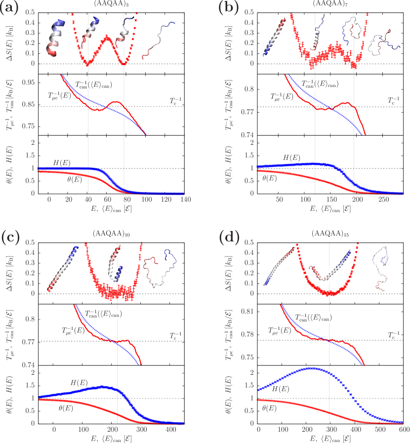
Figure 1:

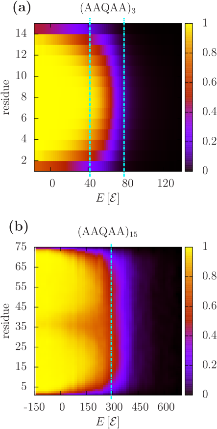
Figure 2:

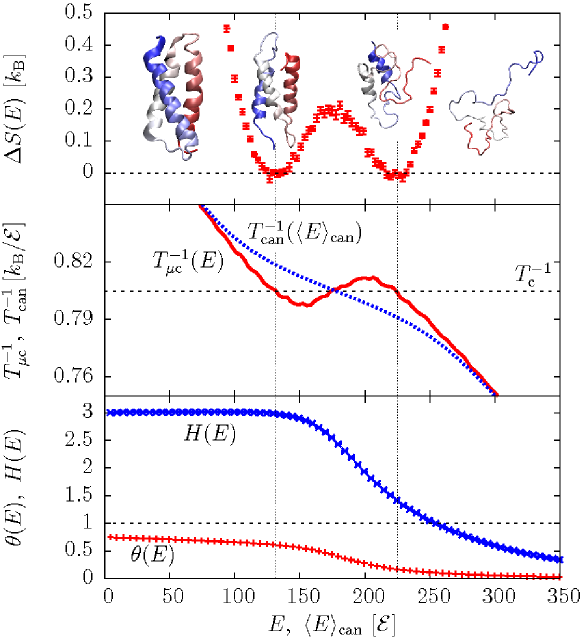
Figure 3:

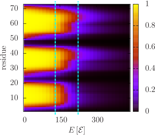
Figure 4:

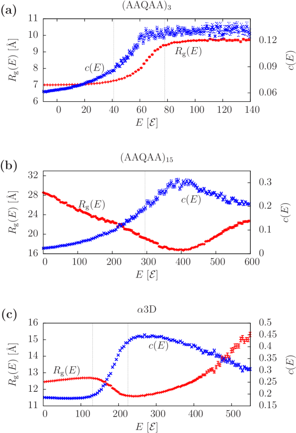
Figure 5:

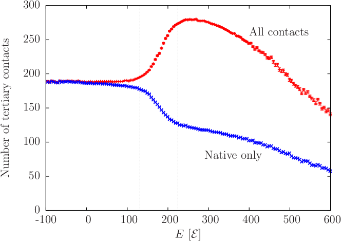
Figure 6:

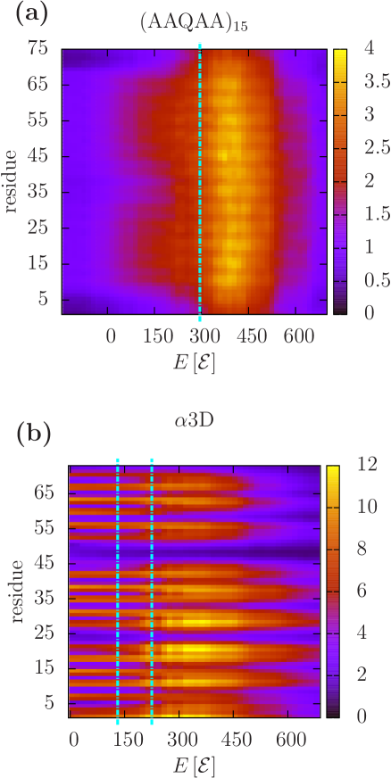
Figure 7:

References

- [1] Dobson, C. M., A. Šali, and M. Karplus. 1998. Protein folding: A perspective from theory and experiment. Angew. Chem. Int. Ed., 37:868–893.
- [2] Bryngelson, J. D., J. N. Onuchic, N. D. Socci, and P. G. Wolynes. 1995. Funnels, pathways, and the energy landscape of protein folding: A synthesis. Proteins: Struct. Funct. Bioinf., 21:167–195.
- [3] Jackson, S. E., 1998. How do small single-domain proteins fold? Fold. Des., 3:R81–R91.
- [4] Kaya, H., and H. S. Chan. 2000. Polymer principles of protein calorimetric two-state cooperativity. Proteins: Struct. Funct. Genet., 40:637–661.
- [5] Zhou, Y. Q., C. K. Hall, and M. Karplus. 1999. The calorimetric criterion for a two-state process revisited. Prot. Sci., 8:1064–1074.
- [6] Chan, H. S., S. Bromberg, and K. A. Dill. 1995. Models of cooperativity in protein folding. Philos. Trans. R. Soc. Lond. B Biol. Sci., 348:61–70.
- [7] Borgs, C., and S. Kappler. 1992. Equal weight versus equal height: A numerical study of an asymmetric first-order transition. Phys. Lett. A, 171:37–42.
- [8] Gross, D. H. E. 2001. Microcanonical Thermodynamics: Phase Transitions in ’Small’ Systems. World Scientific Publishing Company, 1st edition.
- [9] Hüller, A. 1994. First order phase transitions in the canonical and the microcanonical ensemble. Zeit. Phys. B, 93:401–405.
- [10] Deserno, M. 1997. Tricriticality and the Blume-Capel model: A Monte Carlo study within the microcanonical ensemble. Phys. Rev. E, 56:5204–5210.
- [11] Janke, W. 1998. Canonical versus microcanonical analysis of first-order phase transitions. Nucl. Phys. B - Proc. Supp., 63:631–633.
- [12] Hüller, A., and M. Pleimling. 2002. Microcanonical determination of the order parameter critical exponent. Int. J. Mod. Phys. C, 13:947–956.
- [13] Pleimling, M. and H. Behringer. 2005. Microcanonical analysis of small systems. Phase Transitions, 78:787–797.
- [14] Gross, D. H. E. 1993. Multifragmentation, link between fission and the liquid-gas phase-transition. Prog. Part. Nucl. Phys., 30:155–164.
- [15] Koonin, S. E., and J. Randrup. 1987. Microcanonical simulation of nuclear disassembly. Nucl. Phys. A, 474:173–192.
- [16] Fernández, L. A., V. Martín-Mayor, B. Seoane, and P. Verrocchio. 2010. Separation and fractionation of order and disorder in highly polydisperse systems. Phys. Rev. E, 82:021501–021507.
- [17] Komatsu, N., S. Kimura, and T. Kiwata. 2009. Negative specific heat in self-gravitating -body systems enclosed in a spherical container with reflecting walls. Phys. Rev. E, 80:041107–041115.
- [18] Posch. H. A., and W. Thirring. 2006. Thermodynamic instability of a confined gas. Phys. Rev. E, 74:051103–051108.
- [19] Chen, T., X. Lin, Y. Liu, and H. Liang. 2007. Microcanonical analysis of association of hydrophobic segments in a heteropolymer. Phys. Rev. E, 76:046110–046113.
- [20] Taylor, M. P., W. Paul, and K. Binder. 2009. All-or-none proteinlike folding transition of a flexible homopolymer chain. Phys. Rev. E, 79:050801–050804.
- [21] Hao, M. H., and H. A. Scheraga. 1994. Monte Carlo simulation of a first-order transition for protein folding. Journal Phys. Chem., 98:4940–4948.
- [22] Sikorski, A., and P. Romiszowski. 2003. Thermodynamical properties of simple models of protein-like heteropolymers. Biopolymers, 69:391–398.
- [23] Junghans, C., M. Bachmann, and W. Janke. 2006. Microcanonical analyses of peptide aggregation processes. Phys. Rev. Lett., 97:218103–218106.
- [24] Junghans, C., M. Bachmann, and W. Janke. 2008. Thermodynamics of peptide aggregation processes: An analysis from perspectives of three statistical ensembles. J. Chem. Phys., 128:085103–085111.
- [25] Hernandez-Rojas, J., and J. M. Gomez Llorente. 2008. Microcanonical versus canonical analysis of protein folding. Phys. Rev. Lett., 100:258104–258107.
- [26] Kim, J., T. Keyes, and J. E. Straub. 2009. Relationship between protein folding thermodynamics and the energy landscape. Phys. Rev. E, 79:030902(R).
- [27] Bereau, T., M. Bachmann, and M. Deserno. 2010. Interplay between secondary and tertiary structure formation in protein folding cooperativity. J. Am. Chem. Soc., 132:13129–13131.
- [28] Berg, B. A., and T. Neuhaus. 1991. Multicanonical algorithms for first order phase transitions. Phys. Lett. B, 267:249–253.
- [29] Wang, F., and D. P. Landau. 2001. Efficient, multiple-range random walk algorithm to calculate the density of states. Phys. Rev. Lett., 86:2050–2053.
- [30] Ferrenberg, A. M., and R. H. Swendsen. 1989. Optimized Monte Carlo data analysis. Phys. Rev. Lett., 63:1195–1198.
- [31] Kumar, S., D. Bouzida, R. H. Swendsen, P. A. Kollman, and J. M. Rosenberg. 1992. The weighted histogram analysis method for free-energy calculations on biomolecules. 1. The method. J. Comput. Chem., 13:1011–1021.
- [32] Bereau, T., and R. H. Swendsen. 2009. Optimized convergence for multiple histogram analysis. J. Comput. Phys., 228:6119–6129.
- [33] Swendsen, R. H., and J. S. Wang. 1986. Replica Monte-Carlo simulation of spin-glasses. Phys. Rev. Lett., 57:2607–2609.
- [34] Dill, K. A., and D. Stigter. 1995. Modeling protein stability as heteropolymer collapse. Adv. Prot. Chem., 46:59–104.
- [35] Baldwin, R. L. 1989. How does protein folding get started? Trends Biochem. Sci., 14, 291–294.
- [36] Bereau, T., and M. Deserno. 2009. Generic coarse-grained model for protein folding and aggregation. J. Chem. Phys., 130:235106–235120.
- [37] Limbach, H. J., A. Arnold, B. A. Mann, and C. Holm. 2006. ESPResSo - an extensible simulation package for research on soft matter systems. Comput. Phys. Comm., 174:704–727.
- [38] Walsh, S. T. R., H. Cheng, J. W. Bryson, H. Roder, and W. F. DeGrado. 1999. Solution structure and dynamics of a de novo designed three-helix bundle protein. Proc. Natl. Acad. Sci. USA, 96, 5486–5491.
- [39] Frishman, D., and P. Argos. 1995. Knowledge-based protein secondary structure assignment. Proteins: Struct. Funct. Genet., 23, 566–579.
- [40] Scholtz, J. M., E. J. York, J. M. Stewart, and R. L. Baldwin. 1991. A neutral, water-soluble, alpha-helical peptide: The effect of ionic-strength on the helix coil equilibrium. J. Am. Chem. Soc., 113, 5102–5104.
- [41] Shalongo, W., D. Laxmichand, and E. Stellwagen. 1994. Distribution of Helicity within the Model Peptide Acetyl(AAQAA)3amide. J. Am. Chem. Soc., 116, 8288–8293.
- [42] Zagrovic, B., G. Jayachandran, I. S. Millett, S. Doniach, and V. S. Pande. 2005. How Large is an -Helix? Studies of the Radii of Gyration of Helical Peptides by Small-angle X-ray Scattering and Molecular Dynamics. J. Mol. Biol., 353, 232–241.
- [43] Ferrara, P., J. Apostolakis, and A. Caflisch. 2000. Thermodynamics and kinetics of folding of two model peptides investigated by molecular dynamics simulations. J. Phys. Chem. B, 104:5000–5010.
- [44] Chebaro, Y., X. Dong, R. Laghaei, P. Derreumaux, and N. Mousseau. 2009. Replica exchange molecular dynamics simulations of coarse-grained proteins in implicit solvent. J. Phys. Chem. B, 113, 267–274.
- [45] Humphrey, W., A. Dalke, and K. Schulten. 1996. VMD: Visual molecular dynamics. J. Mol. Graphics, 14:33–38.
- [46] Privalov, P. L., 1989. Thermodynamic problems of protein structure. Annu. Rev. Biophys. Biophys. Chem., 18:47–69.
- [47] Privalov, P. L., 1982. Stability of proteins: Proteins which do not present a single cooperative system. Adv. Prot. Chem., 35:1–104.
- [48] Kaya, H., and H. S. Chan. 2000. Energetic components of cooperative protein folding. Phys. Rev. Lett., 85:4823–4826.
- [49] Ghosh, K., and K. A. Dill. 2009. Theory for protein folding cooperativity: Helix bundles. J. Am. Chem. Soc., 131:2306–2312.
- [50] Badasyan, A. V., G. N. Hayrapetyan, S. A. Tonoyan, Y. S. Mamasakhlisov, A. S. Benight, and V. F. Morozov. 2009. Intersegment interactions and helix-coil transition within the generalized model of polypeptide chains approach. J. Chem. Phys., 131:115104–115111.
- [51] Solc., K. 1971. Shape of a random-flight chain. J. Chem. Phys., 55, 335–344.
- [52] Sciutto, S. J. 1996. The shape of self-avoiding walks. J. Phys. A: Math. Gen., 29:5455–5473.
- [53] Hills Jr, R. D., and C. L. Brooks III. 2008. Subdomain competition, cooperativity, and topological frustration in the folding of chey. J. Mol. Biol., 382:485–495.
- [54] Privalov, P. L. 1979. Stability of proteins small globular proteins. Adv. Prot. Chem., 33:167–241.
- [55] Zimm, B. H., and J. K. Bragg. 1959. Theory of the phase transition between helix and random coil in polypeptide chains. J. Chem. Phys., 31:526–535.
- [56] Tiktopulo, E. I, V. E. Bychkova, J. Ricka, and O. B. Ptitsyn. 1994. Cooperativity of the coil-globule transition in a homopolymer: Microcalorimetric study of poly(n-isopropylacrylamide). Macromolecules, 27:2879–2882.
- [57] Zhu, Y., D. O. V. Alonso, K. Maki, C. Y. Huang, S. J. Lahr, V. Daggett, H. Roder, W. F. DeGrado, and F. Gai. 2003. Ultrafast folding of alpha(3): A de novo designed three-helix bundle protein. Proc. Natl. Acad. Sci. USA, 100:15486–15491.
- [58] Nettels, D., S. Müller-Späth, F. Küster, H. Hofmann, D. Haenni, S. Rüegger, L. Reymond, A. Hoffmann, J. Kubelka, B. Heinz, K. Gast, R. B. Best, and B. Schuler. 2009. Single-molecule spectroscopy of the temperature-induced collapse of unfolded proteins. Proc. Natl. Acad. Sci. USA, 106:20740–20745.
- [59] Chan, H. S. 2000. Modeling protein density of states: Additive hydrophobic effects are insufficient for calorimetric two-state cooperativity. Proteins: Struct. Funct. Genet., 40:543–571.
- [60] Booth, D. R., 1997. Instability, unfolding and aggregation of human lysozyme variants underlying amyloid fibrillogenesis Nature, 385:787–793.