Solitary waves and their linear stability in nonlinear lattices

Solitary waves in a general nonlinear lattice are discussed, employing as a model the nonlinear Schrödinger equation with a spatially periodic nonlinear coefficient. An asymptotic theory is developed for long solitary waves, that span a large number of lattice periods. In this limit, the allowed positions of solitary waves relative to the lattice, as well as their linear stability properties, hinge upon a certain recurrence relation which contains information beyond all orders of the usual two-scale perturbation expansion. It follows that only two such positions are permissible, and of those two solitary waves, one is linearly stable and the other unstable. For a cosine lattice, in particular, the two possible solitary waves are centered at a maximum or minimum of the lattice, with the former being stable, and the analytical predictions for the associated linear stability eigenvalues are in excellent agreement with numerical results. Furthermore, a countable set of multi-solitary-wave bound states are constructed analytically. In spite of rather different physical settings, the exponential asymptotics approach followed here is strikingly similar to that taken in earlier studies of solitary wavepackets involving a periodic carrier and a slowly-varying envelope, which underscores the general value of this procedure for treating multi-scale solitary-wave problems.

1 Introduction

The nonlinear Schrödinger (NLS) equation is fundamental to wave propagation in fluid flows, optics, Bose–Einstein condensation (BEC) and applied mathematics [2, 3, 4, 5, 6, 7]. When a linear periodic potential (so-called linear lattice) is added, the resulting equation then models nonlinear beam transmission in an optical medium with a periodic transverse variation in the linear refractive index, and atom–atom interaction in Bose–Einstein condensates loaded in an optical lattice [8, 9, 10, 11]. Another interesting possibility, instead of a linear lattice, is to allow the nonlinear coefficient of the NLS equation to vary periodically in space. In optics, such a periodic nonlinear coefficient (also called nonlinear lattice) would arise in the propagation of laser beams in a medium whose nonlinear refractive index is modulated in the transverse direction. The same model equation also applies to the study of Bose–Einstein condensates in a medium with a spatially-dependent scattering length. In optical and BEC experiments, a linear lattice can be created by beam interference [9, 12]. A nonlinear lattice in optics can be created by femtosecond-laser writing in fused silica [13], and in BEC such a lattice can be created by an optical Feshbach-resonance modulation of the scattering length [14, 15, 16]. Wave phenomena in linear lattices have been extensively studied in the past decade (see [11] for a review). In this paper, our interest centers on wave phenomena in nonlinear lattices.

Wave phenomena in symmetric nonlinear lattices have been investigated in [17, 18, 19]. It was found that there exist solitary waves which are centered at a local maximum or minimum of the nonlinear lattice. Short solitary waves were found to be stable/unstable when centered at a local maximum/minimum of the lattice [18, 19], but the stability analysis for long solitary waves, that extend over a large number of lattice periods, was not conclusive [18]. Bound states comprising several fundamental solitary waves have also been reported numerically [17]. In addition to these studies in nonlinear lattices, work has also been done in the presence of both linear and nonlinear lattices [20, 21, 22] and in higher dimensions [23].

In this paper, we make an analytical study of long solitary waves and their linear stability properties in a general nonlinear lattice. Recognizing that the coupling between a long solitary wave and the relatively short nonlinear lattice is an exponentially small effect, beyond all orders of the usual multiple-scale perturbation expansion in powers of the long-wave parameter, our analysis makes use of an exponential asymptotics technique. We show that long solitary waves can only be located at two positions in one period of the nonlinear lattice, regardless of the number of local maxima and minima in it. If the lattice is symmetric, the solitary-wave positions are simply the point of symmetry and half a lattice-period away from it; but for a general asymmetric lattice, these positions need to be determined by solving a certain recurrence relation that contains information beyond all orders of the long-wave parameter. Linear stability analysis of long solitary waves is also performed: it follows from the same recurrence relation that one of the two solitary waves is linearly stable, while the other is unstable. For cosine lattices, in particular, the solitary wave centered at the maximum/minimum of the lattice is linearly stable/unstable, consistent with previous results [18, 19]. An analytical formula for the linear-stability eigenvalues is also derived; as expected, these eigenvalues are exponentially small in the long-wave parameter. The analytical predictions for the stability eigenvalues are compared with direct numerical results and excellent agreement is obtained. Lastly, we also show that an infinite number of multi-solitary-wave stationary bound states exist in the nonlinear lattice, and their analytical construction in terms of nonlocal solitary waves is presented.

The exponential asymptotics procedure adopted in this paper closely resembles that used in recent studies [24, 25] of gap solitons in a linear lattice (see also [26, 27] for the first application of this technique to solitary wavepackets of the fifth-order KdV equation). The common thread in linear and nonlinear lattices is that the solitary wave is much longer than the period of the underlying lattice; hence, the coupling between these different scales is expected to be exponentially small, which invites similar exponential asymptotics treatment. As a result, the behavior of solitary waves in these rather different physical settings is remarkably similar.

2 Preliminaries

We study the NLS equation with a nonlinear lattice

$$i\Psi_{t}+\Psi_{zz}+(1+g(z/\epsilon))|\Psi|^{2}\Psi=0\,,$$ (2.1)

where $g(z/\epsilon)$ is a periodic function which describes the spatial variation of the nonlinear Kerr coefficient, and the parameter $\epsilon>0$ controls the length scale of this variation. Throughout this article, $g(z/\epsilon)$ will be referred to as the nonlinear lattice. Eq. (2.1) is a model for the spatial propagation of a laser beam in a medium whose nonlinear refractive index is modulated periodically in the transverse direction (in this context, $t$ is the direction of propagation), and for the dynamics of Bose–Einstein condensates whose scattering length (the counterpart of the nonlinear coefficient in (2.1)) changes periodically over space [5, 16]. Solitary-wave solutions in Eq. (2.1) and their linear-stability properties for even functions of $g(z/\epsilon)$ were investigated in [18, 19]. In the long-wave limit $(\epsilon\ll 1)$, profiles of solitary waves that span many lattice periods were determined by a multiscale perturbation analysis [18], but their stability was not ascertained.

In this article, we analytically study long solitary waves ($0<\epsilon\ll 1$) and their stability properties for general forms of the nonlinear lattice $g(z/\epsilon)$. Specifically, denoting $z/\epsilon=x$, $g(x)$ is assumed to be periodic with period $d$,

$$g(x+d)=g(x)$$ (2.2)

for all real values of $x$. Also, without loss of generality, $g(x)$ is taken to have zero $x$-average:

$$\langle g\rangle\equiv\frac{1}{d}\int_{0}^{d}g(x){\rm d}x=0\,.$$ (2.3)

Solitary-wave solutions of Eq. (2.1) are sought in the form

$$\Psi(z,t)=\psi(z){\rm e}^{i\mu t}\,,$$ (2.4)

where $\mu>0$ is the propagation constant, and the real-valued function $\psi(z)$ solves the ordinary differential equation

$$\psi_{zz}+(1+g(z/\epsilon))\psi^{3}-\mu\psi=0\,,$$ (2.5)

under the boundary condition of $\psi\to 0$ as $|z|\to\infty$.

Here, we will fix $\mu=O(1)$, and determine the solitary wave $\psi(z)$ as well as its linear stability for $0<\epsilon\ll 1$. In this regime, the nonlinear lattice $g(z/\epsilon)$ is rapidly varying and the wave profile $\psi(z)$, whose width is $O(1)$ for $\mu=O(1)$, spans many lattice sites. As $\epsilon\to 0$, $g(z/\epsilon)$ features extremely rapid oscillations with zero mean and the effect of the nonlinear lattice on the solitary wave $\psi(z)$ can be dropped; thus, in this limit, $\psi(z)$ is expected to approach the familiar solitary-wave solution of the lattice-free NLS equation

$$\psi(z)\to a\mathop{\rm sech}\nolimits{z-z_{0}\over\beta}\,,$$ (2.6)

where

$$a=\sqrt{2\mu},\quad\beta=1/\sqrt{\mu},$$ (2.7)

and $z_{0}$ denotes the location of the peak of the solitary wave $\psi(z)$. When $0\neq\epsilon\ll 1$, the nonlinear lattice $g(z/\epsilon)$ will have a weak but non-negligible effect, and solitary waves bifurcate out from the limiting wave (2.6); this bifurcation will be the main focus of our investigation. It will be shown that such a bifurcation is possible only when $z_{0}$ takes two special values relative to the nonlinear lattice, resulting in two solitary-waves, out of which one is stable and the other unstable.

It is worth mentioning that a different but equivalent analysis is to introduce scaled variables

$$\widehat{\psi}=\epsilon\psi,\quad x=z/\epsilon,\quad\widehat{\mu}=\epsilon^{2}\mu,$$ (2.8)

so that Eq. (2.5) transforms into

$$\widehat{\psi}_{xx}+(1+g(x))\hskip 1.13791pt\widehat{\psi}^{3}-\widehat{\mu}\widehat{\psi}=0\,.$$ (2.9)

Thus, fixing $\mu=O(1)$ and varying $\epsilon\ll 1$ in our treatment above corresponds to fixing the lattice $g(x)$ and varying $\widehat{\mu}\ll 1$ in Eq. (2.9). In this alternative treatment, the nonlinear lattice $g(x)$ is no longer rapidly varying, but for $\widehat{\mu}\ll 1$, solitary waves $\widehat{\psi}(x)$ of Eq. (2.9) that bifurcate out from the edge $\widehat{\mu}_{0}=0$ of the continuous spectrum (whose linear eigenmode is a constant) have low amplitude and are long compared to the lattice period. This type of solitary-wave bifurcation is akin to that studied in [24] with a linear lattice. In both treatments, however, the solitary wave is of long extent and spans many lattice sites, hence the fundamental feature of the problem remains the same.

3 Multiscale perturbation solution

We begin by reviewing the multiple-scale procedure followed in [18] for solving equation (2.5). The solution $\psi$ to this equation contains two scales, reflected in the ‘slow’ variable $z$ and ‘fast’ variable $x=z/\epsilon$. Introducing explicitly these variables by writing $\psi=\psi(x,z)$, Eq. (2.5) then becomes

$$\bigg{(}\partial^{2}_{z}+\frac{2}{\epsilon}\partial_{x}\partial_{z}+\frac{1}{\epsilon^{2}}\partial^{2}_{x}\bigg{)}\,\psi+(1+g(x))\psi^{3}-\mu\psi=0\,.$$ (3.1)

Now we expand $\psi(x,z)$ into the two-scale perturbation series,

$$\psi(x,z)=\psi_{0}(x,z)+\epsilon\psi_{1}(x,z)+\epsilon^{2}\psi_{2}(x,z)+\cdots\,.$$ (3.2)

Substituting this expansion into Eq. (3.1) and from various orders of $\epsilon$, we get the following hierarchy of equations,

$$-\partial^{2}_{x}\psi_{0} =0\,,$$ (3.3a)

$$-\partial^{2}_{x}\psi_{1} =2\partial_{x}\partial_{z}\psi_{0}\,,$$ (3.3b)

$$-\partial^{2}_{x}\psi_{2} =\partial^{2}_{z}\psi_{0}+2\partial_{x}\partial_{z}\psi_{1}+(1+g(x))\psi^{3}_{0}-\mu\psi_{0}\,,$$ (3.3c)

$$-\partial^{2}_{x}\psi_{3} =\partial^{2}_{z}\psi_{1}+2\partial_{x}\partial_{z}\psi_{2}+3(1+g(x))\psi^{2}_{0}\psi_{1}-\mu\psi_{1}\,,$$ (3.3d)

$$-\partial^{2}_{x}\psi_{4} =\partial^{2}_{z}\psi_{2}+2\partial_{x}\partial_{z}\psi_{3}+3(1+g(x))\psi^{2}_{0}\psi_{2}+3(1+g(x))\psi_{0}\psi^{2}_{1}-\mu\psi_{2}\,.$$ (3.3e)

From Eq. (3.3a) and the requirement that $\psi_{0}$ be bounded, we get

$$\psi_{0}=\tilde{\psi}_{0}(z).$$ (3.4)

Substituting this equation into (3.3b) and requiring $\psi_{1}$ to be bounded, we get

$$\psi_{1}=\tilde{\psi}_{1}(z).$$ (3.5)

Equations (3.3c)–(3.3e) are forced linear equations and can be written in the unified form

$$-\partial^{2}_{x}\psi_{n}=Q_{n}(x,z)\,,$$ (3.6)

where $Q_{n}$ depends on $\psi_{j}$ with $j<n$. The $x$-dependence of $Q_{n}$ derives from the nonlinear lattice $g(x)$ which is $d$-periodic. Thus $Q_{n}$ is $d$-periodic in $x$ and can be expanded into a Fourier series,

$$Q_{n}(x,z)=\sum_{m=-\infty}^{\infty}q_{m}(z){\rm e}^{2\pi imx/d}.$$ (3.7)

We require solutions $\psi_{n}$ to be also $d$-periodic in $x$. The necessary and sufficient condition for the existence of such a solution is that the constant Fourier mode $q_{0}$ in (3.7) vanish,

$$q_{0}=\langle Q_{n}\rangle=0\,.$$ (3.8)

Here $\langle\cdot\rangle$ is the average with respect to $x$ as defined in (2.3). Then the solution $\psi_{n}$ to Eq. (3.6) is

$$\psi_{n}=-\partial^{-2}_{x}Q_{n}(x,z)+\tilde{\psi}_{n}(z)\,,$$ (3.9)

where

$$\partial^{-2}_{x}Q_{n}=\sum_{m\neq 0}\bigg{(}{2\pi im\over d}\bigg{)}^{-2}q_{m}(z){\rm e}^{2\pi imx/d}\,,$$ (3.10)

and $\tilde{\psi}_{n}$ is a function of $z$ which is determined by the solvability condition (3.8) for the equation governing $\psi_{n+2}$ (see below).

Next we determine $\tilde{\psi}_{0}(z)$ and $\tilde{\psi}_{1}(z)$. Specifically, to obtain $\tilde{\psi}_{0}(z)$, we return to equation (3.3c). Substituting (3.5) into (3.3c) and recalling that $g(x)$ has zero average (see (2.3)), the solvability condition of this equation gives

$$\partial^{2}_{z}\tilde{\psi}_{0}+\tilde{\psi}_{0}^{3}-\mu\tilde{\psi}_{0}=0\,,$$ (3.11)

whose solution is

$$\tilde{\psi}_{0}=A(z)\equiv a\mathop{\rm sech}\nolimits{z-z_{0}\over\beta},$$ (3.12)

where $a$ and $\beta$ are defined in (2.7), and $z_{0}$ is a constant. This result agrees with (2.6), as anticipated earlier.

To determine the solution $\tilde{\psi}_{1}(z)$, we consider equation (3.3d). Using the above expression for $\tilde{\psi}_{0}$ and the zero average of $g(x)$, the solvability condition for (3.3d) gives

$$\left({{\rm d}^{2}/{\rm d}z^{2}}-\mu+3A^{2}\right)\tilde{\psi}_{1}=0\,,$$ (3.13)

whose solution is

$$\tilde{\psi}_{1}=\zeta A^{\prime}(z),$$ (3.14)

where $\zeta$ is a constant. It is clear that $\tilde{\psi}_{1}$ simply shifts the location of the center of the leading-order term, $\tilde{\psi}_{0}=A(z)$, in the perturbation expansion (3.2). To remove the ambiguity in the position of $\tilde{\psi}_{0}$, we require that $\tilde{\psi}_{1}$ be orthogonal to $\tilde{\psi}_{0}$, hence $\zeta=0$, and

$$\tilde{\psi}_{1}(z)=0.$$ (3.15)

Now we determine the solution $\psi_{2}$ to Eq. (3.3c). Utilizing solutions $\psi_{0}$ and $\psi_{1}$ in Eqs. (3.12) and (3.15), $\psi_{2}$ can be written as

$$\psi_{2}(x,z)=-[\partial^{-2}_{x}g(x)]A^{3}(z)+\tilde{\psi}_{2}(z)\,.$$ (3.16)

When this solution is inserted into equation (3.3e), the solvability condition of this equation gives

$$\left({{\rm d}^{2}/{\rm d}z^{2}}-\mu+3A^{2}\right)\tilde{\psi}_{2}=-3\alpha A^{5}\,,$$ (3.17)

where

$$\alpha\equiv\langle(\partial^{-1}_{x}g)^{2}\rangle>0.$$ (3.18)

The bounded solution $\tilde{\psi}_{2}$ to this equation is

$$\tilde{\psi}_{2}(z)=\alpha(A^{3}-2a^{2}A).$$ (3.19)

Combining  (3.4),  (3.5),  (3.15),  (3.16) and  (3.19), the perturbation series solution for the solitary wave $\psi(x,z)$ of Eq. (2.5) takes the form

$$\psi(x,z)=A(z)+\epsilon^{2}\bigg{\{}-\left[\partial^{-2}_{x}g(x)\right]A^{3}(z)+\alpha\left[A^{3}(z)-2a^{2}A(z)\right]\bigg{\}}+O(\epsilon^{3})\,,$$ (3.20)

where $A(z)$ is given by (3.12).

Notice that the location $z_{0}$ of the peak of the function $A(z)$ in Eq. (3.20) is arbitrary at this stage, since equation (3.11) which determines $A(z)$ is translation invariant. However, the original equation (2.5) for the solitary wave is not translation invariant due to the presence of the nonlinear lattice $g(x)$, and it is unlikely that the solitary wave can be arbitrarily located relative to this nonlinear lattice. Indeed, a very similar situation arises in a linear lattice [7, 24, 28], and there it was shown that solitary waves can only be located at two positions relative to the lattice. In the present problem, the result turns out to be similar: only two values of $z_{0}$ are permissible for truly localized solitary waves in a nonlinear lattice, as will be established in the next section by utilizing exponential asymptotics.

Before ending this section, it should be pointed out that truly localized solitary waves $\psi(z)$ of Eq. (2.5) must satisfy

$$\int_{-\infty}^{\infty}g^{\prime}(z/\epsilon)\psi^{4}(z)dz=0.$$ (3.21)

This constraint can be obtained by multiplying Eq. (2.5) with $\psi^{\prime}(z)$ and then integrating from $-\infty$ to $\infty$. An analogous constraint was noted in [28] for the linear lattice problem, and it was pointed out that, if the lattice is symmetric, this constraint predicts only two possible locations for truly localized solitary waves — one at the point of symmetry and the other half a period away from it [7, 28]. But for general asymmetric linear lattices, it does not seem feasible to determine the locations of solitary waves based on this constraint alone [24]. Similarly, in the problem at hand, if the nonlinear lattice $g(z/\epsilon)$ is symmetric, the constraint (3.21) can also predict the two locations of true solitary waves; if the lattice is asymmetric, however, this approach would again fail. The reason is that, when the perturbation series solution (3.20) is substituted into the constraint (3.21), all terms in the series make contributions of the same order of magnitude to the integral in (3.21). Hence it does not seem possible to solve for $z_{0}$ without having obtained all terms in the perturbation series (3.20). The same difficulty also appears in the linear lattice problem [7, 24] and suggests the need for a perturbation theory beyond all orders. This task is taken up below by employing an exponential-asymptotics procedure in the wavenumber domain [24, 26].

4 Growing tails of exponentially small amplitude

In this section, we determine the location of the solitary wave $\psi(z)$ by the exponential asymptotics method. Our approach closely resembles that for gap solitons in a linear lattice [24], thus only the key ideas and steps will be given. For further details, we refer the reader to [24] (see also [26]).

The ensuing analysis is based on the fact that, if $\psi(z)$ given by (3.20) is required to decay upstream ($z\ll-1$), then this solution of Eq. (2.5) will contain a growing tail downstream ($z\gg 1$) for generic values of the position $z_{0}$ of the solitary wave core. Specifically, if the upstream asymptotics of $\psi(z)$, as given by the leading-order term in the perturbation expansion (3.20), is

$$\psi\sim 2a\,{\rm e}^{(z-z_{0})/\beta},\qquad z\to-\infty\,,$$ (4.1)

then the downstream asymptotics of the solution will be

$$\psi\sim 2a\,{\rm e}^{-(z-z_{0})/\beta}+H\,{\rm e}^{(z-z_{0})/\beta},\qquad z\gg 1\,,$$ (4.2)

where $H(\epsilon,z_{0})$ is the growing-tail amplitude. As we will show later, $H$ vanishes only at two special values of $z_{0}$ (relative to the nonlinear lattice), thus only two truly-localized solitary waves exist. The tail amplitude $H(\epsilon,z_{0})$ turns out to be exponentially small in $\epsilon$, so this growing tail can not be captured by the perturbation series (3.20) and has to be obtained by carrying this expansion in powers of $\epsilon$ beyond all orders.

Following the exponential asymptotics procedure in the wavenumber domain [24], we introduce the Fourier transform of $\psi(x,z)$ with respect to the slow variable $z$,

$$\widehat{\psi}(x,K)={1\over 2\pi}\int_{-\infty}^{\infty}\psi(x,z){\rm e}^{-iKz}{\rm d}z\,.$$ (4.3)

Substituting the perturbation series solution (3.20) for $\psi(x,z)$ into this Fourier transform, we find that

$$\widehat{\psi}(x,K)={\sqrt{2}\over 2}{\rm e}^{-iKz_{0}}\mathop{\rm sech}\nolimits\bigg{(}{\pi\over 2}\beta K\bigg{)}\left\{1+\epsilon^{2}a^{2}\,\left[{1\over 2}(1+\beta^{2}K^{2})\nu(x)-2\alpha\right]+\cdots\right\}\,,$$ (4.4)

where $\nu(x)=\alpha-\partial^{-2}_{x}g(x)$. This expansion in the wavenumber domain is disordered when $K=O(1/\epsilon)$, suggesting that $\widehat{\psi}$ has pole singularities at $K=O(1/\epsilon)$. The residues of these singularities are exponentially small due to the exponentially small value of the sech function in (4.4) at $K=O(1/\epsilon)$. As we will show later, these singularities of exponentially-small residue contribute exponentially-small but growing tails in the physical solution $\psi(x,z)$. Thus the main goal is to determine the locations and residues of pole singularities in $\widehat{\psi}$.

To this end, we replace the disordered expansion (4.4) by a uniformly-valid expression,

$$\widehat{\psi}={\rm e}^{-iKz_{0}}\mathop{\rm sech}\nolimits\bigg{(}{\pi\over 2}\beta K\bigg{)}U(x,\kappa)\,,$$ (4.5)

where $\epsilon K=\kappa$. We then take the Fourier transform of Eq. (3.1) with respect to $z$,

$$\widehat{\psi}_{xx}+2i\kappa\widehat{\psi}_{x}-\kappa^{2}\widehat{\psi}+\epsilon^{2}(1+g(x))\widehat{\psi^{3}}-\epsilon^{2}\mu\,\widehat{\psi}=0\ ,$$ (4.6)

and upon substituting Eq. (4.5) into (4.6), we obtain the following equation for $U$

$$U_{xx} +2i\kappa U_{x}-\kappa^{2}U-\epsilon^{2}\mu U$$

$$+(1+g(x))\cosh{\pi\beta\over 2}K\int_{-\infty}^{\infty}{\rm d}\lambda{U(x,\kappa-\lambda)\over\cosh{\pi(\kappa-\lambda)\beta\over 2\epsilon}}\int_{-\infty}^{\infty}{\rm d}\rho{U(x,\lambda-\rho)U(x,\rho)\over\cosh{\pi(\lambda-\rho)\beta\over 2\epsilon}\cosh{\pi\rho\beta\over 2\epsilon}}=0\,.$$ (4.7)

4.1 The recurrence equation

In the limit $\epsilon\to 0$ and for $\kappa$ away from singularities of $U(x,\kappa)$, the main contribution to the double integral in Eq. (4.7) comes from $0<\lambda<\kappa$ when $\kappa>0$ and from $\kappa<\lambda<0$ when $\kappa<0$. The integral equation (4.7) then simplifies to [24, 26]

$$U_{xx}+2i\kappa U_{x}-\kappa^{2}U+4(1+g(x))\int_{0}^{\kappa\!\!}{\rm d}\lambda U(x,\kappa-\lambda)\int_{0}^{\lambda\!\!}{\rm d}\rho U(x,\lambda-\rho)U(x,\rho)=0\,.$$ (4.8)

The solution to this simplified integral equation can be posed as a power series in $\kappa$,

$$U(x,\kappa)={\sqrt{2}\over 2}\sum_{n=0}^{\infty}U_{n}(x)\kappa^{n}\,.$$ (4.9)

Substituting this power series into (4.8), we obtain the following recurrence equation for $U_{n}$,

$${{\rm d}^{2}U_{n+2}\over{\rm d}x^{2}}= \ U_{n}-2i{{\rm d}U_{n+1}\over{\rm d}x}$$

$$-2(1+g(x))\sum_{m=0}^{n}U_{n-m}{(n-m)!\over(n+2)!}\sum_{r=0}^{m}U_{r}U_{m-r}r!(m-r)!\,.$$ (4.10)

To be consistent with (4.4), we set

$$U_{0}=1,\quad U_{1}=0,$$ (4.11)

which serve as the initial conditions for the recurrence iteration (4.10). Note that this recurrence system does not involve $\mu$ and $\epsilon$; it only depends on the functional form of the periodic lattice $g(x)$.

4.2 Behavior near singularities

When $\kappa$ is near the singularities of $U(x,\kappa)$, the reduced integral equation (4.8) does not apply. We now examine the behavior of $U(x,\kappa)$ near its singularities, based on the original integral equation (4.7).

These singularities occur at $\kappa\approx\kappa_{0}$, where the linear part of Eq. (4.7) is satisfied, i.e.,

$$U_{xx}+2i\kappa_{0}U_{x}-\kappa^{2}_{0}U=0\,.$$ (4.12)

The bounded solution to this linear equation is $U\sim{\rm e}^{-i\kappa_{0}x}$. Since $U$ is expected to be $d$-periodic in $x$ in view of (4.5), therefore, $\kappa_{0}=\pm 2\pi/d$. Singularities near $\kappa_{0}=\pm 4\pi/d,\pm 6\pi/d,\dots$ are also possible, but they are subdominant and will not be considered. To avoid ambiguity, we denote

$$\kappa_{0}=2\pi/d\,,$$ (4.13)

and examine singularities at $\kappa\approx\pm\kappa_{0}$.

In order to determine the behavior of the solution $U$ near the singularity $\kappa\approx\kappa_{0}$, we first introduce the ‘inner’ wavenumber

$$\xi={\kappa-\kappa_{0}\over\epsilon}\,,$$ (4.14)

that is, $\kappa=\kappa_{0}+\epsilon\xi$ with $\xi=O(1)$. Guided by the analysis in [24, 26], we expand

$$U={{\rm e}^{-i\kappa_{0}x}\over\epsilon^{4}}\big{(}\Phi_{0}(\xi)+\epsilon^{2}f(x,\xi)+\cdots\big{)}\,.$$ (4.15)

The reason for the leading-order term in this expansion being $O(\epsilon^{-4})$ will be explained later (see Eq. (4.22)).

Now we examine the integral equation (4.7) near the singularity $\kappa\approx\kappa_{0}$. The dominant contributions to the double integral in (4.7) come from the following regions: (i) $\lambda\sim 0$ and $\rho\sim 0$, (ii) $\lambda\sim\kappa$ with $\rho\sim 0$ and with $\rho\sim\kappa$. Taking into account the leading-order term near $\kappa\sim\kappa_{0}$ in (4.15) and the leading order term near $\kappa\sim 0$ in (4.9), we can calculate these dominant contributions, and Eq. (4.7) near $\kappa\sim\kappa_{0}$ yields

$$\tilde{U}_{xx}+2i\epsilon\xi\tilde{U}_{x}-\epsilon^{2}\xi^{2}\tilde{U}-\epsilon^{2}\mu\tilde{U}+{3(1+g(x))\over\epsilon^{2}}\int_{-\infty}^{\infty}\omega{\rm e}^{\pi\beta\omega/2}\mathop{\rm csch}\nolimits{\pi\beta\omega\over 2}\Phi_{0}(\xi-\omega)\hskip 1.13791pt{\rm d}\omega=0\,,$$ (4.16)

where $U={\rm e}^{-i\kappa_{0}x}\tilde{U}$. Substituting the expansion  (4.15) into  (4.16), the terms of $O(\epsilon^{-4})$ and $O(\epsilon^{-3})$ are automatically balanced. At $O(\epsilon^{-2})$ we have

$$\partial^{2}_{x}f=\xi^{2}\Phi_{0}(\xi)+\mu\Phi_{0}(\xi)-3(1+g(x))\int_{-\infty}^{\infty}\omega{\rm e}^{\pi\beta\omega/2}\mathop{\rm csch}\nolimits{\pi\beta\omega\over 2}\Phi_{0}(\xi-\omega)\hskip 1.13791pt{\rm d}\omega\ ,$$ (4.17)

and the solvability condition requires that the $x$-average of the right-hand side of Eq. (4.17) equals to zero:

$$(\mu+\xi^{2})\Phi_{0}(\xi)-3\int_{-\infty}^{\infty}\omega{\rm e}^{\pi\beta\omega/2}\mathop{\rm csch}\nolimits{\pi\omega\beta\over 2}\Phi_{0}(\xi-\omega)\hskip 1.42271pt{\rm d}\omega=0\,.$$ (4.18)

Recalling that $\beta=1/\sqrt{\mu}$, this integral equation is identical to that encountered earlier in our analysis of gap solitons in a linear lattice  [24]. Hence, its solution is [24, 26]

$$\Phi_{0}(\xi)={6\beta^{4}\over 1+\beta^{2}\xi^{2}}\int_{\cal L^{\pm}}{1\over\sin^{2}s}\phi(s)e^{-s\beta\xi}{\rm d}s,$$ (4.19)

where

$$\phi(s)=C\bigg{(}{2\over\sin s}+{\cos^{2}s\over\sin s}-{3s\cos s\over\sin^{2}s}\bigg{)},$$ (4.20)

the contours $\cal L^{\pm}$ extend from $0$ to $\pm i\infty$ for $\mbox{Im}(\xi)<0$ and $\mbox{Im}(\xi)>0$ respectively, and $C$ is a complex constant which will be determined later. Note that the function $\Phi_{0}(\xi)$ given by (4.19) is analytic everywhere in the complex plane ${\mathbb{C}}$, save for two simple poles at $\xi=\pm i/\beta$. Also, $\Phi_{0}(\xi)$ satisfies the integral equation (4.18) only in the complex $\xi$-plane outside the strip $-1/\beta<\mbox{Im}(\xi)<1/\beta$, as was explained in [24].

The behavior of the function $\Phi_{0}(\xi)$ near its singularities $\xi=\pm i/\beta$ is

$$\Phi_{0}(\xi)\to-\frac{C\beta^{4}}{1+\beta^{2}\xi^{2}}\qquad(\xi\to\mp\frac{i}{\beta}),$$ (4.21)

and its large-$\xi$ asymptotics is  [24, 26]

$$\Phi_{0}(\xi)\to{12C\over 5}{1\over\xi^{4}}\qquad(\xi\to\infty)\,.$$ (4.22)

This fourth-order algebraic decay rate of $\Phi_{0}(\xi)$ at large $\xi$ implies the order $\epsilon^{-4}$ in Eq. (4.15). From Eq. (4.21), we then obtain the behavior of $\widehat{\psi}(x,K)$ near $K=\kappa_{0}/\epsilon\mp i/\beta$ as

$$\widehat{\psi}\sim{\beta^{3}C\over\epsilon^{3}}e^{-\pi\beta\kappa_{0}/2\epsilon}e^{\mp z_{0}/\beta}{e^{-i\kappa_{0}(x+x_{0})}\over K-{\kappa_{0}\over\epsilon}\pm{i\over\beta}}\qquad(K\to{\kappa_{0}\over\epsilon}\mp{i\over\beta})\,.$$ (4.23)

From the symmetry of the Fourier transform for real functions, $\widehat{\psi}$ is also singular at $K=-\kappa_{0}/\epsilon\mp i/\beta$, and

$$\widehat{\psi}\sim-{\beta^{3}C^{*}\over\epsilon^{3}}e^{-\pi\beta\kappa_{0}/2\epsilon}e^{\mp z_{0}/\beta}{e^{i\kappa_{0}(x+x_{0})}\over K+{\kappa_{0}\over\epsilon}\pm{i\over\beta}}\qquad(K\to-{\kappa_{0}\over\epsilon}\mp{i\over\beta})\,.$$ (4.24)

4.3 The growing tail and locations of solitary waves

We now take the inverse Fourier transform of $\widehat{\psi}(x,K)$ in order to calculate the growing tails in $\psi(x,z)$ due to the pole singularities (4.23)– (4.24). The inverse Fourier transform is

$$\psi(x,z)=\int_{\cal C}\widehat{\psi}(x,K)e^{iKz}{\rm d}K\,,$$ (4.25)

where the contour $\cal C$ is taken along the line $\Im(K)=-1/\beta$ and to pass below the poles at $K=\pm\kappa_{0}/\epsilon-i/\beta$ (the reason for this choice of the contour is explained in [24]). Also, the contour $\cal C$ passes above the pole of $\mathop{\rm sech}\nolimits(\pi\beta K/2)$ at $K=-i/\beta$, to be consistent with the desired upstream behavior of $\psi$ in (4.1).

Indeed, for $z\ll-1$, the dominant contribution to the inverse Fourier transform (4.25) comes from the pole of $\mathop{\rm sech}\nolimits(\pi\beta K/2)$ at $K=-i/\beta$ and one obtains the upstream solution (4.1). On the other hand, for $z\gg 1$, both the singularities (4.23)– (4.24) at $K=\pm\kappa_{0}/\epsilon-i/\beta$ and the singularity of $\mathop{\rm sech}\nolimits(\pi\beta K/2)$ at $K=i/\beta$ contribute, and one obtains the downstream solution behavior as

$$\psi\sim 2a{\rm e}^{-(z-z_{0})/\beta}+{4\pi\beta^{3}\widehat{C}\over\epsilon^{4}}{\rm e}^{-\pi\beta\kappa_{0}/2\epsilon}\sin(\kappa_{0}x_{0}-\theta){\rm e}^{(z-z_{0})/\beta}\qquad(z\gg 1)\,,$$ (4.26)

where $\widehat{C}>0$ and $\theta$ are the amplitude and phase of the complex constant $C$,

$$C=\widehat{C}{\rm e}^{i\theta}\,.$$ (4.27)

Equation (4.26) is one of the key results in this paper. It shows that a growing tail of exponentially small amplitude appears far downstream in the solution $\psi(x,z)$, except when

$$\sin(\kappa_{0}x_{0}-\theta)=0\,,$$ (4.28)

i.e.,

$$x_{0}=\theta/\kappa_{0}\,,\quad(\theta+\pi)/\kappa_{0}\,,$$ (4.29)

Thus, exactly two solitary waves, located at these values of $x_{0}$, are obtained in the nonlinear lattice equation  (2.5).

4.4 Determination of the constant $C$

It remains to determine the complex constant $C$. This constant cannot be obtained from the local analysis around the singularities $\kappa\sim\pm\kappa_{0}$, but it can be computed by solving the recurrence relation (4.10). For this purpose, we derive the asymptotics of the recurrence functions $U_{n}$ for large $n$, which depends on $C$. The derivation is based on the idea that the ‘inner’ solution (4.15) of $U(x,\kappa)$ near the singularities, when $\xi\to\infty$, must match the ‘outer’ solution (4.9) of $U(x,\kappa)$ away from the singularities. First, from the inner expansion (4.15) and the asymptotics (4.22), we see that

$$U(x,\kappa)\sim\frac{12C}{5}{1\over(\kappa-\kappa_{0})^{4}}e^{-i\kappa_{0}x}\qquad(\epsilon\ll|\kappa-\kappa_{0}|\ll 1),$$ (4.30)

or

$$U\sim\frac{12\widehat{C}}{5}{1\over(\kappa-\kappa_{0})^{4}}\left[\cos(\kappa_{0}x-\theta)-i\sin(\kappa_{0}x-\theta)\right]\qquad(\epsilon\ll|\kappa-\kappa_{0}|\ll 1).$$ (4.31)

From the symmetry relation $U(x,\kappa)=U^{*}(x,-\kappa*)$ for real functions $\psi(x,z)$, we also have

$$U\sim\frac{12\widehat{C}}{5}{1\over(\kappa+\kappa_{0})^{4}}\left[\cos(\kappa_{0}x-\theta)+i\sin(\kappa_{0}x-\theta)\right]\qquad(\epsilon\ll|\kappa+\kappa_{0}|\ll 1).$$ (4.32)

These two asymptotic expressions can be combined and re-written as

$$U\sim{192\kappa_{0}^{4}\widehat{C}\over 5(\kappa^{2}-\kappa_{0}^{2})^{4}}\left[\cos(\kappa_{0}x-\theta)-i{\kappa\over\kappa_{0}}\sin(\kappa_{0}x-\theta)\right]\qquad(\epsilon\ll|\kappa\pm\kappa_{0}|\ll 1).$$ (4.33)

This expression is consistent with (4.31)–(4.32) near the singularities. More importantly, it has the property that, when expanded into power series of $\kappa$, the coefficients of all even powers of $\kappa$ are purely real and the coefficients of all odd powers of $\kappa$ are purely imaginary, as required by the outer solution (4.9), with $U_{n}$ given by the recurrence relation (4.10) under the initial conditions (4.11).

Expanding (4.33) into power series of $\kappa$ and requiring this expansion to be consistent with the outer solution (4.9), we obtain the asymptotic behavior of $U_{n}$ for $n\gg 1$ as

$$U_{2m}\sim\mathbb{D}{m^{3}\over\kappa_{0}^{2m}}\cos(\kappa_{0}x-\theta)\,,\qquad U_{2m+1}\sim-i\,\mathbb{D}{m^{3}\over\kappa_{0}^{2m+1}}\sin(\kappa_{0}x-\theta)\,,$$ (4.34)

where the coefficient $\mathbb{D}$ is related to $\widehat{C}$ by

$$\widehat{C}=\frac{5\sqrt{2}}{64}\kappa_{0}^{4}\,\mathbb{D}\,.$$ (4.35)

Thus, by solving the recurrence relation (4.10) and from its large-$n$ asymptotics, we can obtain $\mathbb{D}$ and $\theta$, and hence the complex constant $C$. Since the recurrence equation (4.10) depends only on the lattice function $g(x)$, the constant $C$ also depends only on the lattice $g(x)$ and not on $\mu$, $\epsilon$.

5 Linear stability problem

In this section, we determine the linear stability of the two solitary waves whose locations are given by Eq. (4.29). We will show that the solitary wave located at $x_{0}=\theta/\kappa_{0}$ is linearly stable, while that located at $(\theta+\pi)/\kappa_{0}$ is linearly unstable, and the unstable eigenvalue is exponentially small in $\epsilon$. This calculation follows the approach used in [24, 27] for the stability analysis of solitary wavepackets of the fifth-order KdV equation and gap solitons of the NLS equation with a linear lattice.

Let $\psi_{s}(z)$ be a solitary wave of Eq. (2.5), whose leading-order term $\psi_{0}=A(z)$ in (3.12) is centered at $z_{0}=z_{0s}$, where $z_{0s}=\epsilon x_{0s}$, and $x_{0s}$ is one of the two positions given in Eq. (4.29). Consider the perturbed solution

$$\Psi(z,t)=e^{-i\mu t}\left\{\psi_{s}(z)+[v(z)+w(z)]{\rm e}^{\lambda t}+[v^{*}(z)-w^{*}(z)]{\rm e}^{\lambda^{*}t}\right\},$$ (5.1)

where $v,w\ll 1$ are normal-mode perturbations. Substituting this perturbed solution into Eq. (2.1) and neglecting nonlinear terms in $(v,w)$, we obtain the linear-stability eigenvalue problem [7]

$$L_{0}L_{1}v=-\lambda^{2}v.$$ (5.2)

where

$$L_{0}={{\rm d}^{2}\over{\rm d}z^{2}}+(1+g(x))\psi_{s}^{2}-\mu,\qquad L_{1}={{\rm d}^{2}\over{\rm d}z^{2}}+3(1+g(x))\psi_{s}^{2}-\mu.$$ (5.3)

If there exist eigenvalues $\lambda$ with positive real parts, then the solitary wave is linearly unstable. Otherwise it is linearly stable.

When $\epsilon\ll 1$, the discrete eigenvalue $\lambda$ is small. To calculate this eigenvalue, we expand $v$ into powers of $\lambda$,

$$v=v_{0}+\lambda^{2}v_{1}+\lambda^{4}v_{2}+\cdots.$$ (5.4)

Substituting this expansion into Eq. (5.2), at $O(1)$, we have

$$L_{0}L_{1}v_{0}=0.$$ (5.5)

Recall that

$$L_{0}\psi(x,z;x_{0})=0\,,$$ (5.6)

where $\psi(x,z;x_{0})$ is the nonlocal solution to Eq. (2.5) whose leading term $\psi_{0}=A(z)$ in (3.12) is centered at $z=\epsilon x_{0}$. Taking the derivative of this equation with respect to $x_{0}$ and then setting $x_{0}=x_{0s}$, we get

$$L_{1}\left.\frac{\partial\psi}{\partial x_{0}}\right|_{x_{0}=x_{0s}}=0\,.$$ (5.7)

Hence the solution to Eq. (5.5) is

$$v_{0}=\left.\frac{\partial\psi}{\partial x_{0}}\right|_{x_{0}=x_{0s}}.$$ (5.8)

Notice from Eq. (4.26) that

$$v_{0}\sim\frac{2\epsilon a}{\beta}{\rm e}^{-(z-z_{0s})/\beta}+{4\kappa_{0}\pi\beta^{3}\widehat{C}\over\epsilon^{4}}{\rm e}^{-\pi\beta\kappa_{0}/2\epsilon}\cos(\kappa_{0}x_{0s}-\theta){\rm e}^{(z-z_{0s})/\beta},\quad z\gg 1,$$ (5.9)

thus $v_{0}$ contains a growing tail and is nonlocal. Since the discrete eigenfunction $v$ must be localized, this growing tail in $v_{0}$ must be cancelled by another growing tail in $\lambda^{2}v_{1}$.

The equation for $v_{1}$ is found from Eq. (5.2) at $O(\lambda^{2})$ as

$$L_{0}L_{1}v_{1}=-v_{0}.$$ (5.10)

Letting $L_{1}v_{1}=w_{0}$, we first solve

$$L_{0}w_{0}=-v_{0}.$$ (5.11)

Since the growing tail in $v_{0}$ is exponentially small, its contribution to a likewise exponentially-small growing tail in $v_{1}$ (through Eq. (5.10)) can be ignored, because the localized (algebraically small) terms in $v_{0}$ will turn out to create a relatively larger (i.e., algebraically small) growing tail in $v_{1}$. Thus, in the calculation of $w_{0}$, it suffices to take $v_{0}$ as (5.8), with $\psi$ given by the perturbation series (3.20). The corresponding solution $w_{0}$ can be expanded into a perturbation series

$$w_{0}=\epsilon B(z)+\epsilon^{3}\hat{w}_{0}(x,z)+\cdots.$$ (5.12)

Inserting this expansion into (5.11), at $O(\epsilon)$ we obtain

$$-\partial^{2}_{x}\,\hat{w}_{0}=B^{\prime\prime}(z)-\mu B(z)+(1+g(x))A^{2}(z)B(z)-A^{\prime}(z)\,.$$ (5.13)

The solvability condition of this equation yields the governing equation for $B(z)$ as

$${{\rm d}^{2}B\over{\rm d}z^{2}}-\mu B+A^{2}B=A^{\prime}(z)\,,$$ (5.14)

hence

$$B(z)={1\over 2}(z-z_{0s})A(z)\,.$$ (5.15)

Now we solve for $v_{1}$ from $L_{1}v_{1}=w_{0}$. This solution can be expanded as

$$v_{1}=\epsilon F(z)+\epsilon^{3}\hat{v}_{1}(x,z)+\dots\,.$$ (5.16)

Substituting this expansion into $L_{1}v_{1}=w_{0}$, at $O(\epsilon)$ we get

$$-\partial^{2}_{x}\hat{v}_{1}=F^{\prime\prime}(z)-\mu F(z)+3(1+g(x))A^{2}(z)F(z)-\frac{1}{2}(z-z_{0s})A(z)\,.$$ (5.17)

The solvability condition of this equation gives

$${{\rm d}^{2}F\over{\rm d}z^{2}}-\mu F+3A^{2}F=\frac{1}{2}(z-z_{0s})A\,.$$ (5.18)

Note that the homogeneous solution $A^{\prime}(z)$ of (5.18) is not orthogonal to the inhomogeneous term, hence the solution $F(z)$ to Eq. (5.18) is nonlocal. For our purpose, we seek a solution $F(z)$ so that $F(z)\to 0$ as $z\to-\infty$ and $F(z)\to F_{0}{\rm e}^{(z-z_{0s})/\beta}$ for $z\gg 1$, where $F_{0}$ is a constant. To determine $F_{0}$, we multiply Eq. (5.18) by $A^{\prime}(z)$ and then integrate from $-\infty$ to $z\gg 1$,

$$\int_{-\infty}^{z}A^{\prime}(\tilde{z})\bigg{[}F^{\prime\prime}(\tilde{z})-\mu F(\tilde{z})+3A^{2}(\tilde{z})F(\tilde{z})\bigg{]}{\rm d}\tilde{z}={1\over 2}\int_{-\infty}^{z}(\tilde{z}-z_{0s})A(\tilde{z})A^{\prime}(\tilde{z})\,{\rm d}\tilde{z}\,.$$ (5.19)

Employing integration by parts on the left-hand side and using the large-$z$ asymptotics of $F(z)$ above, we can obtain the left integral in terms of $F_{0}$. The right integral approaches a constant as $z\to+\infty$, which can be readily obtained using the functional form (3.12) of $A(z)$. After these calculations, Eq. (5.19) yields $F_{0}=a\beta^{3}/8$. Hence, the corresponding large-$z$ asymptotics of $v_{1}$ is

$$v_{1}\sim{a\beta^{3}\over 8}\epsilon\hskip 1.70709pt{\rm e}^{(z-z_{0s})/\beta}\qquad(z\gg 1)\,.$$ (5.20)

Inserting this growing tail of $v_{1}$ and the growing tail of $v_{0}$ in (5.9) into the expansion (5.4) of $v$ and utilizing the relation (4.35), the eigenvalue formula is then found to be

$$\lambda^{2}=-\frac{5}{2}\kappa_{0}^{5}\pi\beta{\mathbb{D}}\cdot{e^{-\pi\beta\kappa_{0}/2\epsilon}\over\epsilon^{5}}\cos(\kappa_{0}x_{0s}-\theta)\,,$$ (5.21)

where $\mathbb{D}$ and $\theta$ are obtained by solving the recurrence equation  (4.10). Note that this eigenvalue is exponentially small in $\epsilon$. In addition, since $\mathbb{D}>0$, the solitary wave located at $x_{0s}=\theta/\kappa_{0}$ is linearly stable, and the one located at $x_{0s}=(\theta+\pi)/\kappa_{0}$ is linearly unstable.

We remark in passing that the eigenvalue $\lambda$ given by formula (5.21) is two orders larger (in $\epsilon$) than the eigenvalues found in earlier studies for solitary wavepackets of the fifth-order KdV equation [27] and Bloch-wavepacket solitons of the NLS equation with a linear lattice [24]. However, this does not imply that the linear instability (for one of the two solitons) in the present nonlinear lattice problem is stronger than those in the fifth-order KdV equation and the NLS equation with a linear lattice. The reason is that the small parameter $\epsilon$ in [24, 27] measures the wave peak amplitude, while in the present analysis $\epsilon$ is a long-wave parameter. Indeed, the peak amplitude of solitary waves in our analysis is $O(1)$ rather than $O(\epsilon)$ (see Eq. (2.6)). In the end of Sec. 2, we mentioned an alternative treatment where, through rescaling, the solitary wave becomes long and also features low amplitude of $O(\epsilon)$. This equivalent analysis is the proper counterpart of those in [24, 27]. After the rescaling (2.8), in fact, the stability eigenvalue is of the same order in $\epsilon$ as in [24, 27].

6 Numerical results

In this section, we present numerical results for solitary-wave profiles and their linear-stability eigenvalues, and make a comparison with the above analytical results. The numerical algorithms for these computations can be found in [7]. In our computations, we take $\mu=1$ and the nonlinear periodic lattice to be

$$g(x)=g_{0}\cos x\,,$$ (6.1)

with $g_{0}=1$. In this case, $d=2\pi$ and $\kappa_{0}=2\pi/d=1$. The numerical procedure for solving the recurrence relation (4.10) is similar to that in [24]. Our computation confirms that $U_{n}$ for $n\gg 1$ indeed approaches the asymptotic form (4.34) with

$$\mathbb{D}=0.1638\,,\qquad\theta=0\,.$$ (6.2)

Thus our theory predicts that the two solitary waves are located at $x_{0}=0$ (maximum of $g(x)$) and $x_{0}=\pi$ (minimum of $g(x)$), or equivalently $z_{0}=0$ and $z_{0}=\epsilon\pi$ respectively. To borrow the terminology of gap solitons in linear lattices, we call the solitary wave located at the lattice-maximum $z_{0}=0$ ‘on-site’, and the other one located at the lattice-minimum $z_{0}=\epsilon\pi$ ‘off-site’. Numerically, we have computed these two solitary waves (for each value of $\epsilon$), and found them to be indeed located at the two $z_{0}$ positions. To demonstrate, these solitary waves for $\epsilon=0.5$ and $0.15$ are displayed in Fig. 1. Notice that the on-site solitary waves have a single hump, while the off-site ones have double humps. In addition, when $\epsilon$ is small, both on-site and off-site solitary waves have approximately a sech profile, in agreement with the perturbation series solution (3.20).

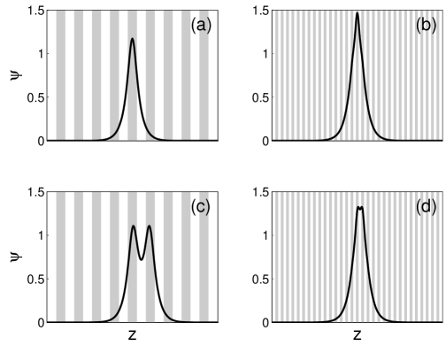
Figure 1: Profiles of on-site and off-site solitary waves in the nonlinear lattice equation (2.5) at two values of $\epsilon=0.5$ and $0.15$ (with $\mu=1$). Upper row: on-site solutions; lower row: off-site solutions; left column: $\epsilon=0.5$; right column: $\epsilon=0.15$. The vertical stripes mark locations of high nonlinear-lattice values.

Next we numerically determine the linear stability of these solitary waves and make a comparison with our analytical results. The whole linear-stability spectra for the on-site and off-site solitary waves in Fig. 1(b,d) at $\epsilon=0.15$ are shown in Fig. 2(a,b). The spectrum in Fig. 2(a) lies entirely on the imaginary axis, indicating that this on-site solitary wave is linearly stable. In this spectrum, a pair of purely imaginary discrete eigenvalues can be seen. These are the counterparts of our analytical imaginary eigenvalues given by Eq. (5.21) with $x_{0s}=\theta/\kappa_{0}=0$. The spectrum in Fig. 2(b) contains a real positive eigenvalue, indicating that the underlying off-site solitary wave is linearly unstable, in agreement with our analytical prediction. In particular, this positive eigenvalue is the counterpart of our analytical positive eigenvalue given by Eq. (5.21) with $x_{0s}=(\theta+\pi)/\kappa_{0}=\pi$.

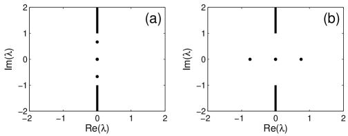
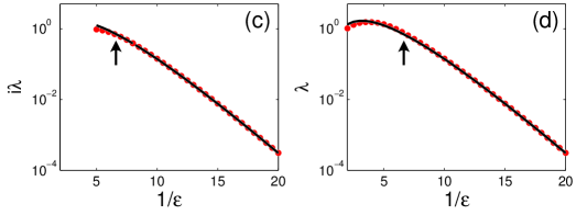
Figure 2: (a,b) Stability spectra for the on-site and off-site solitary waves in Fig. 1(b,d) respectively ($\epsilon=0.15$); (c,d) comparison between numerical and analytical discrete eigenvalues of on-site and off-site solitary waves at various values of $\epsilon$; dotted lines: numerical values; solid lines: analytical values from formulae (5.21). The arrows mark locations of the value of $\epsilon$ in (a,b).

Now we quantitatively compare the numerical linear-stability eigenvalues with the analytical formula (5.21). For this purpose, we have numerically obtained the discrete eigenvalues (as those in Fig. 2(a,b)) for on-site and off-site solitary waves at various values of $\epsilon$, and the results are shown in Fig. 2(c,d) by dotted lines. The analytical eigenvalues from the formulae (5.21) for the on-site and off-site cases are also plotted as solid lines, and excellent agreement can be seen for both cases. This verifies that the analytical formula (5.21) is asymptotically accurate.

Finally, we numerically examine how these solitary waves evolve nonlinearly under weak perturbations. For this purpose, we again consider the on-site and off-site solitary waves in Fig. 1(b,d) at $\epsilon=0.15$. We perturb these waves initially by a small phase gradient as

$$\Psi(z,0)=\psi(z)e^{i\gamma z},$$ (6.3)

where $\psi(z)$ is the solitary wave and $\gamma=0.01$. This phase-gradient perturbation gives the solitary wave a small initial ‘push’. Evolutions of the on-site and off-site solitary waves under this perturbation are obtained by simulating Eq. (2.1) with the above initial condition (6.3), and the results are displayed in Fig. 3. It is seen that the on-site solitary wave is not affected by this perturbation and stays at its initial on-site position (see Fig. 3(a)), consistent with the linear stability of this on-site solitary wave established in Fig. 2(a). On the other hand, under the same perturbation, the off-site solitary wave moves from its initial off-site position to a nearby on-site position and then oscillates around it (see Fig. 3(b)). When $t\to\infty$, the oscillation eventually dies out, and the solution evolves into a stationary on-site solitary wave. This nonlinear evolution scenario is consistent with the linear instability of this off-site solitary wave, as shown in Fig. 2(b).

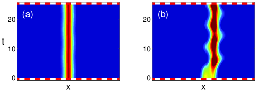
Figure 3: Nonlinear evolutions of the on-site (a) and off-site (b) solitary waves in Fig. 1(b,d) under phase-gradient perturbations (6.3). Red bars represent locations of high nonlinear-lattice values.

7 Bound states

In addition to the two fundamental solitary waves obtained earlier, the nonlinear-lattice equation (2.5) also admits higher-order solitary waves, or bound states [17]. These can be analytically constructed by matching the tails of more than one of the nonlocal solitary waves discussed in Sec. 4. A similar construction has been detailed in [25] for bound states of the NLS equation with a linear sinusoidal periodic potential (see also [26]). Here we shall sketch the analysis for bound states involving two nonlocal solitary waves in a nonlinear lattice.

For simplicity, we assume the symmetric cosine nonlinear lattice (6.1), with given depth $g_{0}$. In this case, $\kappa_{0}=1$ and $\theta=0$. Then we consider two nonlocal solitary waves of (see Sec. 4), $\psi^{+}(z)$ and $\psi^{-}(z)$, whose main ‘sech’ humps are centered at $z_{0}^{+}=\epsilon x_{0}^{+}$ and $z_{0}^{-}=-\epsilon x_{0}^{-}$, respectively, with $z_{0}^{\pm}>0$, and $z_{0}^{+}+z_{0}^{-}\gg 1$ (large separation). In addition, let $\psi^{\pm}(z)\to 0$ as $z\to\pm\infty$, so that the right-hand tail of $\psi^{-}(z)$ and the left-hand tail of $\psi^{+}(z)$ are nonlocal. According to (4.26), the right-hand tail of $\psi^{-}(z)$ is given by

$$\psi^{-}(z)\sim 2a{\rm e}^{-(z+z_{0}^{-})/\beta}-{4\pi\beta^{3}\widehat{C}\over\epsilon^{4}}{\rm e}^{-\pi\beta/2\epsilon}\sin x_{0}^{-}\ {\rm e}^{(z+z_{0}^{-})/\beta}\qquad(z\gg-z_{0}^{-})\,.$$ (7.1)

For symmetric lattice functions $g(x)$, Eq. (2.5) is invariant with respect to reflection in $z$ ($z\to-z$). In addition, if $\psi(z)$ is a solution to (2.5), so is $-\psi(z)$. Thus the left-hand tail of $\psi^{+}(z)$ can be obtained from (4.26) after reflection in $z$ as

$$\psi^{+}(z)\sim\pm 2a{\rm e}^{(z-z_{0}^{+})/\beta}\mp{4\pi\beta^{3}\widehat{C}\over\epsilon^{4}}{\rm e}^{-\pi\beta/2\epsilon}\sin x_{0}^{+}\ {\rm e}^{-(z-z_{0}^{+})/\beta}\qquad(z\ll z_{0}^{+})\,.$$ (7.2)

Here, the upper sign in (7.2) corresponds to the case where the main humps of the two nonlocal waves have the same polarity (sign), while the lower sign pertains to the case of opposite polarity. To obtain a solitary wave (bound state) comprising these two nonlocal waves, we require that the right-hand tail (7.1) of $\psi^{-}(z)$ and the left-hand tail (7.2) of $\psi^{+}(z)$ match smoothly in the overlap region $-z_{0}^{-}\ll z\ll z_{0}^{+}$. This requirement gives

$$\sin x_{0}^{-}=\sin x_{0}^{+}=\mp{a\over 2\pi\widehat{C}}{\epsilon^{4}\over\beta^{3}}{\rm e}^{\pi\beta/2\epsilon}\,{\rm e}^{-\epsilon(x_{0}^{+}+x_{0}^{-})/\beta}\,.$$ (7.3)

These matching equations are identical to those in [25] after a scaling in $(x_{0}^{-},x_{0}^{+},\epsilon,\widehat{C})$, and their solutions can be taken directly from [25]. Specifically, for fixed $\mu>0$, $\epsilon>0$ and given sign (polarity), these equations admit an infinite number of solutions $(x_{0}^{-},x_{0}^{+})$. Each solution corresponds to a bound state whose leading-order approximation is

$$\psi(z)\sim a\mathop{\rm sech}\nolimits{z+z_{0}^{-}\over\beta}\pm a\mathop{\rm sech}\nolimits{z-z_{0}^{+}\over\beta},$$ (7.4)

and a continuous family of bound states is obtained when $\epsilon$ or $\mu$ varies. Each bound-state family contains triple branches and, for fixed $\epsilon$, these branches disappear when $\mu$ falls below a certain threshold (or equivalently, for fixed $\mu$, these branches disappear when $\epsilon$ falls below a certain threshold). To demonstrate, we take the cosine nonlinear potential (6.1) with $g_{0}=1$ and $\epsilon=0.15$. In this nonlinear lattice, a family of bound states comprising two fundamental solitons of the same polarity is numerically obtained and displayed in Fig. 4. The power curve $P(\mu)$ of this family, defined as

$$P(\mu)=\int_{-\infty}^{\infty}\psi^{2}(z;\mu)\hskip 1.9919ptdz,$$ (7.5)

contains three branches. On the lower branch, the bound state comprises two on-site fundamental solitons which are separated approximately by 8 lattice sites. On the upper branch, the bound state comprises two off-site fundamental solitons which are separated approximately by 7 lattice sites. On the middle branch, the bound state comprises an on-site and an off-site fundamental soliton which are separated approximately by 7.5 lattice sites. These solution branches exist only when $\mu>\mu_{c}\approx 0.7887$; thus, they do not bifurcate from infinitesimal linear waves at the edge $\mu=0$ of the continuous spectrum of Eq. (2.1). These numerical results are in good agreement with the theoretical predictions based on the formulae (7.3)–(7.4).

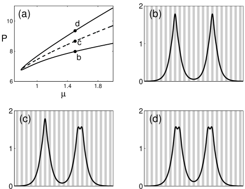
Figure 4: A family of bound states with same polarity in Eq. (2.5) for the cosine nonlinear potential (6.1) with $g_{0}=1$ and $\epsilon=0.15$: (a) the power curve; (b,c,d) bound-state profiles at points of the power branches marked by the same letters in (a).

8 Concluding remarks

In this article, we developed an asymptotic theory for long solitary waves and their linear stability in a general nonlinear lattice. Based on exponential asymptotics, we showed that long solitary waves can only be located at two positions relative to the nonlinear lattice, regardless of the number of local maxima and minima in the lattice. In general, these positions are determined by a certain recurrence relation that includes information beyond all orders of the usual multiple-scale perturbation expansion. From the same recurrence relation, one may also deduce that, of these two solitary waves, one is linearly stable and the other is unstable. If the lattice is symmetric, then the solitary-wave positions are simply the point of symmetry and half a lattice-period away from it. In particular, for the special cosine lattice, the solitary wave centered at the maximum/minimum of the lattice is linearly stable/unstable. We also derived an analytical formula for the linear-stability eigenvalues, which are exponentially small with respect to the long-wave parameter (the ratio between the lattice period and the width of the solitary wave). The predictions of this analytical formula were compared against numerical results and excellent agreement was observed. Finally, it was pointed out that an infinite number of multi-solitary-wave bound states are possible in a nonlinear lattice, and their analytical construction was presented.

The exponential asymptotics procedure used in this investigation closely resembles that in [24, 25] for linear lattices and in [26, 27] for the fifth-order KdV equation. In fact, the integral equation (4.18), which plays a key role in the analysis, actually arises in all these three different physical models. This suggests that our asymptotic procedure in the wavenumber domain is a possibly universal treatment of multiscale solitary-wave problems, and it is likely to find applications in other physical settings as well.

References

- [1] O
- [2] D.J. BENNEY and A.C. NEWELL, Nonlinear wave envelopes, J. Math. Phys. 46: 133–139 (1967).
- [3] A.D.D. CRAIK, Wave Interactions and Fluid Flows (Cambridge UP, Cambridge, 1985).
- [4] M.J. ABLOWITZ and H. SEGUR, Solitons and the Inverse Scattering Transform (SIAM, Philadelphia, 1981).
- [5] F. DALFOVO, S. GIORGINI, L.P. PITAEVSKII and S. STRINGARI, Theory of Bose–Einstein condensation in trapped gases, Rev. Mod. Phys. 71: 463–512 (1999).
- [6] Y.S. KIVSHAR and G.P. AGRAWAL, Optical Solitons: From Fibers to Photonic Crystals (Academic Press, San Diego, 2003).
- [7] J. YANG, Nonlinear Waves in Integrable and Nonintegrable Systems (SIAM, Philadelphia, 2010).
- [8] D.N. CHRISTODOULIDES, F. LEDERER and Y. SILBERBERG, Discretizing light behaviour in linear and nonlinear waveguide lattices, Nature 424: 817–823 (2003).
- [9] O. MORSCH and M.K. OBERTHALER, Dynamics of Bose–Einstein condensates in optical lattices, Rev. Mod. Phys. 78: 179–215 (2006).
- [10] P.G. KEVREKIDIS, D.J. FRANTZESKAKIS, and R. CARRETERO-GONZALEZ (Eds.), Emergent Nonlinear Phenomena in Bose–Einstein Condensates: Theory and Experiment (Springer, Berlin, 2007).
- [11] M. SKOROBOGATIY and J. YANG, Fundamentals of Photonic Crystal Guiding (Cambridge University Press, Cambridge, 2009).
- [12] J.W. FLEISCHER, M. SEGEV, N.K. EFREMIDIS, and D.N. CHRISTODOULIDES, Observation of two-dimensional discrete solitons in optically induced nonlinear photonic lattices, Nature 422: 147–150 (2003).
- [13] D. BLÖMER, A. SZAMEIT, F. DREISOW, T. SCHREIBER, S. NOLTE, and A. TÜNNERMANN, Nonlinear refractive index of fs-laser-written waveguides in fused silica, Opt. Express 14: 2151-2157 (2006).
- [14] S. INOUYE, M.R. ANDREW, J. STENGER, H.J. MIESNER, D.M. STAMPER-KURN and W. KETTERLE, Observation of Feshbach resonances in a Bose–Einstein condensate, Nature 392: 151–154 (1998).
- [15] M. THEIS, G. THALHAMMER, K. WINKLER, M. HELLWIG, G. RUFF, R. GRIMM and J.H. DENSCHLAG, Tuning the scattering length with an optically induced Feshbach resonance, Phys. Rev. Lett. 93:123001 (2004).
- [16] R. YAMAZAKI, S. TAIE, S. SUGAWA and Y. TAKAHASHI, Submicron spatial modulation of an interatomic interaction in a Bose–Einstein condensate, Phys. Rev. Lett. 105:050405 (2010).
- [17] H. SAKAGUCHI and B.A. MALOMED, Matter-wave solitons in nonlinear optical lattices, Phys. Rev. E 72:046610 (2005).
- [18] G. FIBICH, Y. SIVAN and M.I. WEINSTEIN, Bound states of nonlinear Schrödinger equations with a periodic nonlinear microstructure, Physica D 217: 31–57 (2006).
- [19] A.S. RODRIGUES, P.G. KEVREKIDIS, M.A. PORTER, D.J. FRANTZESKAKIS, P. SCHMELCHER and A.R. BISHOP, Matter-wave solitons with a periodic, piecewise-constant scattering length, Phys. Rev. A 78:013611 (2008).
- [20] M.A. PORTER, P.G. KEVREKIDIS, B.A. MALOMED, and D.J. FRANTZESKAKIS, Modulated amplitude waves in collisionally inhomogeneous Bose–Einstein condensates, Physica D 229: 104–115 (2007).
- [21] J. BELMONTE-BEITIA, V.M. PÉREZ-GARCÍA, V. VEKSLERCHIK and P.J. TORRES, Lie symmetries and solitons in nonlinear systems with spatially inhomogeneous nonlinearities, Phys. Rev. Lett. 98: 064102 (2007).
- [22] J. BELMONTE-BEITIA and D.E. PELINOVSKY, Bifurcation of gap solitons in periodic potentials with a periodic sign-varying nonlinearity coefficient, Applicable Analysis 89: 1335–1350 (2010).
- [23] Y. SIVAN, G. FIBICH and M.I. WEINSTEIN, Waves in nonlinear lattices: Ultrashort optical pulses and Bose–Einstein condensates, Phys. Rev. Lett. 97:193902 (2006).
- [24] G. HWANG, T.R. AKYLAS and J. YANG, Gap solitons and their linear stability in one-dimensional periodic media, Physica D 240: 1055 -1068 (2011).
- [25] T.R. AKYLAS, G. HWANG and J. YANG, From nonlocal gap solitary waves to bound states in periodic media, submitted.
- [26] T.S. YANG and T.R. AKYLAS, On asymmetric gravity-capillary solitary waves, J. Fluid Mech. 330: 215–232 (1997).
- [27] D.C. CALVO, T.S. YANG and T.R. AKYLAS, On the stability of solitary waves with decaying oscillatory tails, Proc. R. Soc. Lond. A. 456: 469–487 (2000).
- [28] D.E. PELINOVSKY, A.A. SUKHORUKOV and Y.S. KIVSHAR, Bifurcations and stability of gap solitons in periodic potentials, Phys. Rev. E 70:036618 (2004).
UNIVERSITY OF VERMONT
MASSACHUSETTS INSTITUTE OF TECHNOLOGY
UNIVERSITY OF VERMONT
(Received June 24, 2011)