A 10	Monte Carlo Simulations
	Michael Bachmann
	Institut für Festkörperforschung (IFF-2) and Institute for Advanced Simulation (IAS-2)
	Forschungszentrum Jülich, D-52425 Jülich, Germany

1 Introduction

For a system under thermal conditions in a heat bath with temperature $T$, the dynamics of each of the system particles is influenced by interactions with the heat-bath particles. If quantum effects are negligible (what we will assume in the following), the classical motion of any system particle looks erratic; the particle follows a stochastic path. The system can “gain” energy from the heat bath by these collisions (which are typically more generally called “thermal fluctuations”) or “lose” energy by friction effects (dissipation). The total energy of the coupled system of heat bath and particles is a conserved quantity, i.e., fluctuation and dissipation refer to the energetic exchange between heat bath and system particles only. Consequently, the coupled system is represented by a microcanonical ensemble, whereas the particle system is in this case represented by a canonical ensemble: The energy of the particle system is not a constant of motion. Provided heat bath and system are in thermal equilibrium, i.e., heat-bath and system temperature are identical, fluctuations and dissipation balance each other. This is the essence of the celebrated fluctuation-dissipation theorem [1]. In equilibrium, only the statistical mean of the particle system energy is constant in time.

This canonical behavior of the system particles is not accounted for by standard Newtonian dynamics (where the system energy is considered to be a constant of motion). In order to perform molecular dynamics (MD) simulations of the system under the influence of thermal fluctuations, the coupling of the system to the heat bath is required. This is provided by a thermostat, i.e., by extending the equations of motion by additional heat-bath coupling degrees of freedom [2]. The introduction of thermostats into the dynamics is a notorious problem in MD and it cannot be considered to be solved satisfactorily to date [3]. In order to take into consideration the stochastic nature of any particle trajectory in the heat bath, a typical approach is to introduce random forces into the dynamics. These forces represent the collisions of system and heat-bath particles on the basis of the fluctuation-dissipation theorem [1].

Unfortunately, MD simulations of complex systems on microscopic and mesoscopic scales are extremely slow, even on the largest available computers. A prominent example is the folding of proteins with natural time scales of milliseconds to seconds. It is currently still impossible to simulate folding events of bioproteins under realistic conditions, since even longest MD runs are hardly capable of generating single trajectories of more than a few microseconds. Consequently, if the intrinsic time scale of a realistic model exceeds the time scale of an MD simulation of this model, MD cannot seriously be applied in these cases.

However, many interesting questions do not require to consider the intrinsic dynamics of the system explicitly. This regards, e.g., equilibrium thermodynamics, which includes all relevant phenomena of cooperativity – the collective original source for the occurrence of phase transitions. Stability of all matter, independently whether soft or solid, requires fundamental ordering principles. We are far away from having understood the general physical properties of transition processes that separate, e.g., ordered and disordered phases, crystals and liquids, glassy and globular polymers, native and intermediate protein folds, ferromagnetic and paramagnetic states of metals, Bose-Einstein condensates and bosonic gases, etc. Meanwhile, the history of research of collective or critical phenomena has already lasted for more than hundred years and the universality hypothesis has already been known for several decades [4]. Though, no complete theory exists which is capable relating to each other phenomena such as protein folding (unfolding) and freezing (melting) of solid matter. The reason is that the first process is dominated by finite-size effects, whereas the latter seems to be a macroscopic “bulk” phenomenon. However, although doubtlessly associated to different length scales which differ by orders of magnitude, both examples are based on cooperativity, i.e., the collective multi-body interplay of a large number of atoms. Precise theoretical analyses are extremely difficult, even more, if several attractive and repulsive interactions compete with each other and if the system does not possess any obvious internal symmetries (which is particularly apparent for “glassy” heteropolymers like proteins). On the experimental side, the situation has not been much better as the resolution of the data often did not allow an in-depth analysis of the simultaneous microscopic effects accompanying cooperative phenomena. This has dramatically improved by novel experimental techniques enabling to measure the response of the system to local manipulations, giving insight in the mesoscopic and macroscopic multi-body effects upon activation. On the other hand, a systematic understanding requires a theoretical basis. The relevant physical forces have been known for a long time, but the efficient combination of technical and algorithmic prerequisites has been missing until recently. The general understanding of cooperativity in complex systems as a statistical effect, governed by a multitude of forces acting on different energy and length scales, requires the study of the interplay of entropy and energy. The key to this is currently only provided by Monte Carlo computer simulations [5].

2 Conventional Markov-chain Monte Carlo sampling

2.1 Ergodicity and finite time series

The general idea behind all Monte Carlo methodologies is to provide an efficient stochastic sampling of the configurational or conformational phase space or parts of it with the objective to obtain reasonable approximations for statistical quantities such as expectation values, probabilities, fluctuations, correlation functions, densities of states, etc.

A given system conformation (e.g., the geometric structure of a molecule) ${\bf X}$ is locally or globally modified to yield a conformation ${\bf X}^{\prime}$. This update or “move” is then accepted with the transition probability $t({\bf X}\to{\bf X}^{\prime})$. Frequently used updates for polymer models are, for example, random translational changes of single monomer positions, bond angle modifications, or rotations about covalent bond axes. More global updates consist of combined local updates, which can be necessary to satisfy constraints such as fixed bond lengths or simply to improve efficiency. It is, however, a necessary condition for correct statistical sampling that Monte Carlo moves are ergodic, i.e., the chosen set of moves must, in principle, guarantee to reach any conformation out of any other conformation. Since this is often hard to prove and an insufficient choice of move sets can result in systematic errors, great care must be dedicated to choose appropriate moves or sets of moves. Since molecular models often contain constraints, the construction of global moves can be demanding. Therefore, reasonable and efficient moves have to be chosen in correspondence to the model of a system to be simulated.

A Monte Carlo update corresponds to the discrete “time step” $\Delta\tau_{0}$ in the simulation process. In order to reduce correlations, typically a number of updates is performed between measurements of a quantity $O$. This series of updates is called a “sweep” and the “time” passed in a single sweep is $\Delta\tau=N\Delta\tau_{0}$ if the sweep consists of $N$ updates. Thus, if $M$ sweeps are performed, the discrete “time series” is expressed by the vector $(O(\tau_{\text{init}}+\Delta\tau),O(\tau_{\text{init}}+2\Delta\tau),\ldots,O(\tau_{\text{init}}+m\Delta\tau),\ldots,O(\tau_{\text{init}}+M\Delta\tau))$ and represents the Monte Carlo trajectory. The period of equilibration $\tau_{\text{init}}$ sets the starting point of the measurement. For convenience, we use the abbreviation $O_{m}\equiv O(\tau_{\text{init}}+m\Delta\tau)$ and $\tau_{m}=\tau_{\text{init}}+m\Delta\tau$ with $m=1,2,\ldots,M$ in the following.

According to the theory of ergodicity, averaging a quantity over an infinitely long time series is identical to perform the statistical ensemble average:

$$\overline{O}=\lim_{M\to\infty}\frac{1}{M}\sum\limits_{m=1}^{M}O_{m}\equiv\langle O\rangle=\int{\cal D}XO(\textbf{X})p(\textbf{X}),$$ (1)

where ${\cal D}X$ represents the formal integral measure for the infinitesimal scan of the conformation space and $p({\bf X})$ is the energy dependent microstate probability of the conformation X in the relevant ensemble in thermodynamic equilibrium [in the canonical ensemble with temperature $T$, simply $p({\bf X})=\exp[-E({\bf X})/k_{\text{B}}T]$]. This is the formal basis for Monte Carlo sampling. However, only finite time series can be simulated on a computer. For a finite number of sweeps $M$ in a sample $k$, the relation (1) can only be satisfied approximately, $M^{-1}\sum_{m=1}^{M}O^{(k)}_{m}=\overline{O}^{(k)}\approx\langle O\rangle$. Note that the mean value $\overline{O}^{(k)}$ will depend on the sample $k$, meaning that it is likely that another sample $k^{\prime}$ will yield a different value $\overline{O}^{(k^{\prime})}\neq\overline{O}^{(k)}$. In order to define a reasonable estimate for the statistical error, it is necessary to start from the assumption that we have generated an infinite number of independent samples $k$. In this case the distribution of the estimates $\overline{O}^{(k)}$ is Gaussian, according to the central limit theorem of uncorrelated samples. The exact average of the estimates is then given by $\langle\overline{O}\rangle$. The statistical error of $\overline{O}$ is thus suitably defined as the standard deviation of the Gaussian:

$$\varepsilon_{\overline{O}}=\sqrt{\left\langle\left(\overline{O}-\langle\overline{O}\rangle\right)^{2}\right\rangle}=\sqrt{\langle\overline{O}^{2}\rangle-\langle\overline{O}\rangle^{2}}=\sqrt{\frac{1}{M^{2}}\sum\limits_{m=1}^{M}\sum\limits_{n=1}^{M}A_{mn}\sigma^{2}_{O_{m}}},$$ (2)

where

$$A_{mn}=\frac{\langle O_{m}O_{n}\rangle-\langle O_{m}\rangle\langle O_{n}\rangle}{\langle O_{m}^{2}\rangle-\langle O_{m}\rangle^{2}}$$ (3)

is the autocorrelation function and $\sigma^{2}_{O_{m}}=\langle O_{m}^{2}\rangle-\langle O_{m}\rangle^{2}$ is the variance of the distribution of individual data $O_{m}$. If the Monte Carlo updates in each sample are performed completely randomly without memory, i.e., a new conformation is created independently of the one in the step before (which is a possible but typically very inefficient strategy), two measured values $O_{m}$ and $O_{n}$ are uncorrelated, if $m\neq n$. Then, the autocorrelation function simplifies to $A_{mn}=\delta_{mn}$ and the statistical error satisfies the celebrated relation

$$\varepsilon_{\overline{O}}=\frac{\sigma_{O_{m}}}{\sqrt{M}}.$$ (4)

Since the exact distribution of $O_{m}$ values and the “true” expectation value $\langle O\rangle$ are unchanged in the simulation (but unfortunately unknown), the standard deviation $\sigma_{O_{m}}$ is constant, too. Thus, the statistical error decreases with $1/\sqrt{M}$.

In practice, most of the efficient Monte Carlo techniques generate correlated data, in which case we have to fall back to the more general formula (2). It can conveniently be rewritten as

$$\varepsilon_{\overline{O}}=\sigma_{O_{m}}/{\sqrt{M_{\text{eff}}}}$$ (5)

with the effective statistics $M_{\text{eff}}=M/\Delta\tau_{\text{ac}}\leq M$, where $\Delta\tau_{\text{ac}}$ corresponds to the autocorrelation time. This means, the statistics is effectively reduced by the number of sweeps until the correlations have decayed. Since it takes at least the time $\Delta\tau_{\text{ac}}=N_{\text{ac}}\Delta\tau_{0}$ to generate statistically independent conformations, a sweep can simply contain as many updates $N_{\rm ac}$ as necessary to satisfy $\Delta\tau\approx\Delta\tau_{\text{ac}}$ without losing effective statistics. In this case, the $M\approx M_{\text{eff}}$ data entering into the effective statistics are virtually uncorrelated. This is also the general idea behind advanced, computationally convenient error estimation methods such as binning and jackknife analyses [7, 6]. For the correctness of the measurements, $M\approx M_{\text{eff}}$ is not a necessary condition; more sweeps with less updates in each sweep, i.e., periods between measurements shorter than $\Delta\tau_{\text{ac}}$ only yield redundant statistical information. This is not even wrong, but computationally inefficient as it does not improve the statistical error (5).

2.2 Master equation

Beside ergodicity, another demand for correct statistical sampling is to ensure that the probability distribution $p({\bf X})$ associated to the desired statistical ensemble is independent of time. This can only be achieved in the simulation, if the relevant part of the phase space is sampled sufficiently efficient to allow for quick convergence towards a stable or, more precisely, stationary estimate for $p({\bf X})$. In most of the Monte Carlo methods, the simulation follows a Markov dynamics, i.e., the update of a given conformation ${\bf X}$ to a new one ${\bf X}^{\prime}$ is not influenced by the history that led to ${\bf X}$, i.e., the dynamics does not possess an explicit memory. Such a Markov process can be described by the master equation:

$$\frac{\Delta p({\bf X})}{\Delta\tau_{0}}=\sum\limits_{{\bf X}^{\prime}}[p({\bf X}^{\prime})t({\bf X}^{\prime}\to{\bf X};\Delta\tau_{0})-p({\bf X})t({\bf X}\to{\bf X}^{\prime};\Delta\tau_{0})],$$ (6)

where $t({\bf X}\to{\bf X}^{\prime};\Delta\tau_{0})$ is the transition probability from ${\bf X}$ to ${\bf X}^{\prime}$ in a single update (or “time” step $\Delta\tau_{0}$). Due to particle conservation, it satisfies the normalization condition $\sum_{{\bf X}^{\prime}}t({\bf X}\to{\bf X}^{\prime};\Delta\tau_{0})=1$, i.e., whatever update we perform, we must end up with a state ${\bf X}^{\prime}$ which is an element of the conformational space. The condition $\Delta p({\bf X})/\Delta\tau_{0}=0$ ensures that the ensemble is in a stationary state if the right-hand side of Eq. (6) vanishes. Since the stationarity condition also allows solutions where the distribution function $p({\bf X})$ dynamically changes on cycles which, however, is not the physical situation in a statistical equilibrium ensemble, we demand more rigorously that the expression in the brackets vanishes. This is called the detailed balance condition. Consequently, the ratio of transition rates is given by

$$\frac{t({\bf X}\to{\bf X}^{\prime};\Delta\tau_{0})}{t({\bf X}^{\prime}\to{\bf X};\Delta\tau_{0})}=\frac{p({\bf X}^{\prime})}{p({\bf X})}$$ (7)

and thus independent of the length of “time” step $\Delta\tau_{0}$, which we, therefore, omit in the following. From this relation, it follows that it is obviously a good idea to construct an efficient Markov chain Monte Carlo algorithm, i.e., to choose appropriate acceptance probabilities for the Monte Carlo updates to yield the correct transition probability $t({\bf X}\to{\bf X}^{\prime})$, by taking into account the basic microstate probabilities of the statistical ensemble to be simulated. Markov Monte Carlo simulations in the canonical ensemble at fixed temperature $T$, for example, have to satisfy

$$\frac{t({\bf X}\to{\bf X}^{\prime})}{t({\bf X}^{\prime}\to{\bf X})}=e^{-\beta\Delta E},$$ (8)

where $\Delta E=E({\bf X}^{\prime})-E({\bf X})$ is the energy difference between the new and the old state. Thus, the transition rate to reach a state ${\bf X}^{\prime}$, supposed to be energetically favored if compared with the initial state ${\bf X}$, grows exponentially with $\Delta E<0$. “Climbing the hill” towards a state with higher energy ($\Delta E>0$) is, on the other hand, exponentially suppressed. This is in correspondence with the interpretation of the Markov transition state theory. Hence, it is possible to study the kinetic behavior (identification of free-energy barriers, measuring the height of barriers, estimating transition rates, etc.) of a series of processes in equilibrium – for example the folding and unfolding behavior of a protein – by means of Monte Carlo simulations. To quantify the dynamics of a process, i.e., the explicit time dependence is, however, less meaningful as the conformational change in a single time step depends on the move set and does not follow a physical, e.g., Newtonian, dynamics.

2.3 Selection and acceptance probabilities

In order to correctly satisfy the detailed balance condition (7) in a Monte Carlo simulation, we have to take into account that each Monte Carlo step consists of two parts. First, a Monte Carlo update of the current state is suggested and second, it has to be decided whether or not to accept it according to the chosen sampling strategy. In fact, both steps are independent of each other in the sense that each possible update can be combined with any sampling method. Therefore, it is useful to factorize the transition probability $t({\bf X}\to{\bf X}^{\prime})$ in the selection probability $s({\bf X}\to{\bf X}^{\prime})$ for a desired update from ${\bf X}$ to ${\bf X}^{\prime}$ and the acceptance probability $a({\bf X}\to{\bf X}^{\prime})$ for this update:

$$t({\bf X}\to{\bf X}^{\prime})=s({\bf X}\to{\bf X}^{\prime})a({\bf X}\to{\bf X}^{\prime}).$$ (9)

The acceptance probability is typically used in the form

$$a({\bf X}\to{\bf X}^{\prime})=\min\left(1,\sigma({\bf X},{\bf X^{\prime}})w({\bf X}\to{\bf X}^{\prime})\right),$$ (10)

with the ratio of microstate probabilities

$$w({\bf X}\to{\bf X}^{\prime})=\frac{p({\bf X^{\prime}})}{p({\bf X})}$$ (11)

and the ratio of forward and backward selection probabilities

$$\sigma({\bf X},{\bf X}^{\prime})=\frac{s({\bf X}^{\prime}\to{\bf X})}{s({\bf X}\to{\bf X}^{\prime})}.$$ (12)

The expression (10) for the acceptance probability naturally fulfills the detailed-balance condition (7). The selection ratio $\sigma({\bf X},{\bf X}^{\prime})$ is unity, if the forward and backward selection probabilities are identical. This is typically the case for “simple” local Monte Carlo updates. If, for example, the update is a translation of a coordinate, $x^{\prime}=x+\Delta x$, where $\Delta x\in[-x_{0},+x_{0}]$ is chosen from a uniform random distribution, the forward selection for a translation by $\Delta x$ is equally probable to the backward move, i.e., to translate the particle by $-\Delta x$. This is also valid for rotations about bonds in a molecular system such as rotations about dihedral angles in a protein. If selection probabilities for forward and backward moves differ, the selection rate is not unity. This is often the case in complex, global updates which comprise several steps. Then, the determination of the correct selection probabilities can be difficult and the selection rate has typically to be estimated in test runs first. To this class of updates belong the biased Gaussian steps [8], where a series of torsional updates of a few sequential protein backbone dihedral angles are performed in order to ensure that the update does not drastically change the protein conformation (which would likely be rejected).

Note that the overall efficiency of a Monte Carlo simulation depends on both, a model-specific choice of a suitable set of moves and an efficient microstate sampling strategy based on $w({\bf X}\to{\bf X}^{\prime})$.

2.4 Simple sampling

The choice of the microstate probabilities $p({\bf X})$ is not necessarily coupled to a certain physical statistical ensemble. Thus, the simplest choice is a uniform probability $p({\bf X})=1$ independently of ensemble-specific microstate properties. Thus also $w({\bf X}\to{\bf X}^{\prime})=1$ and if the Monte Carlo updates satisfy $\sigma({\bf X},{\bf X}^{\prime})=1$, the acceptance probability is trivially also unity, $a({\bf X}\to{\bf X}^{\prime})=1$, i.e., all generated Monte Carlo updates are accepted, independently of the type of the update. Thus, updates of system degrees of freedom can be performed randomly, where the random numbers are chosen from a uniform distribution. This method is called simple sampling. However, its applicability is quite limited. Consider, for example, the estimation of the density of states for a discrete system with this method. After having performed a series of $M$ updates, we will have obtained an energetic histogram $h(E)=M^{-1}\sum_{m=1}^{M}\delta_{E_{m},E}$ which represents an estimate for the density of states. The canonical expectation value of the energy can be estimated by $\overline{E}=M^{-1}\sum_{m=1}^{M}E_{m}e^{-E_{m}/k_{\text{B}}T}=\sum_{E}Eh(E)e^{-E/k_{\text{B}}T}$. If the microstates are generated randomly from a uniform distribution, it is obvious that we will sample the states ${\bf X}$ with an energy $E({\bf X})$ in accordance with their system-specific frequency or degeneracy. High-frequency states thermodynamically dominate in the purely disordered phase. However, near phase transitions towards more ordered phases, the density of states drops rapidly – typically by many orders of magnitude. The degeneracies of the lowest-energy states representing the most ordered states are so small that the thermodynamically most interesting transition region spans even in rather small systems often hundreds to thousands orders of magnitude.

To bridge a region of 100 orders of magnitude between an ordered and a disordered phase by simple sampling would roughly mean to perform about 10${}^{\text{100}}$ updates in order to find a single ordered state. Assuming that a simple single update would require only a few CPU operations, it will at least take 1 ns on standard CPU cores. Even under this optimistic assumption, it would take more than 10${}^{\text{83}}$ years to perform 10${}^{\text{100}}$ updates on a single core! Thus, for studies of complex systems with sufficiently many degrees of freedom allowing for cooperativity, simple sampling is of very little use.

2.5 Metropolis sampling

Because of the dominance of a certain restricted space of microstates in ordered phases, it is obviously a good idea to primarily concentrate in a simulation on a precise sampling of the microstates that form the macrostate under given external parameters such as, for example, the temperature. The canonical probability distribution functions clearly show that within the certain stable phases, only a limited energetic space of microstates is noticeably populated, whereas the probability densities drop off rapidly in the tails. Thus, an efficient sampling of this state space should yield the relevant information within comparatively short Markov chain Monte Carlo runs. This strategy is called importance sampling.

The standard importance sampling variant is the Metropolis method [9], where the algorithmic microstate probability $p({\bf X})$ is identified with the canonical microstate probability $p({\bf X})\sim e^{-\beta E({\bf X})}$ at the given temperature $T$ ($\beta=1/k_{\text{B}}T$). Thus, the acceptance probability (10) is governed by the ratio of the canonical thermal weights of the microstates:

$$w({\bf X}\to{\bf X}^{\prime})=e^{-\beta[E({\bf X}^{\prime})-E({\bf X})]}.$$ (13)

According to Eq. (10), a Monte Carlo update from ${\bf X}$ to ${\bf X}^{\prime}$ (assuming $\sigma({\bf X},{\bf X}^{\prime})=1$) is accepted, if the energy of the new microstate is lower than before, $E({\bf X}^{\prime})<E({\bf X})$. If this update would provoke an increase of energy, $E({\bf X}^{\prime})>E({\bf X})$, the conformational change is accepted only with the probability $e^{-\beta\Delta E}$, where $\Delta E=E({\bf X}^{\prime})-E({\bf X})$. Technically, in the simulation, a random number $r\in[0,1)$ from a uniform distribution is drawn: If $r\leq e^{-\beta\Delta E}$, the move is still accepted, whereas it is rejected otherwise. Thus, the acceptance probability is exponentially suppressed with $\Delta E$ and the Metropolis simulation yields, at least in principle, a time series which is inherently correctly sampled in accordance with the canonical statistics. The arithmetic mean value of a quantity $O$ over the finite Metropolis time series is already an estimate for the canonical expectation value: $\overline{O}=M^{-1}\sum_{m=1}^{M}O_{m}\approx\langle O\rangle$. In the hypothetical case of an infinitely long simulation ($M\to\infty$), this relation is an exact equality, i.e., the deviation is due to the finiteness of the time series only. However, it is just this restriction to a finite amount of data which limits the quality of Metropolis data. Because of the canonical sampling, reasonable statistics is only obtained in the energetic region which is most dominant for a given temperature, whereas in the tails of the canonical distributions the statistics is rather poor. Thus, there are three physically particularly interesting cases where Metropolis sampling as standalone method is little efficient.

First, for low temperatures, where lowest-energy states dominate, the widths of the canonical distributions are extremely small and since $\beta\sim 1/T$ is very large, energetic “uphill” updates are strongly suppressed by the Boltzmann weight $e^{-\beta\Delta E}\to 0$. That means, once caught in a low-energy state, the simulation freezes and it remains trapped in a low-energy state for a long period.

Second, near a second-order phase transition, the standard deviation $\sigma_{E}=\sqrt{\langle E^{2}\rangle-\langle E\rangle^{2}}$ of the canonical energy distribution function gets very large at the critical temperature $T_{C}$, as it corresponds to the maximum (or, in the thermodynamic limit, the divergence) of the specific $C_{V}=\sigma_{E}^{2}/k_{\text{B}}T^{2}$. Thus, a large energetic space must precisely be sampled (“critical fluctuations”) which requires high statistics. Since in Metropolis dynamics, “uphill moves” with $\Delta E>0$ are only accepted with a reasonable rate, if at the transition point the ratio $\Delta E/k_{\text{B}}T_{C}>0$ is not too large, it can take a long time to reach a high-energy state if starting from the low-energy end. Since near $T_{C}$ the correlation length diverges like $\xi\sim|\tau|^{-\nu}$ [with $\tau=(T-T_{C})/T_{C}$] and the correlation time in the Monte Carlo dynamics behaves like $t_{\text{corr}}\sim|\tau|^{-\nu z}$, the dynamic exponent $z$ allows to compare the efficiencies of different algorithms. The larger the value of $z$, the less efficient is the method. Unfortunately, the standard Metropolis method turns out to be one of the least efficient methods in sampling critical properties of systems exhibiting a second-order phase transition.

The third reason is that the Metropolis method does also perform poorly at first-order phase transitions. In this case, the canonical distribution function is bimodal, i.e., it exhibits two separate peaks with a highly suppressed energetic region in-between, since two phases coexist. For the reasons already outlined, it is extremely unlikely to succeed if trying to “jump” from the low- to the high-energy phase by means of Metropolis sampling; it rather would have to explore the valley step by step. Since the energetic region between the phases is entropically suppressed – the number of possible states the system can assume is simply too small – it is thus quite unlikely that this “diffusion process” will lead the system into the high-energy phase, or it will at least take extremely long.

However, apart from lowest-energy and phase transition regions, the Metropolis method can successfully be employed, often in combination with reweighting techniques.

3 Reweighting methods

3.1 Single-histogram reweighting

A standard Metropolis simulation is performed at a given temperature, say $T_{0}$. However, it is often desirable to get also quantitative information about the changes of the thermodynamic behavior at nearby temperatures. Since Metropolis sampling is not a priori restricted to a limited phase space, at least in principle, it is indeed theoretically possible to reweight Metropolis data obtained for a given temperature $T_{0}=1/k_{\text{B}}\beta_{0}$ to a different one, $T=1/k_{\text{B}}\beta$. The idea is to “divide out” the Boltzmann factor $e^{-\beta_{0}E}$ in the estimates for any quantity at the simulation temperature and to multiply it by $e^{-\beta E}$:

$$\langle O\rangle_{T}=\frac{\left\langle Oe^{-(\beta-\beta_{0})E}\right\rangle_{T_{0}}}{\left\langle e^{-(\beta-\beta_{0})E}\right\rangle_{T_{0}}}\approx\overline{O}_{T}=\frac{\sum_{m=1}^{M}O_{m}e^{-(\beta-\beta_{0})E_{m}}}{\sum_{m=1}^{M}e^{-(\beta-\beta_{0})E_{m}}},$$ (14)

where we have again considered that the MC time series of length $M$ is finite. In practice, the applicability of this simple reweighting method is rather limited in case the data series was generated in a single Metropolis run, since the error in the tails of the simulated canonical histograms rapidly increases with the distance from the peak. By reweighting, one of the noisy tails will gain the more statistical weight the larger the difference between the temperatures $T_{0}$ and $T$ is. In combination with the generalized-ensemble methods to be discussed later in this chapter, however, single-histogram reweighting is the only way of extracting the canonical statistics off the simulated histograms and works perfectly.

3.2 Multiple-histogram reweighting

From each Metropolis run, an estimate for the density of states $g(E)$ can easily be calculated. Since the histogram measured in a simulation at temperature $T$, $h(E;T)=\sum_{m=1}^{M}\delta_{E\,E_{m}}$, is an estimate for the canonical distribution function $p_{\text{can}}(E;T)\sim g(E)e^{-\beta E}$, the estimate for the density of states is obtained by reweighting, $\overline{g}(E)=h(E;T)e^{\beta E}$. However, since in a “real” Metropolis run at the single temperature $T$ accurate data can only be obtained in a certain energy interval which depends on $T$, the estimate $\overline{g}(E)$ is restricted to this typically rather narrow energy interval and does by far not cover the whole energetic region reasonably well.

Thus, the question is whether the combination of Metropolis data obtained in simulations at different temperatures, can yield an improved estimate $\overline{g}(E)$. This is indeed possible by means of the multiple-histogram reweighting method [10], sometimes also called “weighted histogram analysis method” (WHAM) [11]. Even though the general idea is simple, the actual implementation is not trivial. The reason is that conventional Monte Carlo simulation techniques such as the Metropolis method cannot yield absolute estimates for the partition sum $Z(T)=\sum_{E}g(E)e^{-\beta E}$, i.e., estimates for the density of states at different energies $g_{i}(E)$ and $g_{j}(E^{\prime})$ can only be related to each other if obtained in the same run, i.e., $i=j$, but not if performed under different conditions. This is not a problem for the estimation of mean values or normalized distribution functions at fixed temperatures as long as the Metropolis data obtained in the respective temperature threads are used, but interpolation to temperatures where no data were explicitly generated, is virtually impossible. Also the multiple-histogram reweighting method does not solve the problem of getting absolute quantities, but at least a “reference partition function” is introduced, which the estimates of the density of states obtained in runs at different simulation temperatures can be related to. Thus, interpolating the data between different temperatures becomes possible.

Basically, the idea is to perform a weighted average of the histograms $h_{i}(E)$, measured in Monte Carlo simulations for different temperatures, i.e., at $\beta_{i}$ (where $i=1,2,\ldots,I$ indexes the simulation thread), in order to obtain an estimator for the density of states by combining the histograms in an optimal way:

$$\hat{g}(E)=\frac{\sum_{i}g_{i}(E)w_{i}(E)}{\sum_{i}w_{i}(E)}.$$ (15)

The exact density of states is given by $g(E)=p_{\text{can}}(E;T)Z(T)e^{\beta E}$ and since the normalized histogram $h_{i}(E)/M_{i}$ obtained in the $i$th simulation thread is an estimator for the canonical distribution function $p_{\text{can}}(E;T_{i})$, the density of states is in this thread estimated by

$$g_{i}(E)=\frac{h_{i}(E)}{M_{i}}Z_{i}e^{\beta_{i}E},$$ (16)

where $Z_{i}$ is the unknown partition function at the $i$th temperature. Since in Metropolis simulations the best-sampled energy region depends on the simulation temperature, the number of histogram entries for a given energy will differ from thread to thread. Thus, the data of the thread with high statistics at $E$ should in this interpolation scheme get more weight than histograms with less entries at $E$. Therefore, the weight shall be controlled by the errors of the individual histograms. A possibility to determine a set of optimal weights is to reduce the deviation of the estimate $\hat{g}(E)$ for the density of states from the unknown exact distribution $\langle g\rangle(E)$, where the symbol $\langle\ldots\rangle$ is used to refer to this quantity as the true distribution which would have been hypothetically obtained in an infinite number of threads (it should not be confused with a statistical ensemble average). As usual, the “best” estimate is the one that minimizes the variance $\sigma_{\hat{g}}^{2}=\langle(\hat{g}-\langle g\rangle)^{2}\rangle$. Inserting the relation (15) and minimizing with respect to the weights $w_{i}$ yields a solution

$$w_{i}=\frac{1}{\sigma_{g_{i}}^{2}},$$ (17)

where $\sigma_{g_{i}}^{2}=\langle(g_{i}-\langle g_{i}\rangle)^{2}\rangle$ is the exact variance of $g_{i}$ in the $i$th thread. Because of Eq. (16) and the fact that $Z_{i}$ is an energy-independent constant in the $i$th thread, we can now concentrate on the discussion of the error of the $i$th histogram, since $\sigma_{g_{i}}^{2}=\sigma_{h_{i}}^{2}Z_{i}^{2}e^{2\beta_{i}E}/M_{i}^{2}$.

The variance $\sigma_{h_{i}}^{2}$ is also an unknown quantity and, in principle, an estimator for this variance would be needed. This would yield an expression that includes the autocorrelation time [10, 11] – similar to the discussion below Eq. (5). However, to correctly keep track of the correlations in histogram reweighting is difficult and thus also the estimation of error propagation is nontrivial. Therefore, we follow the standard argument based on the assumption of uncorrelated Monte Carlo dynamics (which is typically not perfectly true, of course). The consequence of this idealization will be that the weights (17) are not necessarily optimal anymore (the applicability of the method itself is not dependent of the choice of $w_{i}$, but the error of the final histogram will depend on the weights).

In order to determine $\sigma_{h_{i}}^{2}$ for uncorrelated data, we only need to calculate the probability $P(h_{i})$ that in the $i$th thread a state with energy $E$ (for simplicity we assume that the problem is discrete) is hit $h_{i}$ times in $M_{i}$ trials, where each hit occurs with the probability $p_{\text{hit}}$. This leads to the binomial distribution with the hit average $\langle h_{i}\rangle=M_{i}p_{\text{hit}}$. In the limit of small hit probabilities (a reasonable assumption in general if the number of energy bins is large, and, in particular, for the tails of the histogram) the binomial turns into the Poisson distribution $P(h_{i})\to\langle h_{i}\rangle^{h_{i}}e^{-\langle h_{i}\rangle}/h_{i}!$ with identical variance and expectation value, $\sigma_{h_{i}}^{2}=\langle h_{i}\rangle$. Insertion into Eq. (17) yields the weights

$$w_{i}(E)=\frac{M_{i}^{2}}{\langle h_{i}\rangle(E)Z_{i}e^{2\beta_{i}E}}.$$ (18)

Since $\langle h_{i}\rangle(E)$ is exact, the exact density of states can also be written as

$$g(E)=\frac{\langle h_{i}\rangle(E)}{M_{i}}Z_{i}e^{\beta_{i}E}$$ (19)

which is valid for all threads, i.e., the left-hand side is independent of $i$. This enables us to replace $\langle h_{i}\rangle$ everywhere. Inserting expression (18) into Eq. (15) and utilizing the relation (19) to replace $\langle h_{i}\rangle$, we finally end up with the estimator for the density of states in the form

$$\hat{g}(E)=\frac{\sum_{i=1}^{I}h_{i}(E)}{\sum_{i=1}^{I}M_{i}Z_{i}^{-1}e^{-\beta_{i}E}},$$ (20)

where the unknown partition sum is given by

$$Z_{i}=\sum_{E}\hat{g}(E)e^{-\beta_{i}E},$$ (21)

i.e., the set of equations (20) and (21) must be solved iteratively. One initializes the recursion with guessed values $Z_{i}^{(0)}$ for all threads, calculates the first estimate $\hat{g}^{(1)}(E)$ using $Z_{i}^{(0)}$, re-inserts this into Eq. (21) to obtain $Z_{i}^{(1)}$, and continues until the recursion process has converged close enough to a fixed point.

There is a technical aspect that should be taken into account in an actual calculation. Since the density of states can even for small systems cover many orders of magnitude and also the Boltzmann factor can become very large, the application of the recursion relations (20) and (21) often results in overflow errors since the floating-point data types cannot handle these numbers. At this point, it is helpful to change to a logarithmic representation which however, makes it necessary to think about adding up large numbers in logarithmic form. Consider the special but important case of two positive real numbers $a\geq 0$ and $0\leq b\leq a$ which are too large to be stored such that we wish to use their logarithmic representations $a_{\text{log}}=\log a$ and $b_{\text{log}}=\log b$ instead. Since the result of the addition, $c=a+b$, will also be too large, we introduce $c_{\text{log}}=\log c$ as well. The summation is then performed by writing $c=e^{c_{\text{log}}}=e^{a_{\text{log}}}+e^{b_{\text{log}}}$. Since $a\geq b$ (and thus also $a_{\text{log}}\geq b_{\text{log}}$), it is useful to separate $a$, and to rewrite the sum as $e^{c_{\text{log}}}=e^{a_{\text{log}}}(1+e^{b_{\text{log}}-a_{\text{log}}})$. Taking the logarithms yields the desired result, where only the logarithmic representations are needed to perform the summation: $c_{\text{log}}=a_{\text{log}}+\log(1+x)$, where $x=b/a=e^{b_{\text{log}}-a_{\text{log}}}\in[0,1]$. The upper limit $x=1$ is obviously associated to $a=b$, whereas the lower limit $x=0$ matters if $a\geq 0$, $b=0$. Since the logarithm of the density of states is proportional to the microcanonical entropy, $S(E)\sim\log g(E)$, the logarithmic representation has even an important physical meaning.

4 Generalized-ensemble Monte Carlo methods

The Metropolis method is the simplest importance sampling Monte Carlo method and for this reason it is a good starting point for the simulation of a complex system. However, it is also one of the least efficient methods and thus one will often have to face the question of how to improve the efficiency of the sampling. One of the most frequently used “tricks” is to employ a modified statistical ensemble within the simulation run and to reweight the obtained statistics after the simulation. The simulation is performed in an artificial generalized ensemble.

4.1 Replica-exchange Monte Carlo method (parallel tempering)

Although not being most efficient, parallel tempering is the most popular generalized-ensemble method. Advantages are the simple implementation and parallelization on computer systems with many processor cores. The Metropolis method samples conformations of the system in a single canonical ensemble at a fixed temperature, whereas replica-exchange methods like parallel tempering simulate $I$ ensembles at temperatures $T_{1},T_{2},\ldots,T_{I}$ in parallel (and thus $I$ replicas or instances of the system) [12, 13, 14]. In each of the $I$ temperature threads, standard Metropolis simulations are performed. A decrease of the autocorrelation time, i.e., an increase in efficiency, is achieved by exchanging replicas in neighboring temperature threads after a certain number of Metropolis steps are performed independently in the individual threads. The acceptance probability for the exchange of the current conformation X at temperature $T_{i}=1/k_{\text{B}}\beta_{i}$ and the conformation $\textbf{X}^{\prime}$ at $\beta_{j}$ is given by

$$a({\bf X}\leftrightarrow{\bf X}^{\prime};\beta_{i},\beta_{j})=\min(1,\exp\{-(\beta_{i}-\beta_{j})[E(\textbf{X}^{\prime})-E(\textbf{X})]\}),$$ (22)

which satisfies the detailed balance condition in this generalized ensemble. Since the temperature of each thread is fixed, only a small section of the density of states can be sampled in each thread because of the Metropolis limitations. In order to obtain an entire estimate of the density of states, the pieces obtained in the different threads must be combined in an optimal way. This is achieved by subsequent multiple-histogram reweighting. The main advantage of parallel tempering is its high parallelizability. However, the most efficient selection of the temperature set can be a highly sophisticated task. One necessary condition for reasonable exchange probabilities is a sufficiently large overlap of the canonical energy distribution functions in neighboring ensembles. At very low temperatures, the energy distribution is typically a sharp-peaked function. Thus, the density of temperatures must be much higher in the regime of an ordered phase, compared with high-temperature disordered phases. For this reason, the application of the replica-exchange method is often not particularly useful for unraveling the system behavior at very low temperatures or near first-order transitions.

4.2 Multicanonical sampling

The powerful multicanonical method [15, 16, 17] makes it possible to scan the whole phase space within a single simulation with very high accuracy [18], even if first-order transitions occur. The principle idea is to deform the Boltzmann energy distribution $p_{\rm can}(E;T)\propto g(E)\exp(-\beta E)$ in such a way that the notoriously difficult sampling of the tails is increased and – particularly useful – the sampling rate of the entropically strongly suppressed lowest-energy conformations is improved. In order to achieve this, the canonical Boltzmann distribution is modified by the multicanonical weight $W_{\rm muca}(E;T)$ which, in the ideal case, flattens the energy distribution:

$$W_{\text{muca}}(E;T)p_{\rm can}(E;T)\sim h_{\text{muca}}(E)=\text{const}_{E;T},$$ (23)

where $h_{\text{muca}}(E)$ denotes the (ideally flat) multicanonical histogram. By this construction, the multicanonical simulation performs a random walk in energy space which rapidly decreases the autocorrelation time in entropically suppressed regions. This is particularly apparent and important in the phase separation regime at first-order-like transitions, as it is schematically illustrated in Fig. 1.

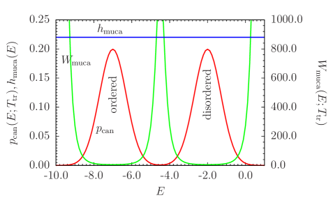
Fig. 1: Typical scenario of a first-order transition at transition temperature $T_{\text{tr}}$: Ordered and disordered phases, represented by the peaked sections of the canonical energy distribution $p_{\text{can}}(E;T_{\text{tr}})$ at low and high energies, are separated by an entropically strongly suppressed energetic region. The multicanonical weight function $W_{\text{muca}}(E;T_{\text{tr}})$ is chosen in such a way that multicanonical sampling provides a random walk in energy space, independently of (energetic) free-energy barriers. Thus, the energy distribution $h_{\text{muca}}(E)$ is ideally constant in the multicanonical ensemble.

Recalling that the simulation temperature $T$ does not possess any meaning in the multicanonical ensemble as, according to Eq. (23), the energy distribution is always constant, independently of temperature. Actually, it is convenient to set it to infinity in which case $\lim_{T\to\infty}p_{\rm can}(E;T)\sim g(E)$ and thus $\lim_{T\to\infty}W_{\rm muca}(E;T)\sim g^{-1}(E)$. Then, the acceptance probability (10) is governed by

$$w({\bf X}\to{\bf X}^{\prime})=W_{\text{muca}}(E({\bf X}^{\prime}))/W_{\text{muca}}(E({\bf X}))=g(E({\bf X}))/g(E({\bf X}^{\prime})).$$ (24)

The weight function can suitably be parametrized as

$$W_{\text{muca}}(E)\sim\exp[-S(E)/k_{\text{B}}]=\exp\{-\beta(E)[E-F(E)]\},$$ (25)

where $S(E)$ is the microcanonical entropy $S(E)=k_{\text{B}}\ln g(E)$. Since $\beta(E)=\partial S(E)/\partial E$ is the microcanonical thermal energy (with $\beta(E)=1/k_{\text{B}}T(E)$, where $T(E)$ is the microcanonical temperature), the microcanonical free-energy scale $f(E)=\beta(E)F(E)$ and $\beta(E)$ are related to each other by the differential equation

$$\frac{\partial f(E)}{\partial E}=\frac{\partial\beta(E)}{\partial E}E.$$ (26)

Since $\beta(E)$ and $f(E)$ are unknown in the beginning of the simulation, this relation must be solved recursively. This can be done in an efficient way [16, 17, 19]. If not already being discrete by the model definition, the energy spectrum must be discretized, i.e., neighboring energy bins are separated by an energetic step size $\varepsilon$. Thus, for the estimation of $\beta(E)$ and $f(E)$, the following system of difference equations needs to be solved recursively ($s(E)=S(E)/k_{\text{B}}$):

$$s^{(n-1)}(E) = \ln g^{(n-1)}(E)=-\ln W^{(n-1)}_{\text{muca}}(E)$$

$$\beta^{(n)}(E) = [s^{(n-1)}(E)-s^{(n-1)}(E-\varepsilon)]/\varepsilon$$

$$f^{(n)}(E) = f^{(n)}(E-\varepsilon)+[\beta^{(n)}(E)-\beta^{(n)}(E-\varepsilon)](E-\varepsilon)$$ (27)

$$s^{(n)}(E) = \beta^{(n)}(E)E-f^{(n)}(E)$$

$$W^{(n)}_{\text{muca}}(E) = \exp[-s^{(n)}(E)].$$

The superscript $(n)$ refers to the index of the iteration. If no better initial guess is available, one typically sets $g^{(0)}(E)=1$ in the beginning, implying $s^{(0)}(E)=W^{(0)}_{\text{muca}}(E)=0$. The zeroth iteration thus corresponds to a Metropolis run at infinite temperature, yielding the first estimate for the multicanonical weight function $W^{(1)}_{\text{muca}}(E)$, which is used to initiate the second recursion, etc. The recursion procedure based on Eq. (4.2) can be stopped after $I$ recursions, if the weight function has sufficiently converged. The number of necessary recursions and also the number of sweeps to be performed within each recursion is model dependent. Since the sampled energy space increases from recursion to recursion and the effective statistics of the histogram in each energy bin depends on the number of sweeps, it is a good idea to increase the number of sweeps successively from recursion to recursion. Since the energy histogram should be “flat” after the simulation run at a certain recursion level, an alternative way to control the length of the run is based on a flatness criterion. If, for example, minimum and maximum value of the histogram deviate from the mean histogram value by less than 20%, the run is stopped.

Finally, after the best possible estimate for the multicanonical weight function is obtained, a long multicanonical production run is performed, including all measurements of quantities of interest. From the multicanonical trajectory, the estimate of the canonical expectation value of a quantity $O$ is then obtained at any (canonical) temperature $T$ by:

$$\overline{O}_{T}=\frac{\sum_{t}O(\textbf{X}_{t})W^{-1}_{\text{muca}}(E(\textbf{X}_{t})e^{-E(\textbf{X}_{t})/k_{\text{B}}T}}{\sum_{t}W^{-1}_{\text{muca}}(E(\textbf{X}_{t})e^{-E(\textbf{X}_{t})/k_{\text{B}}T}}.$$ (28)

Since the accuracy of multicanonical sampling is independent of the canonical temperature and represents a random walk in the entire energy space, the application of reweighting procedures is lossless. This is a great advantage of the multicanonical method, compared with Metropolis Monte Carlo simulations. Virtually, a multicanonical simulation samples the system behavior at all temperatures simultaneously, or, in other words, the direct estimation of the density of states is another advantage, because multiple-histogram reweighting is not needed for this (in contrast to replica-exchange methods).

4.3 Wang-Landau method

In multicanonical simulations, the weight functions are updated after each iteration, i.e., the weight and thus the current estimate of the density of states are kept constant at a given recursion level. For this reason, the precise estimation of the multicanonical weights in combination with the recursion scheme (4.2) can be a complex and not very efficient procedure. In the method introduced by Wang and Landau [20], the density of states estimate is changed by a so-called modification factor $\alpha$ after each sweep, $g(E)\to\alpha^{(n)}g(E)$, where $\alpha^{(n)}>1$ is kept constant in the $n$th recursion, but it is reduced from iteration to iteration. A frequently used ad hoc modification factor is given by $\alpha^{(n)}=\sqrt{\alpha^{(n-1)}}=(\alpha^{(0)})^{1/2^{n}}$, $n=1,2,\ldots,I$, where often $\alpha^{(0)}=e^{1}=2.718\ldots$ is chosen. The acceptance probability and histogram flatness criteria are the same as in multicanonical sampling.

Since the dynamic modification of the density of states in the running simulation violates the detailed balance condition (7), the advantage of the high-speed scan of the energy space is paid by a systematic error. However, since the modification factor is reduced with increasing iteration level until it is very small (the iteration process is typically stopped if $\alpha<1.0+10^{-8}$), the simulation dynamics is supposed to sample the phase space according to the stationary solution of the master equation such that detailed balance is (almost) satisfied. Since it is difficult to keep this convergence under control, the optimal method is to use the Wang-Landau method for a very efficient generation of the multicanonical weights, followed by a long multicanonical production run (i.e., at exactly $\alpha=1$) to obtain the statistical data.

5 Summary

Monte Carlo computer simulations are virtually the only way to analyze the thermodynamic behavior of a system in a precise way. However, the various existing methods exhibit extreme differences in their efficiency, depending on model details and relevant questions. The original standard method, Metropolis Monte Carlo, which provides only reliable statistical information at a given (not too low) temperature has meanwhile been replaced by more sophisticated methods which are typically far more efficient (the differences in time scales can be compared with the age of the universe). However, none of the methods yields automatically accurate results, i.e., a system-specific adaptation and control is always needed. Thus, as in any good experiment, the most important part of the data analysis is statistical error estimation.

References

- [1] See, e.g., R. Kubo, Rep. Prog. Phys. 29, 255 (1966).
- [2] D. Frenkel and B. Smith, Understanding Molecular Simulation (Academic Press, San Diego, 2002).
- [3] J. Schluttig, M. Bachmann, and W. Janke, J. Comput. Chem. 29, 2603 (2008).
- [4] See, e.g., L. P. Kadanoff, Physica A 163, 1 (1990).
- [5] D. P. Landau and K. Binder, A Guide to Monte Carlo Simulations in Statistical Physics (Cambridge University Press, New York, 2009).
- [6] W. Janke, Statistical Analysis of Simulations: Data Correlations and Error Estimation, in Proceedings of the Winter School “Quantum Simulations of Complex Many-Body Systems: From Theory to Algorithms”, John von Neumann Institute for Computing, Jülich, NIC Series vol. 10, ed. by J. Grotendorst, D. Marx, and A. Muramatsu (NIC, Jülich, 2002), p. 423.
- [7] R. G. Miller, Biometrika 61, 1 (1974); B. Efron, The Jackknife, the Bootstrap, and Other Resampling Plans (SIAM, Philadelphia, 1982).
- [8] G. Favrin, A. Irbäck, and F. Sjunnesson, J. Chem. Phys. 114, 8154 (2001).
- [9] N. Metropolis, A. W. Rosenbluth, M. N. Rosenbluth, A. H. Teller, and E. Teller J. Chem. Phys. 21, 1087 (1953).
- [10] A. M. Ferrenberg and R. H. Swendsen, Phys. Rev. Lett. 63, 1195 (1989).
- [11] S. Kumar, D. Bouzida, R. H. Swendsen, P. A. Kollman, and J. M. Rosenberg, J. Comput. Chem. 13, 1011 (1992).
- [12] R. H. Swendsen and J.-S. Wang, Phys. Rev. Lett. 57, 2607 (1986).
- [13] K. Hukushima and K. Nemoto, J. Phys. Soc. Jpn. 65, 1604 (1996).
- [14] C. J. Geyer, in Computing Science and Statistics, Proceedings of the 23rd Symposium on the Interface, ed. by E. M. Keramidas (Interface Foundation, Fairfax Station, 1991), p. 156.
- [15] B. A. Berg and T. Neuhaus, Phys. Lett. B 267, 249 (1991); Phys. Rev. Lett. 68, 9 (1992).
- [16] W. Janke, Physica A 254, 164 (1998); B. A. Berg, Fields Inst. Comm. 26, 1 (2000).
- [17] W. Janke, Histograms and All That, in: Computer Simulations of Surfaces and Interfaces, NATO Science Series, II. Mathematics, Physics and Chemistry – Vol. 114, edited by B. Dünweg, D. P. Landau, and A. I. Milchev (Kluwer, Dordrecht, 2003), p. 137.
- [18] M. Bachmann, H. Arkın, and W. Janke, Phys. Rev. E 71, 031906 (2005).
- [19] T. Çelik and B. A. Berg, Phys. Rev. Lett. 69, 2292 (1992).
- [20] F. Wang and D. P. Landau, Phys. Rev. Lett. 86, 2050 (2001); Phys. Rev. E 64, 056101 (2001).