Hierarchies in Nucleation Transitions

Abstract

We discuss the hierarchy of subphase transitions in first-order-like nucleation processes for an examplified aggregation transition of heteropolymers. We perform an analysis of the microcanonical entropy, i.e., the density of states is considered as the central statistical system quantity since it connects system-specific entropic and energetic information in a natural and unique way.

url]www.smsyslab.org

1 Introduction

The noncovalent cooperative effects in structure formation processes on mesoscopic scales let linear polymers be very interesting objects for studies of the statistical mechanics and thermodynamics of nucleation processes, even on a fundamental level. Structural properties of polymers can typically be well described by means of simple, coarse-grained models of beads and sticks (or springs) representing the monomers and the covalent bonds between adjacent monomers in the chain, respectively. Contemporary, sophisticated generalized-ensemble Monte Carlo simulation techniques as well as large-scale computational resources enable the precise and systematic analysis of thermodynamic properties of all structural phases of coarse-grained polymer models by means of computer simulations. Among the most efficient simulations methods are multicanonical sampling [1, 2], replica-exchange techniques [3, 4], and the Wang-Landau method [5].

The high precision of the numerical data for quantities that are hardly accessible in analytic calculations – one of the most prominent and, as it will turn out in the following, most relevant system-specific quantities is the density (or number) of states with energy $E$, $g(E)$ – opens new perspectives for the physical interpretation and classification of cooperative processes such as phase transitions. This is particularly interesting for small systems, where conventional statistical analyses are often little systematic and a general concept seems to be missing. This is apparently reflected in conformational studies in the biosciences, where often novel terminologies are invented for basically the same classes of transitions. The introduction of a unifying scheme appears insofar difficult as finite-size effects in transitions of small systems influence the thermal fluctuations of transition indicators like order parameters. Maximum energetic fluctuations, represented by peaks in the specific heat, do not necessarily coincide with peak temperatures of fluctuations of structural quantities such as the radius of gyration [6, 7]. For extremely large systems, which are well described by the theoretical concept of the “thermodynamic limit”, this canonical approach is appealing as the fluctuation peaks scale with system size and finally collapse at the same temperature, allowing for the definition of a unique transition point. However, for many systems, in particular biomolecules, the assumption of the thermodynamic limit is nonsensical and the explicit consideration and understanding of finite-size effects is relevant.

2 Microcanonical vs. canonical temperature

The microcanonical analysis [8] allows for such an in-depth analysis of smallness effects. It is completely based on the entropy as a function of the system energy, which is related to the density of states via $S(E)=k_{\rm B}\ln\,g(E)$, where $k_{\rm B}$ is the Boltzmann constant. A major advantage of this quantity is the possibility to introduce the temperature as a derived quantity via

$$T(E)=\left[\frac{\partial S(E)}{\partial E}\right]^{-1}$$ (1)

which is commonly refered to as the “microcanonical temperature”. This terminology is misleading since $S(E)$ and thus $T(E)$ do not depend on the choice of any statistical ensemble associated to a certain thermal environment of the system. Thus, the physical meaning of $S(E)$ and $T(E)$ is not restricted to systems well-described by the microcanonical ensemble only (i.e., for systems with constant energy). The introduction of the temperature via Eq. (1) is also useful for another reason. It applies independently of the system size and it is not coupled to any equilibrium condition. To make use of theoretical concepts like the thermodynamic limit or quasiadiabatic process flow is not necessary.

The typically used heatbath concept for introducing the temperature in the context of the thermodynamic equilibrium of heatbath and system is useful for large systems when thermal fluctuations become less relevant and finite-size effects disappear. However, as it has already been known from the early days of statistical mechanics, the statistical ensembles turn over to the microcanonical ensemble in the thermodynamic limit. This is easily seen for the example of the fluctuations about the mean energy in the canonical ensemble. In this case, the canonical statistical partition function, linked to the free energy $F(T^{\rm can}_{\rm system})$, can be written as an integral over the energy space,

$$Z(T^{\rm can}_{\rm system})=\int_{E_{\rm min}}^{E_{\rm max}}dEg(E)e^{-E/k_{\rm B}T^{\rm can}_{\rm system}}=e^{F/k_{\rm B}T^{\rm can}_{\rm system}},$$ (2)

where the canonical system temperature $T^{\rm can}_{\rm system}$ corresponds in equilibrium to the heatbath temperature $T_{\rm heatbath}$ (which is an adjustable external thermal control parameter in experiments):

$$T^{\rm can}_{\rm system}\equiv T_{\rm heatbath}.$$ (3)

Therefore, in equilibrium, the mean energy at a given heatbath temperature can simply be calculated as:

$$\langle E\rangle(T_{\rm heatbath})=\frac{1}{Z(T_{\rm heatbath})}\int dE\,E\,g(E)e^{-E/k_{\rm B}T_{\rm heatbath}}.$$ (4)

The heat capacity $C_{V}(T_{\rm heatbath})=d\langle E\rangle/dT_{\rm heatbath}=(\langle E^{2}\rangle-\langle E\rangle^{2})/k_{\rm B}T_{\rm heatbath}^{2}$ must always be nonnegative because of the thermodynamic stability of matter, i.e., $\langle E\rangle$ increases monotonously with $T_{\rm heatbath}$. For this reason, the dependence of $\langle E\rangle$ on the temperature can trivially be inverted, $T^{\rm can}_{\rm system}(\langle E\rangle)$, where we have made use of the equilibrium condition (3). In complete analogy to the microcanonical definition of the temperature in Eq. (1), we introduce the canonical entropy via the relation

$$T^{\rm can}_{\rm system}(\langle E\rangle)=\left[\frac{\partial S^{\rm can}(\langle E\rangle)}{\partial\langle E\rangle}\right]_{N,V}^{-1},$$ (5)

where particle number $N$ and volume $V$ are kept constant. The canonical entropy can explicitly be expressed by the celebrated equation that links thermodynamics and statistical mechanics:

$$S^{\rm can}(\langle E\rangle)=\frac{1}{T^{\rm can}_{\rm system}(\langle E\rangle)}\left[\langle E\rangle-F(T^{\rm can}_{\rm system}(\langle E\rangle))\right].$$ (6)

Instead of considering the canonical ensemble by fixing $T_{\rm heatbath}$, $V$, and $N$ as external parameters, we have turned to the caloric representation, where $\langle E\rangle$, $V$, and $N$ are treated as independent variables. If the fluctuations of energy about the mean value $\langle E\rangle$ vanish, the canonical ensemble thus corresponds to the microcanonical ensemble. This is obvious in the thermodynamic limit, where the relative width of the canonical energy distribution, $\Delta E/\langle E\rangle=\sqrt{\langle E^{2}\rangle-\langle E\rangle^{2}}/\langle E\rangle=\sqrt{k_{\rm B}T_{\rm heatbath}^{2}C_{V}(T_{\rm heatbath})}/\langle E\rangle\propto 1/\sqrt{N}$ vanishes, $\lim_{N\to\infty}(\Delta E/\langle E\rangle)=0$, since $C_{V}$ and $\langle E\rangle$ are extensive variables as they scale with $N$. Thus, $\langle E\rangle=E$ and $T(E)=T^{\rm can}_{\rm system}(\langle E\rangle)$ in the thermodynamic limit.

3 Small systems

Microcanonical and canonical temperatures do typically not coincide, if finite-size effects matter. This is particularly apparent under conditions where cooperative changes of macrostates, such as conformational transitions of finite molecular systems, occur. In transitions with structure formation, the conformational entropies associated to volume and surface effects in the formation of compact states of the system compete with the energetic differences of particles located at the surface or in the interior of the structure. Examples for such morphologies of finite size are atomic clusters, spin clusters, the interface of demixed fluids, globular polymers or proteins, crystals, etc. Since many interesting systems such as heterogeneous biomolecules like proteins are “small” in a sense that a thermodynamic limit does not exist at all, it is useful to build up the analysis of transitions of small systems on the most general grounds. These are, as we have argued above, best prepared by the microcanonical or caloric approach.

The folding of a protein is an example for a subtle structure formation process of a finite system, where effects on nanoscopic scales (e.g., hydrogen bonds being responsible for local secondary structures such as helices and sheets) and cooperative behavior on mesoscopic scales (such as the less well-defined hydrophobic effect which primarily drives the formation of the global, tertiary structures) contribute to the stable assembly of the native fold which is connected to the biological function of the protein. Proteins are linear polypeptides, i.e., they are composed of amino acids linked by peptide bonds. There are twenty types of amino acids that have been identified in bioproteins, all of them differ in their chemical composition and thus possess substantial differences in their physical properties and chemical reactivity. The mechanism of folding depends on the sequence of amino acids, not only the content, i.e., a protein is a disordered system. It is one of the central questions, which mutations of a given amino-acid sequence can lead to a relevant change of morphology and thus the loss of functionality. The atomistic interaction types, scales, and ranges are different as well. For this reason, in compact folds, frustration effects may occur. Disorder and frustration cause glassy behavior, but how glassy is a single protein and can this be generalized?

Since details seem to be relevant for folding, it has commonly been believed that the folding of a certain protein is a highly individual process. Thus, it was a rather surprising discovery that the search for a stable fold can be a cooperative one-step process which can qualitatively and quantitatively be understood by means of the statistical analysis of a single effective, mesoscopic order parameter. The free-energy landscape turned out to be very simple (exhibiting only a single barrier between folded and unfolded conformations) for this class of “two-state folders” [9, 10]. Of course, folding pathways for other proteins can be more complex as also intermediate states can occur [11, 12]. However, this raises the question about cooperativity and the generalization of folding behavior in terms of conformational transitions similar to phase transitions in other fields of statistical mechanics. In the following, we are going to discuss a structure formation process, the aggregation of a finite system of heteropolymers, by a general microcanonical approach in order to show how the conformational transition behavior of a small system is indeed related to thermodynamic phase transitions.

4 Exemplified nucleation process: Aggregation of proteins

As an example for the occurrence of hierarchies of subphase transitions accompanying a nucleation process, we are going to discuss molecular aggregation [13, 14, 15] by means of a simple coarse-grained hydrophobic-polar heteropolymer model [16, 17]. In this so-called AB model, only hydrophobic (A) and hydrophilic (B) monomers line up in linear heteropolymer sequences. In the following, we consider the aggregation of four chains with 13 monomers [14]. All chains have the same Fibonacci sequence $AB_{2}\-AB_{2}\-ABAB_{2}\-AB$ [16]. Folding and aggregation of this heteropolymer have already been subject of former studies [13, 14].

In the model used here, bonds between adjacent monomers have fixed length unity. Nonbonded monomers of individual chains but likewise monomers of different chains interact pairwisely via Lennard-Jones-like potentials. The explicit form of the potentials depends on the types of the interacting monomers. Pairs of hydrophobic and unlike monomers attract, pairs of polar monomers repulse each other. This effectively accounts for the hydrophobic-core formation of proteins in polar solvent. Details of our aggregation model and of the implementation of the multicanonical Monte Carlo simulation method are described in Ref. [14].

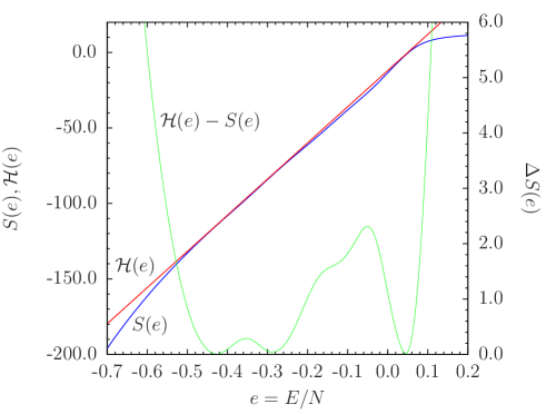
Figure 1: Microcanonical entropy $S(e)$, the Gibbs hull ${\cal H}(e)$, and the deviation $\Delta S(e)={\cal H}(e)-S(e)$ as functions of the energy per monomer.

The multicanonical computer simulations enabled us to obtain a precise estimate for the microcanonical entropy $S(E)$ of the multiple-chain system [14], as shown in Fig. 1 as a function of the energy per monomer, $e=E/N$. The entropy curve is convex in the energetic aggregation transition region as expected for a first-order-like nucleation transition of a finite system [8]. The Gibbs tangent ${\cal H}(e)$, connecting the two coexistence points where concave and convex behavior change, provides the least possible overall concave shape of $S(e)$ in this region. The difference between the Gibbs hull and the entropy curve, $\Delta S(e)={\cal H}(e)-S(e)$, is also shown in Fig. 1. Not only the entropic suppression in the transition region is clearly visible, it is also apparent that the transition possesses an internal structure.

In order to better understand the subphases, we discuss in the following the inverse derivative of the entropy, the microcanonical temperature (1), $T(e)$, which is plotted in Fig. 2. The slope of the Gibbs tangent corresponds to the Maxwell line in Fig. 2 at the aggregation temperature $T_{\rm agg}\approx 0.217$. Therefore, the intersection points of the Maxwell line and the temperature curve define the energetic phase boundaries $e_{\rm agg}$ and $e_{\rm frag}$, respectively, as both phases coexist at $T_{\rm agg}$.

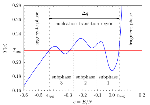
Figure 2: Microcanonical temperature $T(e)$ as a function of energy per monomer, $e=E/N$, where $N$ is the total number of all monomers in the system. The horizontal Maxwell line marks the aggregation temperature $T_{\rm agg}$, obtained by the Gibbs construction. Vertical dashed lines separate the different phases and subphases, respectively.

For energies $e<e_{\rm agg}\approx-0.43$, conformations of a single aggregate, composed of all four chains, dominate. On the other hand, conformations with $e>e_{\rm frag}\approx 0.05$ are mainly entirely fragmented, i.e., all chains can form individual conformations, almost independently of each other. The entropy is governed by the contributions of the individual translational entropies of the chains, outperforming the conformational entropies. The translational entropies are only limited by the volume which corresponds to the simulation box size. The energetic difference $\Delta q=e_{\rm frag}-e_{\rm agg}$, serving as an estimator for the latent heat, is obviously larger than zero, $\Delta q\approx 0.48$. It thus corresponds to the total energy necessary to entirely melt the aggregate into fragments at the aggregation (or melting) temperature.

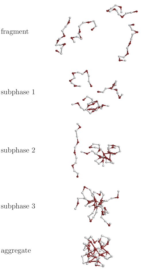
Figure 3: Representative conformations in the different structural phases.

The relation between energy and microcanonical temperature in the aggregate phase and in the fragment phase is as intuitively expected: With increasing energy, also $T(e)$ increases. However, much more interesting is the behavior of the system in the energy interval $e_{\rm agg}<e<e_{\rm frag}$, which represents the energetic nucleation transition region. Figure 2 clearly shows that in our example $T(e)$ changes the monotonic behavior three times in this regime. Representative conformations in the diffferent structural phases are shown in Fig. 3. The change of monotony of the microcanonical temperature curve is called backbending effect, because the temperature decreases while energy is increased. This rather little intuitive behavior is a consequence of the suppression of entropy in this regime ($S(E)$ is convex in the backbending region). The surface entropy per monomer vanishes in the thermodynamic limit [14].

If two chains aggregate (subphase 1 in Fig. 2), the total translational entropy of the individual chains is reduced by $k_{B}\ln\,V$, where $V$ is the volume (corresponding to the simulation box size), whereas the energy of the aggregate is much smaller than the total energy of the system with the individual chains separated. Thus, the energy associated to the interaction between different chains, i.e., the cooperative formation of inter-chain contacts between monomers of different chains, is highly relevant here. This causes the latent heat between the completely fragmented and the two-chain aggregate phase to be nonzero which signals a first-order-like transition. This procedure continues when an additional chain joins a two-chain cluster. Energetically, the system enters subphase 2. Qualitatively, the energetic and entropic reasons for the transition into this subphase are the same as explained before, since it is the same kind of nucleation process. In our example of four chains interacting with each other, there is another subphase 3 which also shows the described behavior. The energetic width of each of the subphase transitions corresponds to the respective latent heat gained by adding another chain to the already formed cluster. The subphase boundaries (vertical dashed, gray lines in Fig. 2) have been defined to be the inflection points in the raising temperature branches, thus enclosing a complete “oscillation” of the temperature as a function of energy. The energetic subphase transition points are located at $e_{\rm 12}\approx-0.11$ and $e_{\rm 23}\approx-0.26$, respectively. Therefore, the latent heat associated to these subphase transitions is in all three cases about $\Delta q_{ij}\approx 0.16$ ($i,j=1,2,3$, $i\neq j$), thus being one third of the total latent heat of the complete nucleation process. This reflects the high systematics of subphase transitions in first-order nucleation processes.

5 Summary

The most interesting result from this heteropolymer aggregation study is that first-order phase transitions such as nucleation processes can be understood as a composite of hierarchical subphase transitions, each of which exhibits features of first-order-like transitions. Since with increasing number of chains the microcanonical entropy per chain converges to the Gibbs hull in the transition region, the “amplitudes” of the backbending oscillations and the individual latent heats of the subphases become smaller and smaller [14, 15]. Thus, in the thermodynamic limit, the heteropolymer aggregation transition is a first-order nucleation process composed of an infinite number of infinitesimally “weak” first-order-like subphase transitions.

References

- [1] B. A. Berg and T. Neuhaus, Phys. Lett. B 267, 249 (1991); Phys. Rev. Lett. 68, 9 (1992).
- [2] W. Janke, Physica A 254, 164 (1998); B. A. Berg, Fields Inst. Comm. 26, 1 (2000).
- [3] K. Hukushima and K. Nemoto, J. Phys. Soc. Jpn. 65, 1604 (1996).
- [4] C. J. Geyer, in Computing Science and Statistics, Proceedings of the 23rd Symposium on the Interface, ed. by E. M. Keramidas (Interface Foundation, Fairfax Station, 1991), p. 156.
- [5] F. Wang and D. P. Landau, Phys. Rev. Lett. 86, 2050 (2001).
- [6] M. Bachmann and W. Janke, in: Rugged Free Energy Landscapes: Common Computational Approaches to Spin Glasses, Structural Glasses and Biological Macromolecules, edited by W. Janke, Lect. Notes Phys. 736 (Springer, Berlin, 2008), p. 203.
- [7] M. Bachmann and W. Janke, J. Chem. Phys. 120, 6779 (2004).
- [8] D. H. E. Gross, Microcanonical Thermodynamics (World Scientific, Singapore, 2001).
- [9] S. E. Jackson and A. R. Fersht, Biochemistry 30, 10428 (1991).
- [10] A. R. Fersht, Structure and Mechanisms in Protein Science: A Guide to Enzyme Catalysis and Protein Folding (Freeman, New York, 1999).
- [11] S. Schnabel, M. Bachmann, and W. Janke, Phys. Rev. Lett. 98, 048103 (2007).
- [12] S. Schnabel, M. Bachmann, and W. Janke, J. Chem. Phys. 126, 105102 (2007).
- [13] C. Junghans, M. Bachmann, and W. Janke, Phys. Rev. Lett. 97, 218103 (2006).
- [14] C. Junghans, M. Bachmann, and W. Janke, J. Chem. Phys. 128, 085103 (2008).
- [15] C. Junghans, M. Bachmann, and W. Janke, Europhys. Lett. 87, 40002 (2009).
- [16] F. H. Stillinger, T. Head-Gordon, and C. L. Hirshfeld, Phys. Rev. E 48, 1469 (1993); F. H. Stillinger and T. Head-Gordon, Phys. Rev. E 52, 2872 (1995).
- [17] M. Bachmann, H. Arkın, and W. Janke, Phys. Rev. E 71, 031906 (2005).