The Physical Basis for Long-lived Electronic Coherence in Photosynthetic Light Harvesting Systems

Abstract

The physical basis for observed long-lived electronic coherence in photosynthetic light-harvesting systems is identified using an analytically soluble model. Three physical features are found to be responsible for their long coherence lifetimes: i) the small energy gap between excitonic states, ii) the small ratio of the energy gap to the coupling between excitonic states, and iii) the fact that the molecular characteristics place the system in an effective low temperature regime, even at ambient conditions. Using this approach, we obtain decoherence times for a dimer model with FMO parameters of $\approx$ 160 fs at 77 K and $\approx$ 80 fs at 277 K. As such, significant oscillations are found to persist for 600 fs and 300 fs, respectively, in accord with the experiment and with previous computations. Similar good agreement is found for PC645 at room temperature, with oscillations persisting for 400 fs. The analytic expressions obtained provide direct insight into the parameter dependence of the decoherence time scales.

Electronic energy transfer is ubiquitous in nature and its dynamics and manipulation is of special interest in diverse fields of physics, chemistry, biology and engineering. Under natural conditions loss of coherence is expected to occur on ultrashort times scale due to interaction with the environment. For example, results on betaine dye molecules Hwang and Rossky (2004a) and on femtosecond dynamics and laser control of charge transport in trans-polyacetylene Franco et al. (2008) suggest that these time scales are very short, $\sim$2.5 fs and $\sim$3.7 fs, respectively. At high temperatures and for weak coupling to the environment, a classical treatment of the thermal fluctuations suggests that this time scale can be determined as $\tau_{\mathrm{G}}=\sqrt{\hbar^{2}/2\lambda k_{\mathrm{B}}T}$ where $\lambda$ is the system reorganization energy Hwang and Rossky (2004b); Gilmore and McKenzie (2008). Based on this expression, the dephasing time for photosynthetic complexes, the systems of interest in this paper, (wherein a typical value of the reorganization energy is $\lambda=130$ cm^-1), can be estimated Cheng and Fleming (2009) to be $\tau_{\mathrm{G}}=45$ fs at $T=77$ K and $\tau_{\mathrm{G}}=23$ fs and $T=294$ K.

By contrast, recent experiments in photosynthetic complexes such as the FMO complex Engel et al. (2007); Panitchayangkoon et al. (2010) and the PC645 complex Collini et al. (2010) have found that electronic coherences among different chromophores survive up to 800 fs at $77$ K Engel et al. (2007) and up 400 fs at room temperature Collini et al. (2010); Panitchayangkoon et al. (2010). This surprising observation and its possible consequences for biological processes have been discussed extensively Engel et al. (2007); Plenio and Huelga (2008); Panitchayangkoon et al. (2010); Cheng and Fleming (2009); Rebentrost et al. (2009); Ishizaki and Fleming (2009); Wu et al. (2010); Collini et al. (2010); Briggs and Eisfeld (2011); Huo and Coker (2011); Shim et al. (2011); Nalbach et al. (2011) and very elaborate models have been developed in order to understand the underlying dynamics Ishizaki and Fleming (2009); Briggs and Eisfeld (2011); Huo and Coker (2011); Shim et al. (2011); Nalbach et al. (2011). Interestingly, despite the diversity of approaches and techniques, most Cheng and Fleming (2009); Rebentrost et al. (2009); Ishizaki and Fleming (2009); Collini et al. (2010); Briggs and Eisfeld (2011); Huo and Coker (2011); Shim et al. (2011); Nalbach et al. (2011) now predict long-lived coherences on the same times scales as found experimentally Engel et al. (2007); Collini et al. (2010); Panitchayangkoon et al. (2010). This suggests that the underlying physical features are correctly contained in these approaches. However, the sheer complexity of these computations has limited one from identifying these essential physical features.

In this paper we present a simple analytic approach that provides deep insights into the long lived coherences in the evolution of FMO complexes Engel et al. (2007); Panitchayangkoon et al. (2010); Cheng and Fleming (2009); Rebentrost et al. (2009); Ishizaki and Fleming (2009); Collini et al. (2010); Briggs and Eisfeld (2011); Shim et al. (2011) and PC645 Collini et al. (2010); Huo and Coker (2011) and allows for the identification of central characteristics responsible for these long lived coherences. Our analysis identifies the small effective temperature of the system (see below), the very small, but nonzero, energy gap between exciton states, and their coupling as the basic elements behind these long lifetimes. Given these conditions, we show that the lifetimes are not “surprisingly long”. As such, the challenge now reverts to, for example, obtaining an atomistic understanding Shim et al. (2011) of the origins of these parameter values.

Consider first results for the Fenna-Matthews-Olson (FMO) complexes, in particular the FMO pigment-protein complex from Chlorobium tepidum Engel et al. (2007); Panitchayangkoon et al. (2010). This is a trimer consisting of identical, weakly interacting monomers Adolphs and Renger (2006). Each weakly interacting FMO monomer contains seven coupled bacteriochlorophyll-$a$ (BChl$a$) chromophores arranged asymmetrically, yielding seven nondegenerate, delocalized molecular excited states (excitons) Engel et al. (2007); Panitchayangkoon et al. (2010). Since the electronic coupling between the BChl$a$ 1 and BChl$a$ 2 is relatively strong in comparison with the other coupling strengths Adolphs and Renger (2006), we can approximate the dynamics of the excitation as given by a dimer composed by BChl$a$ 1 and BChl$a$ 2. This, often adopted, approximation is utilized below.

We consider the dimer (see 1) to be described by the Hamiltonian Gilmore and McKenzie (2005, 2006)

$$\begin{split}H&=\frac{\hbar}{2}\epsilon_{1}\sigma_{z,1}+\frac{\hbar}{2}\epsilon_{2}\sigma_{z,2}+\frac{\hbar}{2}\Delta\left(\sigma_{x,1}\sigma_{x,2}+\sigma_{y,1}\sigma_{y,2}\right)\\ &+\frac{\hbar}{2}\delta\mu_{1}\sigma_{z,1}R_{1}+\frac{\hbar}{2}\delta\mu_{2}\sigma_{z,2}R_{2}+B_{1}+B_{2},\end{split}$$ (1)

where $R_{i}=\sum_{\alpha}C_{\alpha,i}\left(a_{\alpha,i}+a_{\alpha,i}^{\dagger}\right)$ is the reaction field operator for molecule $i$, $B_{i}=\sum_{\alpha}\hbar\omega_{\alpha,i}a_{\alpha,i}^{\dagger}a_{\alpha,i}$ is the energy stored in the solvent cage of molecule $i$ and $\delta\mu_{j}$ is the difference between the dipole moment of the chromophore $j$ in the ground and excited states Gilmore and McKenzie (2005, 2006). The first two terms in 1 are the contributions from the individual sites and the third term is the $\Delta$ coupling between them. The subsequent terms describe the system-bath coupling. Following references 19 and 20, the Hamiltonian in 1 can be written with respect to the basis $\{|g_{1}\rangle\otimes|g_{2}\rangle,|g_{1}\rangle\otimes|e_{2}\rangle,|e_{1}\rangle\otimes|g_{2}\rangle,|e_{1}\rangle\otimes|e_{2}\rangle\}$ describing the state of the two chromophores, i.e.

$$H=\sum_{\stackrel{{\scriptstyle\alpha}}{{i=1,2}}}\hbar\omega_{\alpha,i}a_{\alpha,i}^{\dagger}a_{\alpha,i}$$ (2)

$$+\frac{\hbar}{2}\left(\begin{array}[]{cccc}-\left(\epsilon_{+}+V_{+}\right)&0&0&0\\[5.69054pt] 0&-\left(\epsilon_{-}+V_{-}\right)&2\Delta&0\\[5.69054pt] 0&2\Delta&\epsilon_{-}+V_{-}&0\\[5.69054pt] 0&0&0&\epsilon_{+}+V_{+}\end{array}\right)\,,$$

where $\epsilon_{\pm}\equiv\epsilon_{1}\pm\epsilon_{2}$, and $V_{\pm}\equiv\delta\mu_{1}R_{1}\pm\delta\mu_{2}R_{2}$.

Since under excitation by weak light only the singly excited states need to be taken into account, we can identify Gilmore and McKenzie (2006); Eckel et al. (2009) the active environment coupled 2D-subspace as $\{|e_{1}\rangle\otimes|g_{2}\rangle,|g_{1}\rangle\otimes|e_{2}\rangle\}$. In this central subspace of 2, the effective interacting biomolecular two-level system Hamiltonian reads

$$H=\left(\frac{\hbar\epsilon}{2}\sigma_{z}+\hbar\Delta\sigma_{x}\right)+\frac{\hbar}{2}\sigma_{z}V+\sum_{\stackrel{{\scriptstyle\alpha}}{{i=1,2}}}\hbar\omega_{\alpha,i}a_{\alpha,i}^{\dagger}a_{\alpha,i}\,$$ (4)

where $\epsilon\equiv\epsilon_{-}$ and $V\equiv V_{-}$. This is schematically illustrated in 1, where $\Delta$ is the associated “tunneling energy”, between the new basis states $|e_{1}\rangle\otimes|g_{2}\rangle$ and $|g_{1}\rangle\otimes|e_{2}\rangle$.

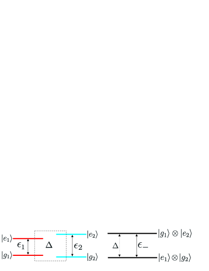
Figure 1: Left hand side: The pair of interacting chromophores. Right hand side: the effective light harvesting two-level system formed from the pair of interacting chromophores Gilmore and McKenzie (2006); Eckel et al. (2009).

Given the biophysical nanostructure composition Gilmore and McKenzie (2006), we can assume that the two bath are uncorrelated $[a_{\alpha,1},a_{\alpha,2}^{\dagger}]=0$, which implies that $\langle R_{1}(t^{\prime\prime})R_{2}(t^{\prime})\rangle=\langle R_{2}(t^{\prime\prime})R_{1}(t^{\prime})\rangle=0$. Hence, 4 can be written in the standard form of the spin-boson model Gilmore and McKenzie (2006)

$$H=\left(\frac{\hbar\epsilon}{2}\sigma_{z}+\hbar\Delta\sigma_{x}\right)+\frac{\hbar}{2}\sigma_{z}\sum_{\beta}g_{\beta}(b_{\beta}+b_{\beta}^{\dagger})+\sum_{\beta}\hbar\omega_{\beta}b_{\beta}^{\dagger}b_{\beta}\ ,$$ (5)

where the $b_{\beta}$ includes harmonic oscillators coupled to both chromophores, with couplings $g_{\beta}$.

The environment is fully characterized by the spectral density $J(\omega)=\sum_{\alpha}g_{\alpha}^{2}\delta(\omega-\omega_{\alpha})$, being a quasi-continuous function for typical condensed phase applications that determines all bath-correlations that are relevant for the system Weiss (2008); Leggett et al. (1987). For Ohmic dissipation $J(\omega)=2K\omega\,\mathrm{e}^{-\omega/\omega_{\mathrm{C}}}$, where the dimensionless parameter $K$ describes the damping strength and $\omega_{\mathrm{C}}$ is the cut-off frequency Leggett et al. (1987); Weiss (2008). An Ohmic spectral density is a useful choice for, e.g. electron transfer dynamics or biomolecular complexes May and Kühn (2001); Gilmore and McKenzie (2006). The parameter $K$ is related to the reorganization energy $\lambda$ by means of $\lambda=2K\hbar\omega_{\mathrm{C}}$ and the phonon relaxation time is given by $\tau=\pi/(2\omega_{\mathrm{C}})$ Weiss (2008); Ishizaki and Fleming (2009).

The Hamiltonian in 5 has been extensively studied in literature (cf. Chaps. 18-22 in Ref. 21 and references therein). The parameter range within which the light harvesting systems of interest lie allows for the use of the non-Markovian non-interacting blip approximation (NIBA) plus first order corrections in the interblip correlation strength, i.e. an enhanced NIBA approximation. This approximation is valid for weak system-bath coupling and for $\epsilon/2\Delta<1$, over the whole range of temperatures (see Chap. 21 in Ref. 21), and provides simple and accurate analytic expressions for relaxation and decoherence rates.

In the case of FMO, the energy gap $\epsilon$ is $(315-240)$ cm^-1 = 75 cm^-1 while the coupling energy $\Delta$ corresponds to 87.7 cm^-1 (see Ishizaki and Fleming (2009); Nalbach et al. (2011) and references therein). In accord with references 11 and 16, the reorganization energy in this case is $\lambda\approx 35$ cm^-1 and the phonon relaxation time is $\tau=50$ fs. Hence, for this case we get $K=\lambda/(2\hbar\omega_{\mathrm{C}})=\lambda\tau/(\hbar\pi)=0.105$. Additionally, at $T=77$ K, $2\Delta/k_{\mathrm{B}}T\approx 3.28$ while at $T=277$ K, $2\Delta/k_{\mathrm{B}}T\approx 0.911$. 1 summarizes the parameters of the present analysis, where we have used the same $\omega_{\mathrm{C}}$ value at both temperatures. Clearly these parameters place the system within the domain of accuracy of the enhanced NIBA approach. We emphasize that this selection of parameters is widely used in the literature Ishizaki and Fleming (2009); Nalbach et al. (2011), and it is not chosen to fit our model to the experimental results.

$\epsilon/2\Delta$	$K$	$2\Delta/\omega_{\mathrm{C}}$	$2\Delta/k_{\mathrm{B}}T$
0.428	0.105	1.052	3.28
0.428	0.105	1.052	0.911

Table 1: Parameters used for dimer formed of BChl$a$ 1 and BChl$a$ 2 at $T=77$ K (first row) and $T=277$ K (second row).

The high temperature limit in this approach is given by temperatures well in excess of $T_{\mathrm{b}}=\hbar(\Delta_{\mathrm{eff}}^{2}+\epsilon^{2})^{1/2}/k_{\mathrm{B}}$, where

$$\Delta_{\mathrm{eff}}=[\Gamma(1-2K)\cos(\pi K)]^{1/2(1-K)}(\tilde{\Delta}/\omega_{\mathrm{c}})^{K/(1-K)}\tilde{\Delta},$$

where in our case $\tilde{\Delta}=2\Delta$.

For the set of parameters listed in 1, we find $T_{\mathrm{b}}\approx 288$ K. Hence the FMO experiments, at 77 K and 277 K, are in the low temperature regime, $T<T_{\mathrm{b}}$. In this regime, the Rabi frequency $\Omega$, the relaxation rate $\gamma_{\mathrm{r}}$ and the decoherence rate $\gamma$ are given by Weiss (2008)

$$\Omega^{2} =\Delta_{\mathrm{eff}}^{2}[1-2\Re u(\mathrm{i}\Delta_{\mathrm{b}})]+\epsilon^{2}$$ (6)

$$\gamma_{\mathrm{r}} =\frac{\pi}{2}\frac{\Delta_{\mathrm{eff}}^{2}}{\Delta_{\mathrm{b}}^{2}}S(\Delta_{\mathrm{b}})$$ (7)

$$\gamma =\frac{\gamma_{\mathrm{r}}}{2}+\frac{\pi}{2}K\frac{\epsilon^{2}}{\Delta_{\mathrm{b}}^{2}}S(0),$$ (8)

respectively, where $\Delta_{\mathrm{b}}=\sqrt{\Delta_{\mathrm{eff}}^{2}+\epsilon^{2}}$ and $u(z)=\frac{1}{2}\int_{0}^{\infty}\mathrm{d}\omega\frac{J(\omega)}{\omega^{2}+z^{2}}(\coth(\hbar\omega/2k_{\mathrm{B}}T)-1)$ while $S(\omega)=J(\omega)\coth(\hbar\omega/2k_{\mathrm{B}}T)$ is the noise power. Non-Markovian corrections are already included in 6 and 8. For the particular case of Ohmic dissipation adopted here Weiss (2008),

$$\begin{split}\Omega^{2}&=\Delta_{\mathrm{b}}^{2}\\ &+2K\Delta_{\mathrm{eff}}^{2}\left[\Re\psi(\mathrm{i}\hbar\Delta_{\mathrm{b}}/2\pi k_{\mathrm{B}}T)-\ln(\hbar\Delta_{\mathrm{b}}/2\pi k_{\mathrm{B}}T)\right]\end{split}$$ (9)

$$\gamma_{\mathrm{r}} =\pi K\coth(\hbar\Delta_{\mathrm{b}}/2k_{\mathrm{B}}T)\Delta_{\mathrm{eff}}^{2}/\Delta_{\mathrm{b}},$$ (10)

$$\gamma =\gamma_{\mathrm{r}}/2+2\pi K(\epsilon^{2}/\Delta_{\mathrm{b}}^{2})k_{\mathrm{B}}T/\hbar,$$ (11)

where $\psi(z)$ is the digamma function. 10 - 11 provide simple analytic expressions for the desired rates.

With this set of expressions, and the parameters given in 1, we find $2\pi\Omega^{-1}=163$ fs, $\gamma_{\mathrm{r}}^{-1}=90$ fs, $\gamma^{-1}=153$ fs at $T=77$ K, while $2\pi\Omega^{-1}=151$ fs, $\gamma_{\mathrm{r}}^{-1}=45$ fs, $\gamma^{-1}=69$ fs at $T=277$ K. Despite the simplicity of the model, the resultant dynamics [given analytically, for general spectral densities, in Eqs. (21.79), (21.170) and (21.173) of Ref. 21] is depicted in 2 and describes the survival of coherences on the correct time scale and in good agreement with recent resultsIshizaki and Fleming (2009); Shim et al. (2011); Nalbach et al. (2011). In 2, only the decay of the excitations is absent, since coupling to other chromophores Ishizaki and Fleming (2009); Shim et al. (2011); Nalbach et al. (2011) is here neglected. The global decay in 2 is a result of two processes: one associated with the $\gamma_{\mathrm{r}}$- relaxation of the dynamics, and a second one related to the loss of coherence due to the presence of the thermal bath, associated with $\gamma$.

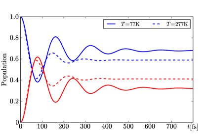
Figure 2: Time evolution of the population of the electronic manifolds $|e_{1}\rangle\otimes|g_{2}\rangle\langle g_{2}|\otimes\langle e_{1}|$ (blue curves) and $|g_{1}\rangle\otimes|e_{2}\rangle\langle e_{2}|\otimes\langle g_{1}|$ (red curves) for the FMO dimer formed of BChl$a$ 1 and BChl$a$ 2 using the parameters displayed in 1. Continuous curves depict the evolution at $T=77$ K whereas dashed curves are at $T=277$ K. We assume that at $t=0$, the full excitation is localized in $|e_{1}\rangle\otimes|g_{2}\rangle\langle g_{2}|\otimes\langle e_{1}|$.

To examine the parameter dependence, 3 shows the relaxation rate $\gamma_{\mathrm{r}}$ and the decoherence rate $\gamma$ as a function of the energy splitting, $\epsilon$, for fixed $\Delta$, using the parameters displayed in 1. Clearly in this “low temperature” regime, i.e., $T<T_{b}$, the larger the ratio $\epsilon/2\Delta$ the shorter the dephasing time and concomitantly the longer the relaxation time. These time scales are also compared in 3 with the ones predicted by $\gamma_{\phi}=2\pi(k_{\mathrm{B}}T/\hbar)\lambda/\hbar\omega_{\mathrm{C}}$ used in references 4; 10; 7 and with $\gamma_{\mathrm{G}}=1/\tau_{\mathrm{G}}$ discussed earlier, both of which are clearly far too short.

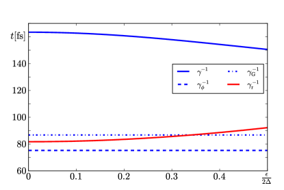
Figure 3: Relaxation time $\gamma_{\mathrm{r}}^{-1}$ (red line) and decoherence time $\gamma^{-1}$ (continuous blue line) as functions of $\epsilon/2\Delta$, for fixed $\Delta=35$ cm^-1 and at $T=77$ K. The dashed blue line, $\gamma_{\phi}=2\pi(k_{\mathrm{B}}T/\hbar)\lambda/\hbar\omega_{\mathrm{C}}$, denotes the dephasing rate used in references 4; 10; 7 and the dotdashed blue line denotes the decoherence time $\tau_{\mathrm{G}}=\sqrt{\hbar^{2}/2\lambda k_{\mathrm{B}}T}$ used in references 3; 4; 5. Fixed parameters as in 1.

As a second example we consider results on marine algae Cheng and Fleming (2009), in particular the results for PC645, which has been studied experimentally Collini et al. (2010), and numerically in great detail Huo and Coker (2011). PC645 contains eight bilin molecules covalently bound to the protein scaffold. A dihydrobiliverdin (DBV) dimer is located at the center of the complex and two mesobiliverdin (MBV) molecules located near the protein periphery give rise to the upper half of the complex absorption spectrum. Excitation of this dimer initiates the light harvesting process Collini et al. (2010). The electronic coupling between the closely spaced DBVc and DBVd molecules is $\sim$320 cm^-1 and this relatively strong coupling results in delocalization of the excitation, yielding the dimer electronic excited states labelled DBV$+$ and DBV$-$. Excitation energy absorbed by the dimer flows to the MBV molecules which are each 23 Å from the closest DBV, and ultimately to four phycocyanobilins (PCB) that absorb in the lower-energy half of the absorption spectrum Collini et al. (2010).

The exciton states related to DBVc and DBVd are mainly composed of DBV$-$ and DBV$+$ that are antisymmetric and symmetric linear combinations of the DBV sites, though they also contain small contributions from the other bilin sites Huo and Coker (2011). This allows us to concentrate only on a dimer, as in the previous example, here formed of DBVc and DBVd. In this case, a Debye-Ohmic spectral density, $J(\omega)=2\lambda\omega\tau/(1+\omega^{2}\tau^{2})$, is more appropriate Huo and Coker (2011).

For the chromophores DVBc and DVBd the energy gap is $(17116-17034)$ cm^-1 = 82 cm^-1 with the coupling energy corresponding to 319.4 cm^-1 Collini et al. (2010); Huo and Coker (2011). In accord with Ref. 14, the reorganization energy $\lambda$ in this case is $\sim$130 cm^-1, with the shorter of two relaxation times being $\tau=50$ fs. Additionally, at $T=294$ K, the temperature at which the experiment was performed, $2\Delta/k_{\mathrm{B}}T=3.1262$. For this set of parameters, we have $T_{\mathrm{b}}\sim 926$ K, a high temperature that is consistent with the high frequencies involved in the present case Galve et al. (2010). Hence the PC645 experiment, at room temperature, is also in the effective low temperature $T<T_{\mathrm{b}}$ domain. For the case of the Debye-Ohmic spectral density we have (via a relatively simple numerical computation) that $2\pi\Omega^{-1}=49$ fs, $\gamma_{\mathrm{r}}^{-1}=76$ fs, $\gamma^{-1}=88$ fs with the associated evolution shown in 4. These results are in very good qualitative agreement with both the long lived experimental coherence time scales and with the recent intricate solution to the master equations Huo and Coker (2011).

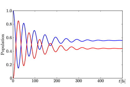
Figure 4: Time evolution of the population of the electronic manifolds $|e_{1}\rangle\otimes|g_{2}\rangle\langle g_{2}|\otimes\langle e_{1}|$ (blue curve) and $|g_{1}\rangle\otimes|e_{2}\rangle\langle e_{2}|\otimes\langle g_{1}|$ (red curve) for the PC645 DVB-dimer.

Considering that the long time scales emerge naturally here from the system parameters, why were far shorter decoherence time scales originally expected for these systems? To see this, note that in molecular systems, dynamics is often studied between different electronic eigenstates of the system, separated by greater than $\sim 10^{4}$ cm^-1, with no coupling between them. In such cases, the dephasing time from 10 and 11 would be extremely short. By contrast, in the case of photosynthetic complexes, energy transfer occurs between exciton states that are close in energy and additionally are coupled. This generates a small value for the ratio $\epsilon/\Delta$ which in turn is responsible for longer dephasing times (see 3). Additionally, expression such as $\tau_{\mathrm{G}}$, which are often used to estimate rates, are only valid at high temperature, $k_{\mathrm{B}}T\gg\hbar\omega_{\mathrm{C}}$, and at short times, $t<\omega_{\mathrm{C}}^{-1}$. Under conditions when the expression for $\tau_{\mathrm{G}}$ is valid, the bath modes can be treated classically Thoss et al. (2001), as in references 1 and 2. When one is not in the appropriate regime, the classical evolution of the bath underestimates quantum coherence effects Thoss et al. (2001) because at low temperatures quantum fluctuations overcome thermal fluctuations Hwang and Rossky (2004b). Hence, estimates based on $\tau_{G}$ are unreliable. Similarly, $\gamma_{\phi}=2\pi(k_{\mathrm{B}}T/\hbar)\lambda/\hbar\omega_{\mathrm{C}}$ estimates also provide an inadequate representation of the true physics and associated dependence on system and bath parameters, and result in decoherence times that are severely underestimated and misleading.

In summary, a proper spin-boson treatment of electronic energy transfer in model photosynthetic light harvesting systems has been shown to give analytic results with long coherence lifetimes that are in very good agreement with experiment and with other, far far more complex, computations. The analytic form allows an analysis of the parameter dependence of the decoherence times, and shows that the observed long lifetimes arise naturally in the effective low temperature regime and for appropriate ratios of the energy splitting to the coupling strength and are, in this sense, not surprisingly long. Further, the model has predictive power, allowing one to identify other parameter ranges over which longlived coherences will exist.

A more detailed analysis will involved extending this model to the 7 or 8-site system and to second order correction in the interblip approximation; work in this direction is in progress. Finally, in addition to examining other light harvesting systems, the possible application of this approach to other systems displaying long-lived coherences, such as superpositions of two excitons in quantum dots Habenicht et al. (2007) is of interest.