Molecular outflows and hot molecular cores in G24.78+0.08 at sub-arcsecond angular resolution

Abstract

Context. This study is part of a large project to study the physics of accretion and molecular outflows towards a selected sample of high-mass star-forming regions that show evidence of infall and rotation from previous studies.

Aims. We wish to make a thorough study at high-angular resolution of the structure and kinematics of the HMCs and corresponding molecular outflows in the high-mass star-forming region G24.78+0.08.

Methods. We carried out SMA and IRAM PdBI observations at 1.3 and 1.4 mm, respectively, of dust and of typical high-density and molecular outflow tracers with resolutions of $<1"$. Complementary IRAM 30-m ¹²CO and ¹³CO observations were carried out to recover the short spacing information of the molecular outflows.

Results. The millimeter continuum emission towards cores G24 A1 and A2 has been resolved into 3 and 2 cores, respectively, and named A1, A1b, A1c, A2, and A2b. All these cores are aligned in a southeast-northwest direction coincident with that of the molecular outflows detected in the region, which suggests a preferential direction for star formation in this region. The masses of the cores range from 7 to 22 $M_{\odot}$, and the rotational temperatures from 128 to 180 K. The high-density tracers have revealed the existence of 2 velocity components towards A1, one of them peaks close to the position of the millimeter continuum peak and of the HC Hii region, and is associated with the velocity gradient seen in CH₃CN towards this core, while the other one peaks southwest of core A1 and is not associated with any millimeter continuum emission peak. The position-velocity plots along outflow A and the ¹³CO (2–1) averaged blueshifted and redshifted emission indicate that this outflow is driven by core A2. Core A1 apparently is not driving any outflow. The knotty appearance of the highly collimated outflow C and the ¹²CO position-velocity plot suggest an episodic outflow, where the knots are made of swept-up ambient gas.

1 Introduction

Molecular outflows, infall and rotation are ubiquitous phenomena during the earliest stages of the formation of stars of all masses and luminosities. During the last few years, much effort has been devoted to studying and describing the physical properties of embedded massive protostars and their molecular outflows (e.g., Shepherd & Churchwell 1996a,b; Zhang et al. zhang01 (2001); Beuther et al. beuther02 (2002); López-Sepulcre lopez09 (2009)). The presence of rotating structures around massive young stars has also been asserted thanks to the detection of velocity gradients perpendicular to the axis of the molecular outflows in the cores (see Cesaroni cesa07 (2007) and reference therein). These studies have revealed two different kinds of structures surrounding B- and O-type stars. On the one hand, B-type stars are surrounded by centrifugally supported disks, as seen in the prototypical B-type protostar IRAS 20126+4104 (Cesaroni et al. cesa05 (2005); Keto & Zhang keto10 (2010)). On the other hand, despite the fact that theory predicts the existence of both large rotating structures (e.g. Peters et al. peters10 (2010)) and accretion disks (e.g. Krumholz et al. krumholz09 (2009)) around massive O-type stars, such disks have been elusive to date. One finds, instead, huge ($\sim$0.1 pc), massive (a few 100 $M_{\odot}$) rotating toroids, which are non Keplerian and very likely non-equilibrium structures (Beltrán et al. beltran11 (2011)). Finally, infall onto young O-type stars has been measured through high-angular resolution observations of lines showing redshifted self-absorption or absorption against a background bright continuum source (Keto et al. keto87 (1987); Zhang et al. zhang98 (1998); Beltrán et al. beltran06 (2006)), or by measuring the velocity field of the ionized gas surrounding a newly formed massive star (see Keto keto02 (2002)).

Table 1: Parameters of the maps

			Synthesized beama
		Frequency	$HPBW$	P.A.	Spectral resolution	rms noiseb
Observation	Telescopea	(GHz)	(arcsec)	(deg)	(km s-1)	(mJy beam-1)
continuum	SMA	225.31	$0.95\times 0.75^{\rm c}$	61c	–	3.0c
continuum	PdBI	214.30	$0.89\times 0.29$	10	–	3.2
13CH3CN (12K–11K)	PdBI	214.374d	$0.89\times 0.29^{\rm e}$	10	0.25	15
C18O (2–1)	SMA	219.560	$0.83\times 0.64^{\rm e}$	55	0.6	35
HNCO (100,10–90,9)	SMA	219.798	$0.72\times 0.51$	46	0.6	45
H213CO (31,2–21,1)	SMA	219.909	$0.72\times 0.51$	46	0.6	45
SO (65–54)	SMA	219.949	$0.83\times 0.64^{\rm e}$	55	0.6	40
CH3OH (80,8–71,6)	SMA	220.079	$0.66\times 0.48$	48	0.6	45
HCOOCH3 (172,15–164,2)	SMA	220.167	$0.71\times 0.50$	45	0.6	45
CH2CO (11,11–101,10)	SMA	220.178	$0.71\times 0.50$	45	0.6	45
HCOOCH3 (174,13–164,12)	SMA	220.190	$0.71\times 0.50$	45	0.6	45
13CO (2–1)	SMA	220.399	$0.83\times 0.64^{\rm e}$	55	1.0	35
13CO (2–1)	SMA+IRAM 30-m	220.399	$3.57\times 2.02$	71	1.0	116
CH${{}_{3}}^{13}$CN (12K–11K)	SMA	220.638d	$0.67\times 0.47$	47	0.6	45
C2H5CN (252,24–242,23)	SMA	220.661	$0.67\times 0.48$	47	0.6	45
CH3CN (12K–11K)	SMA	220.747d	$0.71\times 0.50$	46	0.6	40
CH3CN $v_{8}=1$ ( $K,l$=6,$+1$)	SMA	221.312	$0.66\times 0.47$	46	0.6	40
CH3CN $v_{8}=1$ ($K,l$=3,$-1$)	SMA	221.338	$0.66\times 0.47$	46	0.6	40
CH3OH (81,8–70,7)E	SMA	229.759	$0.65\times 0.47$	48	0.6	50
CH3OH (195,14–204,17)A$-$	SMA	229.939	$0.65\times 0.47$	47	0.6	45
CH3OH (32,2–41,4)E	SMA	230.027	$0.65\times 0.47$	48	0.6	45
12CO (2–1)	SMA	230.538	$0.86\times 0.68^{\rm e}$	54	1.5	40
12CO (2–1)	SMA+IRAM 30-m	230.538	$3.37\times 1.96$	70	1.0	116
OCS (19–18)	SMA	231.061	$0.69\times 0.50$	46	0.6	50
13CS (5–4)	SMA	231.221	$0.70\times 0.49$	46	0.6	50

^a The synthesized CLEANed beams for maps with the ROBUST parameter of Briggs (briggs95 (1995)) set equal to 0.
^b For the molecular line observations the 1$\sigma$ noise is per channel.
^c The synthesized beam for the SMA VEX configuration map is $0\aas@@fstack{\prime\prime}55\times 0\aas@@fstack{\prime\prime}40$ at P.A.=52$\degr$, and the rms noise is 3.2 mJy beam^-1.
^d The frequency is that of the $K$=0 component.
^e The synthesized CLEANed beams for maps using natural weighting.

G24.78+0.08 (hereafter G24) is one of the most studied massive star-forming regions. The simultaneous presence of the three elements fundamental for star formation (outflow, infall, and rotation) has been reported in one of the massive objects embedded in this clump. This region, which is located at a distance of 7.7 kpc, has been studied in great detail by our group (Codella et al. codella97 (1997); Furuya et al. furuya02 (2002); Cesaroni et al. cesa03 (2003); Beltrán et al. beltran04 (2004), Beltrán et al. beltran05 (2005), Beltrán et al. beltran06 (2006), Beltrán et al. beltran07 (2007); Moscadelli et al. mosca07 (2007); Vig et al. vig08 (2008)). G24 contains a cluster of Young Stellar Objects (YSOs), three of which have rotating toroids associated with them (Beltrán et al. beltran04 (2004)). These rotating toroids seem to be associated with two compact molecular outflows, first mapped in CO by Furuya et al. (furuya02 (2002)). In one of these rotating cores, G24 A1, the presence of an early-type star is witnessed by an embedded hypercompact (HC) Hii region, first detected at 1.3 cm by Codella et al. (codella97 (1997)) and later studied at very high-angular resolution at 1.3 and 0.7 cm by Beltrán et al. (beltran07 (2007)). The properties of the ionized gas have also been studied through continuum emission and recombination lines by Galván-Madrid et al. (galvan08 (2008)) and Longmore et al. (longmore09 (2009)). This HC Hii region, which has a diameter of $\la$$0\aas@@fstack{\prime\prime}2$ ($\la$1,500 AU), is located at the geometrical center of the toroid. The free-free continuum spectrum resembles that of a classical (Strömgren) Hii region around a zero-age main sequence star of spectral type O9.5, corresponding to a mass of $\sim 20\leavevmode\nobreak\ M_{\odot}$. Beltrán et al. (beltran06 (2006)) mapped the core G24 A1 in NH₃ and detected redshifted absorption, indicating that the toroid is undergoing infall towards the HC Hii region.

We have carried out new 1.3 mm interferometric observations of this region at sub-arcsecond resolution with the Submillimeter Array (SMA) (Ho et al. ho04 (2004)) of several outflow and high-density tracers. The goals of this study were to better characterize the structure and kinematics of the Hot Molecular Cores (HMCs) and molecular outflows in this region, and in particular, to identify the powering source of the outflow observed towards G24 A1. In order to be sensitive to extended structures filtered out by the interferometer, we have also mapped the region over $2^{\prime}$ with the IRAM 30-m telescope. In addition, we used the enhanced capabilities of the IRAM Plateau de Bure (PdBI) to observe this region in ¹³CH₃CN (12–11) at very high-angular resolution to investigate whether the massive toroids were hiding true (Keplerian) circumstellar disks in their interiors. Unfortunately, the angular resolution of the observations has not been enough to detect circumstellar disks embedded in the massive toroids, but it has allowed us to study the velocity structure of the cores with unprecedented resolution. The observational details are given in Sect. 2, while the results are illustrated in Sect. 3 and analyzed and discussed in Sect. 4. Finally, the conclusions are drawn in Sect. 5.

Figure 1: (Left panel) SMA map of the 1.3 mm continuum emission obtained combining both compact and very extended configurations. Contour levels are 3, 6, 9, 12, 15, 35, and 60 times $\sigma$, where 1$\sigma$ is 3 mJy beam^-1. The crosses mark the positions of the sources identified by Furuya et al. (furuya02 (2002)) and Beltrán et al. (beltran04 (2004)). The triangle marks the position of the HC Hii region in G24 A1 (Beltrán et al. beltran07 (2007)). The SMA synthesized beam is shown in the lower left corner. (Right panel) Very extended configuration only SMA map at 1.3 mm (contours) overlaid on the PdBI map at 1.4 mm (grayscale) towards G24 A1, A2 and D. Contour and grayscale levels are 3, 6, 9, 12, 15, and 20 times $\sigma$, where 1$\sigma$ is 3.2 mJy beam^-1. The SMA synthesized beam is shown in the lower left corner and the PdBI one in the lower right corner.

2 Observations

2.1 Submillimeter Array

G24 was observed with the SMA using two different array configurations. Compact-array observations were taken on July 17, 2007, and covered baselines with lengths between 7 and 100 k$\lambda$ (sampling spatial structures in the range of $29\aas@@fstack{\prime\prime}5$ to $2\aas@@fstack{\prime\prime}1$). Very Extended (VEX) configuration data were made on August 2, 2008, with baseline lengths from 23 to 391 k$\lambda$ ($9\aas@@fstack{\prime\prime}0$ to $0\aas@@fstack{\prime\prime}5$). The SMA had two spectral sidebands - both 2 GHz wide - separated by 10 GHz. For both observations, the two sidebands covered the frequency ranges of 219.3–221.3 and 229.3–231.3 GHz with a uniform spectral resolution of $\sim$0.5 km s^-1.

The phase reference center of the observations was set to the position $\alpha$(J2000)=18^h 36^m $12\aas@@fstack{s}565$, $\delta$(J2000)=$-$07^′′ 12^′ $10\aas@@fstack{\prime\prime}90$. Absolute flux calibration was derived from observations of Callisto. The bandpass of the receiver was calibrated by observations of the quasar 3C454.3. Amplitude and phase calibrations were achieved by monitoring 1733–130. The flux densities estimated for 1733$-$130 are 1.71 and 2.29 Jy for the compact and the VEX configuration, respectively. We estimate the flux-scale uncertainty to be better than 15%. The visibilities were calibrated with the IDL superset MIR. Further imaging and analysis was done with MIRIAD (Sault et al. sault95 (1995)) and GILDAS. The continuum was constructed in the (u,v)-domain from the line-free channels. Continuum and channel maps were created combining the data of both compact and VEX configurations with the ROBUST parameter of Briggs (briggs95 (1995)) set equal to 0, except for the ¹²CO, ¹³CO, C¹⁸O, and SO channel maps that were created using natural weighting. Details of the synthesized CLEANed beam, spectral resolution, and rms noise of the maps obtained in a number of lines are given in Table 1.

Table 2: Parameters of the cores

	Position peaka				Source Diametera,b
	$\alpha({\rm J2000})$	$\delta({\rm J2000})$	$I^{\rm peak}_{\nu}$	$S_{\nu}$	$\theta_{s}$	$\theta_{s}$	$T_{\rm rot}$ c	$M_{\rm gas}$ d
Core	h m s	$\degr$ $\arcmin$ $\arcsec$	(mJy/beam)	(mJy)	(arcsec)	(AU)	(K)	($M_{\odot}$)
			VEX
G24 A1	18 36 12.552	$-$07 12 10.80	86.1	187	0.47	3620	148	16e
G24 A1b	18 36 12.592	$-$07 12 11.00	38.8	57	0.31	2390	180	7
G24 A1c	18 36 12.606	$-$07 12 12.00	31.2	64	0.65	5000	146	10
G24 A2	18 36 12.464	$-$07 12 09.80	38.9	116	0.69	5315	128	22
G24 A2b	18 36 12.404	$-$07 12 08.50	24.7	39	0.49	3770	30–60	16–36
G24 C	18 36 13.096	$-$07 12 07.10	41.6	65	0.38	2925	30–60	27–60
G24 D	18 36 12.128	$-$07 12 05.80	13.6	14	0.37	2850	30–60	6–13
			VEX+compact
G24 A1+A1b+A1c			196	865			148	125f
G24 A2+A2b			107	450			128	84
G24 C			64	140			30–60	27–59
G24 D			16	14.5			30–60	7–15

^a The positions and diameters have been estimated from the very extended configuration SMA map.
^b Deconvolved average diameter of the 50% contour level.
^c From the rotational diagram method (see Sect. 4.1). For those cores for which an estimate of $T_{\rm rot}$ is not possible with this method, a range of temperatures is given.
^d Mass estimated using a dust temperature equal to $T_{\rm rot}$ and a dust opacity of 0.8 cm² g^-1 at 1.3 mm (see Sect. 4.1).
^e The dust continuum emission associated with core A1 and used to estimate the mass is 102 mJy (see Sect. 3.1).
^f The dust continuum emission associated with cores A1+A1b+A1c and used to estimate the mass is 780 mJy (see Sect. 3.1).

2.2 IRAM Plateau de Bure Interferometer

PdBI observations at 214.3 GHz in the B configuration were carried out on March 9 and 11, 2007. The correlator was set up to observe the ¹³CH₃CN (12–11) line emission at 216 GHz with both polarizations. The units of the correlator were placed in such a way that a frequency range free of lines could be used to measure the continuum flux. A unit of 80 MHz of bandwidth was set to cover the emission of ¹³CH₃CN (12–11) $K=$0 to 4, with a spectral resolution of 0.156 MHz or 0.22 km s^-1. A second unit of 320 MHz of bandwidth was set to cover the emission of ¹³CH₃CN (12–11) $K=$0 to 7, with a spectral resolution of 2.5 MHz or $\sim$3.5 km s^-1. The two remaining units of 320 MHz of bandwidth were placed to cover the rest of the band.

The phase center used was $\alpha$(J2000)=18^h 36^m $12\aas@@fstack{s}661$, $\delta$(J2000)=$-$07^′′ 12^′ $10\aas@@fstack{\prime\prime}15$. The bandpass of the receivers was calibrated by observations of the quasar 3C273. Amplitude and phase calibrations were achieved by monitoring 1741$-$038, whose flux densities were determined relative to MWC349 or 1749+096. The flux densities estimated for 1741$-$038 are 1.18 and 1.12 Jy for March 9 and 11, respectively. The uncertainty in the amplitude calibration is estimated to be $\sim$20%. The data were calibrated and analyzed with the GILDAS software package. The continuum maps were created from the line free channels. We subtracted the continuum from the line emission directly in the (u,v)-domain. Continuum and channel maps were created using natural weighting. Details of the synthesized CLEANed beam, spectral resolution, and rms noise of maps are given in Table 1.

2.3 IRAM 30-m telescope

Supplementary short-spacing information to complement the interferometric data was obtained with the IRAM 30-m telescope. The observations were carried out on November 11th, 2006 with the HERA receiver using the On-The-Fly mode. The receiver was tuned to 230.538 GHz for ¹²CO (2–1) (HERA1) and 220.399 GHz for ¹³CO (2–1) (HERA2). Both lines were observed simultaneously and covered with the VESPA autocorrelator with 0.1 km s^-1 spectral resolution, corresponding to a channel spacing of $\sim$0.07 MHz. The maps sizes were $2\arcmin\times 2\arcmin$ and were centered at $\alpha$(J2000)=18^h36^m12$\aas@@fstack{s}$6 and $\delta$(J2000)=–07°12′10$\aas@@fstack{\prime\prime}$9. The sampling interval was 2^′′ and the region was alternatively scanned in the north-south direction and the east-west direction in order to reduce effects caused by the scanning process.

The spectra were reduced using CLASS of the GILDAS software package and channel maps with 1 km s^-1 resolution were created. The ¹²CO data have a beam size of $10\aas@@fstack{\prime\prime}4$ and the ¹³CO of $10\aas@@fstack{\prime\prime}9$. The IRAM 30-m data sets were combined with the SMA data sets using the UVMODEL task of the MIRIAD package. The synthesized beam of the combined SMA+IRAM 30-m data is $3\aas@@fstack{\prime\prime}37\times 1\aas@@fstack{\prime\prime}96$ at P.A.=70$\degr$ for ¹²CO and $3\aas@@fstack{\prime\prime}57\times 2\aas@@fstack{\prime\prime}02$ at P.A.=71$\degr$ for ¹³CO

3 Results

3.1 Continuum emission

Figure 1 shows the SMA map of the 1.3 mm continuum emission towards G24. The inset shows the map obtained only from the very extended configuration at 1.3 mm towards G24 A1, A2, and D overlaid on the PdBI continuum map at 1.4 mm. The positions, fluxes, and deconvolved sizes of the cores measured as the average diameter of the 50% contour from the SMA map are given in Table 2.

As seen in Fig. 1, all but core B have been detected at 1.3 mm. The emission towards cores A1 and A2 has been resolved into additional cores with the higher angular resolution provided by the very extended configuration observations (Fig. 1). Core A1 has been resolved into 3 cores named A1, A1b, and A1c, whereas core A2 has been resolved into two named A2 and A2b. The differences between the position and geometry of cores A1c and A2b in the SMA VEX configuration map and the PdBI one are probably due to the slightly extended structure of the sources and the different (u,v)-coverage of the observations. The cores are aligned in a southeast-northwest direction coincident with that of the molecular outflow associated with cores A1 and/or A2 (see Figs. 8 and 9). The core associated with the HC Hii region is A1. To derive a rough estimate of the free-free contribution of the embedded HC Hii region at millimeter wavelengths, we extrapolated the optically thin free-free 7 mm continuum emission ($S_{\nu}\propto\nu^{-0.1}$) measured by Beltrán et al. (beltran07 (2007)). The integrated flux density at 7 mm is 101 mJy, and the expected free-free emission at 1.3 mm is $\sim$85 mJy. Therefore, the dust continuum emission associated with A1 is 102 mJy (see table 2). Note that the continuum peak intensity of core A1 is $\sim$86 mJy/beam, which is very similar to the expected free-free emission. This means that there is almost no dust emission within the HC Hii region.

Figure 2: Upper and lower sideband SMA spectra obtained by integrating the emission inside the 3$\sigma$ contour level area towards G24 A1+A2 (two upper panels) and G24 C (two lower panels). The molecular lines are marked. The different $K$-components are marked with dashed lines in the upper (lower) part of each spectrum in the case of CH₃CN (CH${{}_{3}}^{13}$CN). The $K,l$ quantum numbers of the vibrationally excited ($v_{8}=1$) CH₃CN transitions are indicated above the spectrum. Only the analyzed lines are labeled.

Figure 3: ¹³CH₃CN (12–11) spectrum obtained with the PdBI by integrating the emission inside the 3$\sigma$ contour level area towards G24 A1 and A2. Different $K$ numbers are marked with dashed lines in the upper part of the spectrum. The spectral resolution has been degraded to 0.5 km s^-1.

We have also detected, although at a 3$\sigma$ noise level, core D at 1.3 mm with the SMA and 1.4 mm with the PdBI (see Fig. 1). This core was first detected at 2.6 mm with the PdBI and at 2 mm with the Nobeyama Millimeter Array (NMA) by Furuya et al. (furuya02 (2002)). Core D was not detected at 3.3 and 1.4 mm with the PdBI by Beltrán et al. (beltran05 (2005)) because the expected flux at those wavelengths fell below the 3$\sigma$ noise level of the observations. In our case, the detection of core D is very weak, the measured SMA flux density is 14 mJy with the VEX configuration, and $\sim$16 mJy with both configurations (compact plus VEX). This latter value is consistent with the extrapolation of the fit to the spectral energy distribution by Cesaroni et al. (cesa03 (2003)), assuming that the source size is similar to the synthesized beam size of the SMA observations as indicated by the continuum maps. The fact that this source is almost completely resolved out with a resolution of $\sim$0$\aas@@fstack{\prime\prime}$84 suggests that the source has two components: a compact core, which is what we have mapped at 1.3 and 1.4 mm, plus an extended halo whose emission is filtered out by our observations.

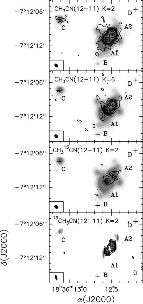
Figure 4: Overlay of the emission averaged in the velocity interval [105, 115] km s^-1of the CH₃CN (12–11) $K=2$, CH₃CN (12–11) $K=6$, CH${{}_{3}}^{13}$CN (12–11) K=2, and ¹³CH₃CN (12–11) $K=2$ transitions on the maps of continuum obtained with the SMA and PdBI (bottom panel) towards G24. Contour levels are 3, 6, 9, 12, 15, 20, 30, and 40 times $\sigma$, where 1$\sigma$ is 15 mJy beam^-1 for all species except for ¹³CH₃CN (12–11) for which 1$\sigma$ is 8 mJy beam^-1. The grayscale levels are the same as in Fig. 1. The crosses mark the positions of the sources identified by Furuya et al. (furuya02 (2002)) and Beltrán et al. (beltran04 (2004)). The synthesized beam is shown in the lower left corner.

3.2 CH₃CN and isotopologues

Figure 2 shows the spectra of the upper and lower SMA sideband around 230 and 220 GHz, respectively, obtained by integrating the emission inside the 3$\sigma$ contour level area towards G24 A1+A2, and G24 C. Figure 3 shows the PdBI spectrum around 214.3 GHz obtained by integrating the emission inside the 3$\sigma$ contour level area towards G24 A1 and A2. In Fig. 2, only the lines that have been analyzed are labeled. These are the lines with a good signal-to-noise and that could be unambiguously identified, i.e., that are not blended with other lines. As seen in these figures, altogether we detected 11 species (CO, HNCO, H₂¹³CO, SO, CH₃OH, HCOOCH₃, CH₂CO, CH₃CN, C₂H₅CN, OCS, ¹³CS), including 2 CO isotopologues (C¹⁸O and ¹³CO) and 2 CH₃CN isotopologues (CH${{}_{3}}^{13}$CN and ¹³CH₃CN).

Regarding the methyl cyanide emission, several $K$-components of CH₃CN (12–11) (up to $K$=8 for A1 and A2) are clearly detected towards G24 A1, A2, and C (Fig. 3). Several $K$-components of CH${{}_{3}}^{13}$CN and ¹³CH₃CN (12–11) (up to $K$=6) are also clearly detected towards G24 A1 and A2 (Figs. 2 and 3). Figure 3 shows only the $K$ = 0 to 4 components, which are those observed with the highest spectral resolution of 0.25 km s^-1. The ¹³CH₃CN (12–11) $K$ = 5 and 6 components, which have been observed with a spectral resolution of 3.5 km s^-1, have also been detected towards both cores G24 A1 and A2. Maps of the CH₃CN (12–11) emission averaged under the $K$ = 2 and 6 components, and of the CH${{}_{3}}^{13}$CN (12–11) and ¹³CH₃CN (12–11) emission averaged under the $K$ = 2 component towards G24 are shown in Fig. 4.

As seen in Fig. 4, the CH₃CN and isotopologues emission is clearly detected and resolved towards both cores A1 and A2. The emission peaks at the same position as the millimeter continuum.

3.3 Other high-density tracers

In addition to CH₃CN and isotopologues, most of the species detected towards G24 are high-density tracers. Figure 5 shows the emission averaged in the velocity interval (105–115) km s^-1 for the high-density tracers. The molecular outflow tracers are discussed in the next section. As seen in this figure, all the species have been clearly detected towards cores A1 and A2. All the species peak towards the millimeter continuum peaks. On the other hand, only CH₃OH, ¹³CS, HNCO, OCS, and H₂¹³CO have been detected towards core C, although in most cases the emission is so weak that it is not possible to distinguish any clear emission peak.

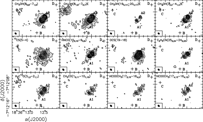
Figure 5: Images of the emission averaged in the velocity interval (105, 115) km s^-1for some observed molecular species towards G24. Contour levels are 3, 6, 9, 12, 15, 20, 30, and 40 times $\sigma$, where 1$\sigma$ is 15 mJy beam^-1 for all species except CH₃OH (8_1,8–7_0,7), ¹³CS (5–4), and OCS (19–18) for which 1$\sigma$ is 18 mJy beam^-1. The crosses mark the positions of the sources identified by Furuya et al. (furuya02 (2002)) and Beltrán et al. (beltran04 (2004)). The synthesized beam is shown in the lower left corner.

Figure 6: Combined SMA+IRAM 30-m channel maps of the ¹²CO (2–1) emission towards G24. The contour levels range from 0.35 to 7.35 Jy beam^-1 by steps of 1.4 Jy beam^-1 and from 7.35 to 18.55 Jy beam^-1 by steps of 2.8 Jy beam^-1. The cross indicates the phase reference center of the SMA observations. The synthesized beam is shown in the lower right corner of the last panel. The central velocity of each velocity interval is indicated in the upper left corner of each panel.

Figure 7: Same as Fig. 6 for the combined SMA+IRAM 30-m channel maps of the ¹³CO (2–1) line. The contour levels range from 0.35 to 11.55 Jy beam^-1 by steps of 1.4 Jy beam^-1

Figure 8: Blueshifted (blue contours) and redshifted (red contours) ¹²CO (2–1), ¹³CO (2–1), C¹⁸O (2–1), and SO (6₅–5₄) averaged emission overlaid on the SMA VEX 1.3 mm continuum emission (grayscale) towards G24. The maps have been reconstructed with a circular beam of 2^′′ to enhance the extended emission. The emission has been averaged in the velocity intervals (82, 97) km s^-1 (blueshifted emission) and (127, 142) km s^-1 (redshifted emission) for ¹²CO, (94, 103) km s^-1 (blueshifted emission) and (116, 127) km s^-1 (redshifted emission) for ¹³CO, (99, 104.4) km s^-1 (blueshifted emission) and (115.8, 122.4) km s^-1 (redshifted emission) for C¹⁸O, and (94, 104.2) km s^-1 (blueshifted emission) and (115.6, 124.6) km s^-1 (redshifted emission) for SO. Contour levels are 3, 6, 9, 12, 15, 20, 30, and 40 times 1$\sigma$, where 1$\sigma$ is 80 mJy beam^-1 for ¹²CO, 35 mJy beam^-1 for ¹³CO, 18 mJy beam^-1 for C¹⁸O, and 25 mJy beam^-1 SO. Grayscale contour for the continuum emission is 3$\sigma$, where 1$\sigma$ is 3.2 mJy beam^-1. The spectral line synthesized beam is shown in the lower left corner. The crosses mark the positions of the sources identified by Furuya et al. (furuya02 (2002)) and Beltrán et al. (beltran04 (2004)).

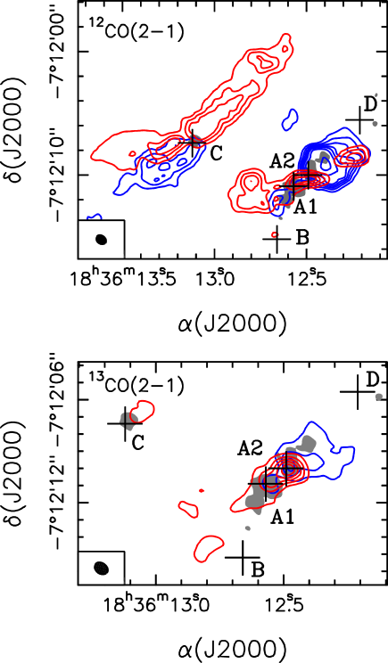
Figure 9: Blueshifted (blue contours) and redshifted (red contours) ¹²CO (2–1) (top panel) and ¹³CO (2–1) (bottom panel) averaged emission overlaid on the SMA VEX 1.3 mm continuum emission (grayscale) towards G24. The synthesized beam is $0\aas@@fstack{\prime\prime}86\times 0\aas@@fstack{\prime\prime}68$ at P.A.$=54\degr$ for ¹²CO and $0\aas@@fstack{\prime\prime}83\times 0\aas@@fstack{\prime\prime}64$ at P.A.$=55\degr$ for ¹³CO and is shown in the lower left corner. The emission has been averaged in the same velocity intervals as in Fig. 8. Contour levels are 3, 6, 9, 12, 15, 20, and 30 times 1$\sigma$, where 1$\sigma$ is 30 mJy beam^-1 for ¹²CO and ¹³CO. Grayscale contour for the continuum emission is 3$\sigma$, where 1$\sigma$ is 3.2 mJy beam^-1. The crosses mark the positions of the sources identified by Furuya et al. (furuya02 (2002)) and Beltrán et al. (beltran04 (2004)).

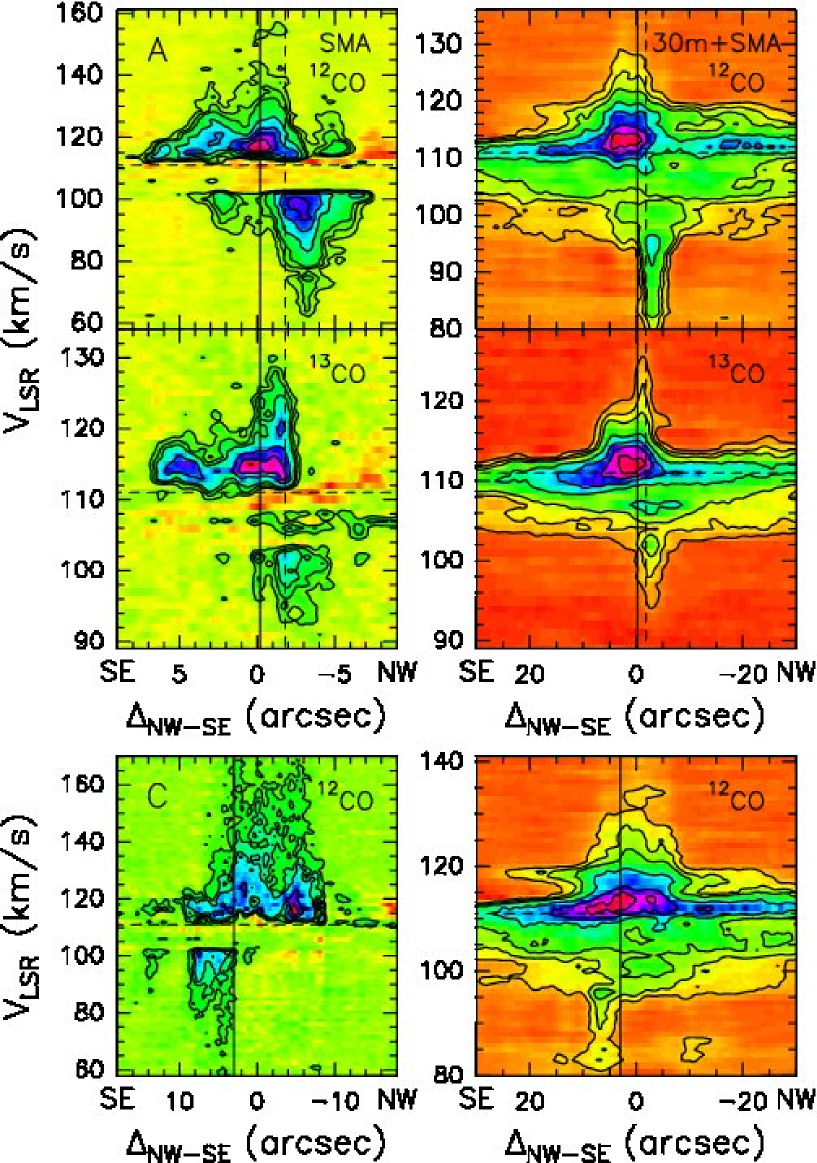
Figure 10: Position-velocity plots along the direction with P.A.=$-$40$\degr$ for outflow A (top and middle panels) and P.A.=$-$45$\degr$ for outflow C (bottom panels). The offsets are measured from the phase center, positive towards SE. Contour levels are 3$\sigma$, 6$\sigma$ 9$\sigma$ to 45$\sigma$ by steps of 6$\sigma$ where $\sigma$ is 0.033 Jy beam^-1 for ¹²CO SMA, 0.33 Jy beam^-1 for ¹²CO SMA+IRAM 30-m, 0.027 Jy beam^-1 for ¹³CO SMA, and 0.23 Jy beam^-1 for ¹³CO SMA+IRAM 30-m. The SMA maps have the highest angular resolution. (Top and middle panels) The vertical solid and dashed lines indicate the position of cores A1 and A2, respectively. The horizontal dashed line indicates the $V_{\rm LSR}$. (Bottom panels) The vertical solid line indicates the position of core C. The horizontal dashed line indicates the $V_{\rm LSR}$.

3.4 Molecular outflow tracers

The ¹²CO (1–0) emission towards G24 has been previously studied by Furuya et al. (furuya02 (2002)). These authors have discovered two bipolar molecular outflows in the region, oriented in the same direction, northwest-southeast: one associated with cores A1 and/or A2 and named outflow A, and the other one associated with core C and named outflow C. The cloud systemic velocity, $V_{\rm LSR}$, is 111 km s^-1(Furuya et al. furuya02 (2002)). As seen in Fig. 2, we have not only clearly detected ¹²CO (2–1) towards both cores, but also the CO isotopologues ¹³CO (2–1) and C¹⁸O (2–1), and SO (6₅–5₄). Figures 6 and 7 show the channel maps of the ¹²CO and ¹³CO (2–1) SMA+IRAM 30-m combined emission. Note that the extended emission seen in the ¹²CO (2–1) SMA+IRAM 30-m combined channel maps for velocities between 82 and 86 km s^-1 is due to a gas component along the line-of-sight. This component is not seen in ¹³CO. As seen in the channel maps, the outflow A is clearly seen in both tracers, while the outflow C is clearly visible in ¹²CO and only marginally in ¹³CO.

Figure 8 shows the ¹²CO, ¹³CO, C¹⁸O (2–1), and SO high-velocity blueshifted and redshifted averaged emission observed with the SMA. The maps shown in this figure have been reconstructed with a circular beam of 2^′′ to enhance the extended emission. As seen in this figure, the outflow A, which has a P.A.=140$\degr$, is clearly seen in all lines. On the other hand, the outflow C, which has a P.A.=145$\degr$, is clearly visible in ¹²CO and ¹³CO and just barely visible in C¹⁸O (2–1). The high-velocity SO (6₅–5₄) emission is hardly seen at redshifted velocities towards core C.

As seen in Fig. 8, the molecular outflow A shows a very prominent and poorly collimated blueshifted lobe and a more collimated redshifted lobe. This is especially visible in the higher angular resolution ¹²CO map visible in Fig. 9. The redshifted lobe shows an extension towards the northwest and the blueshifted one towards the southeast, especially in ¹²CO. The NW redshifted emission, detected at velocities close to the $V_{\rm LSR}$, is still clearly visible for velocities higher than 40 km s^-1 with respect to the $V_{\rm LSR}$. The redshifted NW emission can be seen in the position-velocity plots (Fig. 10) from about $-6^{\prime\prime}$ to $-4^{\prime\prime}$, and the blueshifted SE emission from about $1^{\prime\prime}$ to $3^{\prime\prime}$. A possible explanation for this blueshifted (redshifted) emission towards the redshifted (blueshifted) lobe of outflow A could be that outflow A is close to the plane of the sky. Alternatively, it could indicate the presence of a second outflow in this area.

The high-angular resolution maps (Fig. 9) and position-velocity plots (Fig. 10) seem to suggest that the core powering this molecular outflow is A2, because it is located closer to the geometrical center of the outflow. However, with these observations we cannot exclude the possibility of the existence of more than one outflow (see Sect. 4.3.1 for a more detailed discussion).

The molecular outflow C is highly collimated. This can be seen in the ¹²CO maps, either the 2^′′ resolution map or the high-angular resolution one. As clearly seen in Figs. 8, 9, and 15, the blueshifted lobe is much smaller than the redshifted one. This is particularly evident in the blueshifted emission maps averaged for high outflow velocities (not shown here), which we considered as those higher or lower than 36 km s^-1 with respect to the $V_{\rm LSR}$. For this high outflow-velocity range, the size of the blueshifted lobe is $\sim$3 times smaller than that of the redshifted lobe. Taking into account the fact that the molecular outflow consists of ambient gas that is swept up from a position close to where it is observed, a possible explanation for the morphology of the outflow C could be that the blueshifted lobe is close to the edge of the molecular cloud. That is, the blueshifted wind passes into a region where there is no, or little, molecular material to be swept up.

Another feature of the outflow C is the redshifted emission seen southeastern of core C. This redshifted emission is like a finger pointing towards the east, very prominent for outflow velocities close to the $V_{\rm LSR}$, but still visible for outflow velocities higher than 40 km s^-1 with respect to the $V_{\rm LSR}$. This feature has a length of $\sim$8$\aas@@fstack{\prime\prime}$4 ($\sim$0.31 pc). A possible explanation for this SE redshifted feature could be that the molecular outflow southwards of core C is interacting with the ambient cloud close to the position of the core. As a result of this interaction, the molecular outflow would be deflected towards the east and the emission would shift from blueshifted to redshifted. A similar scenario has been explained by Beltrán et al. (beltran02 (2002)) for the intermediate-mass outflow powered by IRAS 21391+5802 in terms of the shocked cloudlet model scenario, where an inverted bow shock is produced in the windward side of a dense ambient clump (Schwartz schwartz78 (1978)). This scenario could also explain the smaller size of the blueshifted lobe with respect to the redshifted one, because part of the material that would be entrained by the molecular outflow southwards of core C, would be deflected and redshifted. We have searched for a possible high-density southern clump responsible of the deflection of the outflow and have found a clump in CH₃OH (8_1,8–7_0,7)E at a position $\alpha$(J2000)=18^h 36^m 13$\aas@@fstack{\prime\prime}$09, $\delta$(J2000)=$-$07^h 12^m 7$\aas@@fstack{s}$7. However, the clump is only seen for redshifted velocities, $\sim$2–3 km s^-1 with respect to the $V_{\rm LSR}$, while one would expect the clump to be blueshifted like the southern lobe before deflection. Another possible explanation for the SE redshifted emission could be the presence of a second outflow, powered by a secondary source located close to core C but not resolved by our observations, but the blueshifted lobe would be missing.

Taking the blueshifted and redshifted emission into account, the total extent of the outflows is $\sim$$13\aas@@fstack{\prime\prime}5$ ($\sim$0.5 pc) for outflow A and $\sim$$15\aas@@fstack{\prime\prime}2$ ($\sim$0.57 pc) for outflow C.

Figure 11: Rotation diagram for cores A1, A1b, A1c, and A2 in G24 with superimposed fit. Open circles and filled triangles correspond to the ¹³CH₃CN (12–11) and the CH₃CN (12–11) $v_{8}=1$ transitions, respectively.

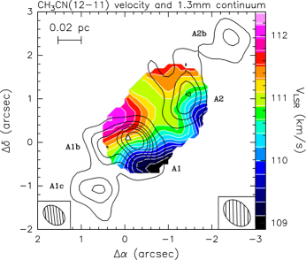
Figure 12: Overlay of the map of the 1.3 mm continuum emission obtained with the very extended SMA configuration (contours) on that of the CH₃CN (12–11) line velocity (colour scale). Contour levels are the same as in Fig. 1. Offsets are measured with respect to the phase center. The triangle marks the position of the HC Hii region in G24 A1 (Beltrán et al. beltran07 (2007)). The synthesized beam of the continuum (line) emission is shown in the lower left (right) corner.

4 Analysis and Discussion

4.1 Temperature and mass estimates

CH₃CN is a symmetric top molecule, so it can be used to estimate the temperature in the cores. The rotational temperature, $T_{\rm rot}$, and the total methyl cyanide column density, $N_{\rm CH_{3}CN}$, can be estimated by means of the rotation diagram method, which assumes that the molecular levels are populated according to LTE conditions at a single temperature $T_{\rm rot}$. In the high-density limit where level populations are thermalized, one expects that $T_{\rm rot}=T_{\rm kin}$, the kinetic temperature. The CH₃CN ground-level transitions appear to be optically thick for all cores, as suggested by the ratio between the main species and isotopologues. Therefore, the Boltzmann plot was only performed using the ¹³CH₃CN and vibrational excited CH₃CN transitions (see Fig. 11). The core A1c has not been detected in ¹³CH₃CN and only marginally in CH${{}_{3}}^{13}$CN. Therefore, the rotation diagram in Fig. 11 has been calculated with only three measurements, one corresponding to CH${{}_{3}}^{13}$CN $K$=2, and two corresponding to CH₃CN $v_{8}=1$, ($K,l$)=(3,$-1$) and ($K,l$)=(6,$+1$). The $T_{\rm rot}$ estimated for this core is 146 K, and $N_{\rm CH_{3}CN}$ is about 1$\times$10¹⁶ cm^-2. The relative abundance [CH₃CN]/[¹³CH₃CN] was estimated to be 46 following Wilson & Rood (wilson94 (1994)) for a galactocentric distance of 3.7 kpc. The temperatures and column densities obtained are consistent with those estimated by Beltrán et al. (beltran05 (2005)) from CH${{}_{3}}^{13}$CN (12–11) and (5–4), and CH₃CN (5–4) $v_{8}=1$.

The masses of the individual cores, which are given in Table 2, have been estimated from the 1.3 mm dust continuum emission observed with the SMA at the highest angular resolution (VEX) assuming a dust opacity of $\simeq 0.8$ cm² g^-1 at 1.3 mm (Ossenkopf & Henning ossen94 (1994)), a gas-to-dust ratio of 100, and a dust temperature equal to $T_{\rm rot}$. For the three cores for which an estimate of $T_{\rm rot}$ is not possible with the rotation diagram, a range of masses is given assuming that the dust temperature of the cores ranges from 30 to 60 K. The lower value is the kinetic temperature of $\sim$30 K estimated from ammonia observations carried out with the Very Large Array (VLA) by Codella et al. (codella97 (1997)) towards G24. However, taking into account that CH₃CN has been detected towards core C (Fig. 4), we expect that the temperature, at least for this core, is higher. In Table 2 we also give the masses estimated from the compact plus VEX configuration SMA map. In this case, the emission of some individual cores cannot be resolved, and therefore, the masses correspond to that of cores A1+A1b+A1c and A2+A2b.

4.2 Dense gas kinematics

Following Beltrán et al. (beltran04 (2004), beltran05 (2005), beltran11 (2011)), the velocity field of the cores has been studied thanks to the CH₃CN and isotopologues emission.

4.2.1 Velocity gradients

Figure 12 shows the map of the CH₃CN line velocity for the G24 A1 and A2 cores overlaid on the VEX continuum emission. The line velocity map has been obtained by simultaneously fitting the CH₃CN $K=0$,1,2,3, and 4 components, assuming identical line widths and fixing their separations to the laboratory values, at each position where CH₃CN is detected. The validity of the assumption of identical line widths has been checked by fitting separately different $K$-components. Beltrán et al. (beltran05 (2005)) calculated very small variations in the CH₃CN (12–11) line widths from $K=0$ to 6 (see their Table 7). As seen in Fig. 12, we have clearly detected the same velocity gradients in the southwest-northeast direction observed by Beltrán et al. (beltran04 (2004)) towards G24 A1 and A2.

The continuum emission of core A1 peaks at the center of the southern velocity gradient, which is very close to the position of the HC Hii region. The P.A. of this velocity gradient is about 50$\degr$. The velocity shift measured over an extent of $\sim$13000 AU is $\sim$3.4 km s^-1, that is, a velocity gradient of about 54 km s^-1 pc^-1. The peak of the continuum emission of core A2 is close to the center of the northern velocity gradient, which has a P.A. of $\sim$40$\degr$. The velocity shift measured over an extent of $\sim$11500 AU is $\sim$2.4 km s^-1, that is, a velocity gradient of about 43 km s^-1 pc^-1.

Unfortunately our data do not have enough sensitivity to allow us to properly map the velocity field towards the core C and better constrain the direction of the velocity gradient detected in CS (3–2) by Beltrán et al. (beltran04 (2004)).

4.2.2 Multiple components towards G24 A1

The analysis of ¹³CH₃CN (12–11) has clearly revealed the existence of 2 velocity components towards core A1. This is clearly seen in Fig. 3 for $K$=3 and 4. The second velocity component is less evident for $K$=1 because it is blended with $K$=0, and for $K$=2 because it is blended with some species typical of hot cores, such as dimethyl ether (CH₃OCH₃) and/or methyl formate (CH₃OCHO). On the other hand, the $K$=0 transition is very close to the edge of the observed band, which makes it very difficult to distinguish the second velocity component. The 2 velocity components can also be seen in CH${{}_{3}}^{13}$CN and C₂H₅CN as shown in Fig. 13, where we show the spectra averaged over the core towards A1 and A2. Note that the reason for showing CH${{}_{3}}^{13}$CN (12–11) $K$=2 instead of $K$=3 is due to the fact that the latter one is blended with CH₃CN (12–11) $K$=6.

Figure 13: (Top panels) ¹³CH₃CN (12–11) $K$=3 (black line), CH${{}_{3}}^{13}$CN (12–11) $K$=2 (dotted line), and C₂H₅CN (25_2,24–24_2,23) (gray line) obtained by integrating the emission inside the 3$\sigma$ contour level area towards G24 A1 (left) and A2 (right). The vertical solid line indicates the $V_{\rm LSR}$. (Bottom panels) Overlay of the averaged emission in the velocity interval (105, 107.5) km s^-1(component 1; left) and (108.75, 114.25) km s^-1(component 2; right) of the ¹³CH₃CN (12–11) $K=3$ transition on the map of the 1.4 mm continuum emission obtained with the PdBI towards G24 A1 and A2. Contour levels are the same as in Fig. 1. The grayscale levels are 3, 6, 9, 12, 15, 20, and 30 times $\sigma$, where 1$\sigma$ is 3.7 mJy beam^-1 for component 1, and 7.2 mJy beam^-1 for component 2. The black triangle marks the position of the HC Hii region in G24 A1 (Beltrán et al. beltran07 (2007)). The synthesized beam is shown in the lower right corner.

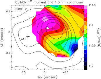
Figure 14: Overlay of the map of the 1.3 mm continuum emission obtained with the very extended SMA configuration (contours) on the map of the first moment of the C₂H₅CN (25_2,24–24_2,23) second velocity component (colour scale). Contour levels are the same as in Fig. 1. Offsets are measured with respect to the phase center. The triangle marks the position of the HC Hii region in G24 A1 (Beltrán et al. beltran07 (2007)) and the crosses the position of sources A1 and A1b.

As seen in Fig. 13, the spectra towards A1 clearly show 2 components. Component 1 that peaks at about 106 km s^-1 (107 km s^-1 for C₂H₅CN), and component 2 that peaks at about 111 km s^-1 (the systemic velocity). The spectra towards A2 do not show an apparent component peaking at a velocity of $\sim$106 km s^-1, although they do show a significant blueshifted wing. The bottom panels in Fig. 13 show the ¹³CH₃CN (12–11) $K=3$ emission averaged for a velocity interval (105, 107.5) km s^-1, corresponding to component 1, and (108.75, 114.25) km s^-1, corresponding to component 2. As seen in these maps, the 2 components peak at a different position. Component 1 peaks towards the southwest of the core A1 continuum emission peak, and its emission is clearly elongated in the SW direction. On the other hand, the emission peak of component 2 coincides with that of the core A1 continuum emission and with the position of the HC Hii region. For core A2, the peak of the emission averaged for the 2 velocity intervals is similar although not coincident, and in both cases is displaced from the position of the continuum emission peak. A SW elongation is also visible for component 1, but not for component 2. Hence, we cannot discard a priori the existence of 2 velocity components also for core A2.

We have searched for the two different velocity components in the other high-density tracers observed with the SMA, and in particular in CH₃CN and CH₃CN $v_{8}$=1. However, although the spectral resolution of the observations is enough to disentangle the emission of the two components, what we have found is a significant blueshifted wing in some cases, but not two clearly separated components. We have reconstructed the PdBI ¹³CH₃CN $K$=3 and the SMA CH₃CN $K$=3 maps with the same synthesized beam of $0\aas@@fstack{\prime\prime}89\times 0\aas@@fstack{\prime\prime}0.59$ P.A.=10$\degr$, i.e. a beam encompassing the beams of the SMA and PdBI maps, and have recalculated the spectrum towards A1. The component 1 was still clearly visible in ¹³CH₃CN, even after degrading the spectral resolution to that of the SMA observations (0.6 km s^-1), and in CH${{}_{3}}^{13}$CN. On the other hand, the component 1 was still not evident in the CH₃CN  spectrum.

Table 3: Properties of the molecular outflows^a,b

	$R^{c}\,\cos\leavevmode\nobreak\ i$	$M_{\rm out}$	$\dot{M}_{\rm out}\,\tan\leavevmode\nobreak\ i$	$P^{d}\,\sin\leavevmode\nobreak\ i$	$E^{d}\,\sin^{2}\leavevmode\nobreak\ i$	$F^{d}\,\sin^{2}\leavevmode\nobreak\ i/\cos\leavevmode\nobreak\ i$	$t_{\rm out}\,\cot\leavevmode\nobreak\ i$
Outflow	(pc)	($M_{\odot}$)	($M_{\odot}$ yr-1)	($M_{\odot}$ km s-1)	($10^{46}$ erg)	($M_{\odot}\,\mbox{km s}^{-1}$ yr-1)	(yr)
A	0.50	27.3	$1.5\times 10^{-3}$	245	2.5	$1.4\times 10^{-2}$	$1.8\times 10^{4}$
Ce	0.57	7.3	$3.0\times 10^{-4}$	62	0.6	$2.6\times 10^{-3}$	$2.4\times 10^{4}$
C red fingerf	0.31	4.2	$2.2\times 10^{-4}$	33	0.3	$1.7\times 10^{-3}$	$1.9\times 10^{4}$

(a) The tabkle indicates the estimated values. In case of knowing the inclination angle with respect to the plane of the sky, $i$, of the outflows, the parameters should be corrected accordingly.
(b) The blueshifted emission has been integrated for the velocity range (94, 103) km s^-1, and the redshifted one for (116, 127) km s^-1.
(c) Total size of the lobes.
(d) Momenta and kinetic energies are calculated relative to the cloud velocity.
(e) The redshifted emission seen SE of core C has not been taken into account in the calculations.
(f) Redshifted emission seen SE of core C.

We have studied the velocity field of the 2 components in ¹³CH₃CN towards A1 to see whether the presence of another velocity component at $\sim$106 km s^-1 could be responsible for the SW–NE velocity gradient seen in CH₃CN towards core A1 (see Fig. 12). In fact, a velocity gradient might also be mimicked by two distinct cores with different $V_{\rm LSR}$ that are too close to be resolved by our observations. Figure 14 shows the first moment map of C₂H₅CN computed over a velocity interval from 108.5 to 114.5 km s^-1, that is, over the range of the second velocity component. We have analyzed the velocity field of C₂H₅CN, because this is the high-density tracer with 2 components clearly distinguishable that shows the strongest emission towards G24 A1 (see Fig. 13). The analysis indicates that component 2 shows a velocity gradient similar to the one observed in CH₃CN, centered close to the position of the continuum emission peak and the HC Hii region, although with a velocity range slightly smaller ($\sim$109.9–111.4 km s^-1). Therefore, we conclude that the velocity gradient seen towards core A1, first detected in CH₃CN by Beltrán et al. (beltran04 (2004)), could only be marginally affected by the presence of a second core at a different $V_{\rm LSR}$, and is produced by a structure rotating around the star powering the HC Hii region. Hence, the velocity component at $\sim$106 km s^-1 would not be related to this gradient. The presence of a SW core is also discarded by the fact that a secondary continuum emission peak is not detected in that direction (Fig. 13). One would expect that any embedded core should be better detected in continuum than in line emission.

4.3 The molecular outflows

Figures 8 and 9 show the molecular outflows A and C mapped in ¹²CO (2–1), ¹³CO (2–1), C¹⁸O (2–1), and SO (6₅–5₄) towards G24. In Fig. 10 we show the position-velocity plots along the outflows A and C. For the sake of completeness we show both the SMA and the combined SMA+IRAM 30-m data. The outflow C is hardly visible in ¹³CO (2–1) with the SMA at a resolution of $\sim$0$\aas@@fstack{\prime\prime}$7, and hence, for this outflow we show only the ¹²CO (2–1) data. Note that the cuts were made along P.A.=$-$40° (outflow A) and P.A.=$-$45° (outflow C) and all the plots have been obtained after averaging the emission along the direction perpendicular to the cut with the purpose of increasing the S/N of the plots.

4.3.1 Which source is powering outflow A?

One of the questions that still remains open in the study of G24 is which core, A1 or A2 (or both), is driving outflow A. The high-angular resolution maps (Fig. 9) seem to indicate that the core powering this outflow is A2, because it is located closer to the geometrical center of the outflow. This is especially visible in the ¹³CO map, where outflow A shows a clear bipolarity centered in core A2. However, the most clear evidence that A2 is the powering source comes from the position-velocity plots along the outflow (Fig. 10). In these plots the vertical solid and dashed lines indicate the position of core A1 and A2, respectively. As can be seen in these plots, core A2 is located at the position where the emission, or the emission at the highest outflow velocity, changes from being blueshifted to redshifted. This is more evident in the ¹³CO SMA plots, because no redshifted emission is detected at any position before that of core A2. Regarding core A1, the position-velocity plots seem to indicate that this core is not powering any outflow. However, as shown in Fig. 9, the CO emission is very complex towards cores A1 and A2, with redshifted emission towards the blueshifted lobe and the opposite. Hence, we cannot totally discard the possibility that core A1 could be powering an additional outflow in the region. In any case, this possible outflow would not be the most prominent one, which, as already mentioned, is driven by core A2.

4.3.2 Physical parameters

Table 3 gives the parameters of outflows A and C, as well as those of the redshifted emission feature seen SE of core C. The emission of this feature has not been taken into account when calculating the parameters of outflow C. The parameters have not been corrected for inclination angle, $i$, of the flow with respect to the plane of the sky. However, we have indicated in Table 3 the correction for the inclination to be applied for each outflow parameter. The size of the lobes, mass $M_{\rm out}$, outflow mass loss rate $\dot{M}_{\rm out}$, momentum $P$, kinetic energy $E$, momentum rate in the outflows $F$, and dynamical timescale $t_{\rm out}$ were derived from the ¹³CO emission for the velocity ranges indicated in Table 3. The ¹³CO channel maps used were those reconstructed with a 2^′′ circular beam. The dynamical timescale of the blueshifted and redshifted lobes was estimated as $t_{\rm out}=R/V_{\rm out}$, where $V_{\rm out}$ is the difference in absolute value between the maximum blueshifted or redshifted velocity and the systemic velocity, $V_{\rm LSR}$=111 km s^-1. The $t_{\rm out}$ of the outflow is the maximum dynamical timescale of the two lobes. The parameters $R$, $M_{\rm out}$, $P$, and $E$ were calculated for the blueshifted and redshifted lobes separately, and then added to obtain the total value. The [¹³CO]/[H₂] abundance ratio of $2.2\times 10^{-6}$ was estimated following Wilson and Rood (wilson94 (1994)), and assuming an [H₂]/[CO] abundance ratio of 10⁴ (e.g. Scoville et al. scoville86 (1986)). The excitation temperature, $T_{ex}$, was estimated from the SMA+IRAM 30m ¹²CO peak brightness temperature, $T_{\rm B}$, of the averaged blueshifted and redshifted emission of the outflows separately, assuming that $T_{\rm B}$=$J(T_{ex})$–$J(T_{\rm BG})$, where the background temperature $T_{\rm BG}$ is 2.7 K. The $T_{ex}$ values are in the range 40–50 K.

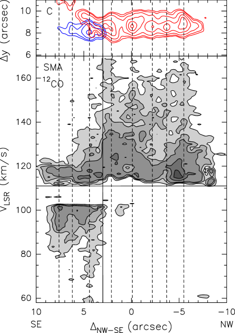
Figure 15: (Top panel) Blueshifted (blue contours) and redshifted (red contours) ¹²CO (2–1) averaged emission towards G24 C. The emission has been averaged in the velocity intervals (58, 74.5) km s^-1 (blueshifted emission) and (148, 167.5) km s^-1 (redshifted emission). The molecular outflow map has been rotated $-$45$\degr$. The offsets are measured from the phase center, positive towards SE. Contour levels are 3, 4, 6, 9, and 12 times 1$\sigma$, where 1$\sigma$ is 15 mJy beam^-1 (12 mJy) for the blueshifted (redshifted) emission. (Bottom panel) Same as bottom left panel of Fig. 10. The vertical and horizontal solid lines indicate the position of core C and the $V_{\rm LSR}$, respectively. The position of each knot along the outflow axis is marked with a vertical dashed line.

As seen in Table 3, the values of $M_{\rm out}$, $\dot{M}_{\rm out}$, $P$, $E$, and $F$ of outflow A are about 4–5 times higher than those of outflow C. On the other hand, the size of the outflow C is larger and the dynamical timescales are comparable. Even if we add the redshifted SE feature to the calculations of outflow C, the values estimated are still smaller than those of outflow A. This suggests that outflow C is less massive and powerful, probably because it is powered by a less massive and luminous source. In fact, following the correlations between the outflow parameters and the bolometric luminosity of the powering source, $L_{\rm bol}$, found by López-Sepulcre et al. (lopez09 (2009)) for a sample of high-mass star-forming regions, the source powering outflow A should have a $L_{\rm bol}$ of a few 10⁴–10${}^{5}\,L_{\odot}$, while the one driving outflow C should have a $L_{\rm bol}$ of a few 10³–10${}^{4}\,L_{\odot}$. Furuya et al. (furuya02 (2002)) estimated a size of the lobes almost twice the size estimated with our observations. The fact that the synthesized beam of their observations was $\sim$$4\aas@@fstack{\prime\prime}5$, made them more sensitive to extended emission than ours. The $M_{\rm out}$ and $\dot{M}_{\rm out}$ estimates obtained by Furuya et al. (furuya02 (2002)) for outflow A are three times smaller than ours, while for outflow C their values are quite similar to ours. The dynamical timescales are comparable.

4.3.3 Episodic outflow

One of the striking features about the morphology of outflow C is its clumpy structure. This is particularly visible in Fig. 15, where we show the blueshifted and redshifted emission maps averaged for high outflow velocities. As seen in this figure, the outflow lobes, in particular the redshifted one, show discrete knots. The knotty appearance of the outflow with multiple clumps aligned along the flow axis resembles that of the high-mass outflow HH 80–81 (Qiu & Zhang qiu09 (2009)), where a series of CO bullets have been discovered. These authors propose that the bullets have not been created in situ from entrained or swept-up ambient medium, but are the result of episodic, disk-mediated accretion. For outflow C, the morphology could be explained in terms of an episodic outflow where the knots are made of swept-up ambient gas. In fact, in the position-velocity plot along the axis of this outflow, there is an increase in the extreme emission velocity at the position of all the knots for the lowest emission contour level. According to Arce & Goodman (2001b ), the velocity structure at the position of the knots is characteristic of the prompt entrainment mechanism, which will produce the highest velocities at the position of the local CO maximum, and decreasing velocity trend towards the source. The fact that the maximum outflow velocity does not increase linearly as a function of distance from the powering source (Fig. 15) indicates that there is a different “Hubble law” associated with each knot, corresponding with each mass-ejection episode. The extreme emission velocity for each mass-ejection episode will not necessarily be the same. This is because not all the outburst from an episodic source will necessarily have the same angle with respect to the plane of the sky or will accelerate the ambient gas to the same maximum velocity (Arce & Goodman 2001a ).

5 Conclusions

We analyzed millimeter data obtained with the SMA and the IRAM PdBI interferometers, and the IRAM 30-m telescope of the dust and gas emission towards the cores in the high-mass star-forming region G24.78+0.08. The synthesized beam of $<1^{\prime\prime}$ of the observations has allowed us to study with unprecedented high-angular resolution the structure and the velocity field of the cores, and the molecular outflows powered by the YSOs embedded in the HMCs.

The millimeter continuum emission towards the cores A1 and A2 has been resolved into additional cores. Core A1 has been resolved into 3 cores named A1, A1b, and A1c, whereas core A2 has been resolved into 2 named A2 and A2b. Interestingly, the cores are aligned in a southeast-northwest direction coincident with that of the molecular outflows detected in the region. This suggests a preferential direction for star formation in this region that could possibly depend on the direction of the magnetic field. It could also indicate star formation in filaments or sheets. The core associated with the HC Hii region is A1. The masses of the cores for which it has been possible to estimate the rotational temperature range from 7 to 22 $M_{\odot}$. The rotational temperatures range from 128 to 180 K.

The velocity gradients towards cores A1 and A2, first detected by Beltrán et al. (beltran04 (2004)) in CH₃CN (12–11), have been confirmed by the new SMA observations. Unfortunately, the sensitivity of the observations have not allowed us to better constrain the direction of the velocity gradient detected in CS (3–2) by Beltrán et al. (beltran04 (2004)).

The CH${{}_{3}}^{13}$CN, ¹³CH₃CN and C₂H₅CN observations have revealed the existence of 2 velocity components towards A1. The component at $\sim$111 km s^-1 is associated with the velocity gradient seen in CH₃CN and peaks close to the position of the millimeter continuum peak and of the HC Hii region. The component at $\sim$106 km s^-1 peaks towards the SW of core A1 and does not seem to be associated with a millimeter continuum emission peak.

The two molecular outflows in the region have been mapped in different tracers. The position-velocity plots along outflow A and the ¹³CO (2–1) averaged blueshifted and redshifted emission indicate that this outflow is driven by core A2. Regarding core A1, the position-velocity plots seem to indicate that this core is not powering any outflow. However, due to the fact that the outflow structure is very complex towards cores A1 and A2, we cannot totally discard the possibility that core A1 could be powering an additional outflow in the region. The outflow C is highly collimated and clumpy. The clumpiness and the ¹²CO (2–1) position-velocity plot suggest that this outflow could be episodic, and that the outflow clumps are made of swept-up ambient gas.

- (1) Arce, H. G., & Goodman, A. A. 2001, ApJ, 551, L171
- (2) Arce, H. G., & Goodman, A. A. 2001, ApJ, 554, 132
- (3) Beltrán, M. T., Cesaroni, R., Codella, C. et al. 2006, Nature, 443, 427
- (4) Beltrán, M. T., Cesaroni, R., Moscadelli, L., & Codella, C. 2007, A&A, 471, L13
- (5) Beltrán, M. T., Cesaroni, R., Neri, R. et al. 2004, ApJ, 601, L187
- (6) Beltrán, M. T., Cesaroni, R., Neri, R. et al. 2005, A&A, 435, 901
- (7) Beltrán, M. T., Cesaroni, R., Neri, R., & Codella, C. 2011, A&A, 525, 151
- (8) Beltrán, M. T., Girart, J. M., Estalella, R., Ho, P. T. P., & Palau, A. 2002, ApJ, 573, 246
- (9) Beuther, H., Schilke, P., Sridharan, T. K. et al. 2002, A&A, 383, 892
- (10) Briggs, D. 1995, Ph.D. Thesis, New Mexico Inst. Mining & Tech.
- (11) Cesaroni, R., Galli, D., Lodato, G. et al. 2007, in Protostars & Planets V, eds. B. Reipurth, D. Jewitt, & K. Keil (University of Arizona Press), 197
- (12) Cesaroni, R., Neri, R., Olmi, L. et al. 2005, A&A, 434, 1039
- (13) Cesaroni, R., Codella, C., Furuya, R. S., & Testi, L. 2003, A&A, 401, 227
- (14) Codella, C., Testi, L., & Cesaroni, R. 1997, A&A, 325, 282
- (15) Furuya, R. S., Cesaroni, R., Codella, C. et al. 2002, A&A, 390, L1
- (16) Galván-Madrid, R., Rodríguez, L. F., Ho, P. T. P., & Keto, E. 2008, ApJ, 674, L33
- (17) Ho, P. T. P., Moran, J. M., & Lo, K. Y. 2004, ApJ, 616, L1
- (18) Keto, E. 2002, ApJ, 568, 754
- (19) Keto, E. R., Ho, P. T. P., & Haschick, A. D. 1987, ApJ, 318, 712
- (20) Keto, E., & Zhang, Q. 2010, MNRAS, 406, 102
- (21) Krumholz, M. R., Klein, R. I., McKee, C. F., Offner, S. S. R., & Cunningham, A. J. 2009, Science, 323, 754
- (22) Longmore, S. N., Burton, M. G., Keto, E., Kurtz, S., & Walsh, A. J. 2009, MNRAS, 399, 861
- (23) López-Sepulcre, A., Codella, C., Cesaroni, R. et al. 2009, A&A, 499, 811
- (24) Moscadelli, L., Goddi, C., Cesaroni, R., Beltrán, M. T., & Furuya, R. S. 2007, A&A, 472, 867
- (25) Ossenkopf, V., & Henning, Th. 1994, A&A, 291, 943
- (26) Peters, T., Banerjee, R., Klessen, R. S., Mac Low, M.-M., Galván-Madrid, R., & Keto, E. 2010, ApJ, 711, 1017
- (27) Qiu, K., & Zhang, Q. 2009, ApJ, 702, L66
- (28) Sault, R. J., Teuben, P. J., & Wright, M. C. H. 1995, in ASP Conf. Ser. 77: Astronomical Data Analysis Software and Systems IV, 433
- (29) Scoville, N. Z., Sargent, A. I., Sanders, D. B. et al. 1986, ApJ, 303, 416
- (30) Schwartz, R. D. 1978, ApJ, 223, 884
- (31) Shepherd, D. S., & Churchwell, E. 1996a, 457, 267
- (32) Shepherd, D. S., & Churchwell, E. 1996b, 472, 225
- (33) Vig, S., Cesaroni, R., Testi, L., Beltrán, M. T., & Codella, C. 2008, A&A, 488, 605
- (34) Wilson, T. L., & Rood, R. T. 1994, ARA&A, 86, 317
- (35) Zhang, Q., & Ho, P. T. P., & Ohashi, N. 1998, ApJ, 494, 636
- (36) Zhang, Q., Hunter, T. R., Brand, J., Sridharan, T. K. et al. 2001, ApJ, 552, 167