Decay rates for topological memories encoded with Majorana fermions

Abstract

Recently there have been numerous proposals to create Majorana zero modes in solid state heterojunctions, superconducting wires and optical lattices. Putatively the information stored in qubits constructed from these modes is protected from various forms of decoherence. Here we present a generic method to study the effect of external perturbations on these modes. We focus on the case where there are no interactions between different Majorana modes either directly or through intermediary fermions. To quantify the rate of loss of the information stored in the Majorana modes we study the two-time correlators for qubits built from them. We analyze a generic gapped fermionic environment (bath) interacting via tunneling with different components of the qubit (different Majorana modes). We present examples with both static and dynamic perturbations (noise), and using our formalism we derive a rate of information loss, for Majorana memories, that depends on the spectral density of both the noise and the fermionic bath.

I Introduction

Topological quantum computation requires the existence of topologically ordered states whose low energy excitations follow non-Abelian statistics. The subspace of states corresponding to a fixed number of quasiparticles is degenerate, to an exponential precision, in the separation between quasiparticles, and an exchange of the positions of these anyonic excitations, also known as braiding, leads to a unitary transformation within this low energy subspace. These unitary operations are insensitive to the exact path used to perform the braiding operation and in many cases, for an appropriate encoding, braiding operations correspond to “standard” one- and two-qubit gates within the low energy subspace. These operations can be used as building blocks for fault tolerant quantum computation.

There are many candidate systems for experimental realizations of topological phases of matter with these properties. There is preliminary evidence that the $\nu=5/2$ fractional quantum Hall state may have non-Abelian excitations key-23 ; key-24 ; key-25 . Spin-triplet $p_{x}+ip_{y}$ pairing superfluidity occurs in the A-phase of $\mathrm{{}^{3}He}$ key-26 ; key-27 and in strontium ruthenates key-28 ; key-29 ; key-30 ; key-31 ; key-32 ; key-83 , in which half quantum vortices would be non-Abelian key-33 ; key-3 . There are also proposals to realize chiral p-wave superconductors in ultra-cold atom systems key-21 ; key-35 ; key-34 . Furthermore there have been many advances towards producing topological states of matter in layered heterojunction systems key-36 ; key-37 ; key-38 ; key-15 ; key-2 ; key-4 ; key-5 ; key-7 ; key-8 ; key-16 ; key-17 ; key-18 ; key-20 ; key-6 .

Virtually all current experimentally viable proposals for platforms for topological quantum computation only support Ising type anyons which are carried by Majorana fermion modes. Colloquially speaking these fermions are half of a regular fermion. More precisely they are self-adjoint operators $\gamma_{i}$ which can be written as a sum of an annihilation and creation operator for one fermion mode and which satisfy the algebra:

$$\left\{\gamma_{i},\,\gamma_{j}\right\}=2\delta_{ij},\,\gamma_{i}^{\dagger}=\gamma_{i}$$ (1)

Any two Majorana fermion operators can be combined into a regular fermion mode $c$ and its adjoint $c^{\dagger}$ via $c=\frac{1}{2}\left(\gamma_{1}+i\gamma_{2}\right)$ and $c^{\dagger}=\frac{1}{2}\left(\gamma_{1}-i\gamma_{2}\right)$.

The topological qubit is made up of four spin polarized MBSs $\gamma_{1},\,\gamma_{2},\,\gamma_{3}$ and $\gamma_{4}$ key-43 . These can be combined into two sets of creation and annihilation operators:

$$\begin{array}[]{rcl}c_{1}&=&\frac{1}{2}\left(\gamma_{1}+i\gamma_{2}\right)\end{array} \begin{array}[]{rcl}c_{1}^{\dagger}&=&\frac{1}{2}\left(\gamma_{1}-i\gamma_{2}\right)\end{array}$$ (4)

$$\begin{array}[]{rcl}c_{2}&=&\frac{1}{2}\left(\gamma_{3}+i\gamma_{4}\right)\end{array} \begin{array}[]{rcl}c_{2}^{\dagger}&=&\frac{1}{2}\left(\gamma_{3}-i\gamma_{4}\right)\end{array}$$ (7)

For the logical basis it is convenient to work in the even fermion parity subspace. The qubit basis can be chosen to be $\left|+_{L}\right\rangle\equiv\left|00\right\rangle$ and $\left|-_{L}\right\rangle\equiv\left|11\right\rangle$ where the $0$’s and $1$’s refer to the occupation numbers relative to the complex fermion operators in Eq. (4). Because of fermion parity conservation, any operation that does not entangle the states with the environment cannot mix even and odd fermion parity states for the qubits. As such, all gates acting on the topological qubit should not take the system out of the logical subspace. Furthermore all the operators of the single spin Clifford group may be produced by braiding the four vortices of our qubit leading to potentially topologically protected gates key-14 . In particular the various single qubit operations in our logic basis may be conveniently written in terms of the Majorana operators. For future use we note that in this encoding

$$\sigma^{z}=-i\gamma_{1}\gamma_{2},\;\sigma^{x}=-i\gamma_{2}\gamma_{3},\;\sigma^{y}=i\gamma_{1}\gamma_{3}.$$ (8)

Here all the sigma matrices are with respect to the logic basis $\left|+_{L}\right\rangle$ and $\left|-_{L}\right\rangle$. We will primarily be interested in correlators of the form $\left\langle\sigma^{\mathrm{z}}\left(0\right)\sigma^{\mathrm{z}}\left(\mathrm{T}\right)\right\rangle=-\left\langle\gamma_{1}\left(0\right)\gamma_{2}\left(0\right)\gamma_{1}\left(\mathrm{T}\right)\gamma_{2}\left(\mathrm{T}\right)\right\rangle$. We will proceed to calculate these below.

The Majorana operators are zero modes of some mean field Hamiltonian $\left[{H}_{\mathrm{MF}},\,\gamma_{i}\right]=0$ so it can be argued that these modes are protected from decoherence as the mean field Hamiltonian when restricted to the subspace generated by these modes is zero. One of the open tasks of topological quantum computation is associated with understanding the extent of this protection. This is the subject of this paper.

II Summary of main ideas

In this section we outline the setup of the rest of the paper. We present the relevant Hamiltonian and discuss its basic properties. We describe the type of qubit we will focus on in the text, a localized Majorana mode, and give an overview of some other encodings we shall not consider in this paper. We describe the kinds of calculations of memory coherence we are going to do in this paper. We also give a Section by Section outline.

We begin our discussion with relevant Hamiltonians. The Majorana fermions interact with the external environment via tunneling type Hamiltonians. On symmetry grounds, for a single Majorana mode, any such interaction may be written as:

$${H_{\mathrm{int}}}=\gamma\int{d^{d}r\left[u_{0}(\vec{r})\,\Phi^{\dagger}\left(\vec{r}\right)\Psi^{\dagger}\left(\vec{r}\right)-u_{0}^{*}(\vec{r})\,\Psi\left(\vec{r}\right)\Phi\left(\vec{r}\right)\right]}.$$ (9)

Here $u_{0}(\vec{r})$ is the localized mode function associated with the Majorana bound state, $\Phi(\vec{r})$ is any local bosonic field, which in the simplest case is a tunneling amplitude (complex number) and $\Psi(\vec{r})$ is a regular (complex) fermion field. In this paper we will analyze multiple Majorana fermions coupled to different types of environments via Hamiltonians of the form given in Eq. (9). Furthermore the fermions in the bath will always be assumed to be gapped, for example, electrons in an insulating or superconducting material (environments composed of gapless fermions, instead, would obviously lead to decoherence).

There are many examples of microscopic situations where Hamiltonians of the form given in Eq. (9) arise, one is as follows. If one writes the mode expansion of the electron creation and annihilation operators in the (superconducting) system of interest, one finds that:

$$\left(\begin{array}[]{l}\psi\left(\vec{r},\,t\right)\\ \psi^{\dagger}\left(\vec{r},\,t\right)\end{array}\right) = \gamma\left(\begin{array}[]{l}u_{0}\left(\vec{r}\right)\\ u_{0}^{*}\left(\vec{r}\right)\end{array}\right)$$ (14)

$$+ \sum_{|E|>0}a_{E}\;e^{-iEt}\,\left(\begin{array}[]{l}u_{E}\left(\vec{r}\right)\\ v_{E}\left(\vec{r}\right)\end{array}\right)\;.$$ (17)

Here $a_{E}$ stands for the eigenoperators of the BdG equations, with non-zero energies, while $u_{E}$ and $v_{E}$ are the components of the corresponding eigenmode of the BdG equations. $\gamma$ is the Majorana fermion corresponding to the zero energy mode. Now consider an insulating substrate below a system which may be described by Eq. (17) above. A concrete example is given by the bulk of a topological insulator in tunneling contact with a superconductor as shown in Ref.  key-11, . For a static Hamiltonian the bulk and surface states are orthogonalized, but dynamical effects such as phonons or two-level defect systems can alter the original Hamiltonian and turn on a hybridization. This perturbation takes the form of a tunneling between the electrons: ${H_{\mathrm{int}}}=\int d^{d}r\;\Phi\left(\vec{r}\right)\;\Psi^{\dagger}\left(\vec{r}\right)\,\Psi\left(\vec{r}\right)+{\rm h.\,c.}$, where $\Phi\left(\vec{r}\right)$ controls the amplitude of fluctuations of the tunneling coupling. $\Phi\left(\vec{r}\right)$ can be due to phonons, two-level systems, or even classical sources of noise. The electrons $\Psi\left(\vec{r}\right)$ come from the insulating (gapped) system, which comprise the fermionic component of our bath. This illustrates one of the many ways to arrive at Hamiltonians of the form Eq. (9).

The coupling Hamiltonian that is derived in the paragraph above is local. The terms in Eq. (9) are local and couple to only one Majorana mode, with no long distance coupling between the modes of any form. In this paper we shall focus on sets of baths that couple to each Majorana individually. We would like to stress now and henceforth that even by coupling to individual modes, one at a time (with no cross mode coupling), the bath can be very damaging, in many cases leading to zero coherence for long times.

Below, we look at decoherence by analyzing qubit correlations such as $\left\langle\sigma^{\mathrm{z}}\left(0\right)\sigma^{\mathrm{z}}\left(\mathrm{T}\right)\right\rangle=-\left\langle\gamma_{1}\left(0\right)\gamma_{2}\left(0\right)\gamma_{1}\left(\mathrm{T}\right)\gamma_{2}\left(\mathrm{T}\right)\right\rangle$, which, as we show in this paper, factorizes when the baths that couple to each Majorana are uncorrelated with one another:

$$\left\langle\sigma^{z}\left(0\right)\sigma^{z}\left(\mathrm{T}\right)\right\rangle = \left\langle\gamma_{1}\left(0\right)\gamma_{1}\left(\mathrm{T}\right)\right\rangle\times\left\langle\gamma_{2}\left(0\right)\gamma_{2}\left(\mathrm{T}\right)\right\rangle.$$ (18)

Thus, even though the qubit is defined non-locally using spatially separated Majorana fermions, below we will show that the decay of the memory is controlled by the product of the two-time correlations of the separate Majorana modes. It then suffices to understand the effect of the bath on each Majorana fermion separately.

At this point its worthwhile to stress that the qubit encoding given above is not unique. A particularly interesting example of a different encoding, given by Akhmerov key-1 , is a fermion parity protected encoding. There, the qubit is made from fermion parity preserving operators:

$$\tilde{\gamma}=\gamma\;\prod_{i}(1-2\,c_{i}^{\dagger}\,c_{i})$$ (19)

that commute with both the tunneling Hamiltonian and the Hamiltonian for the environment. Here the $c_{i}$ are the operators in the mode expansion of the fermionic $\Psi\left(\vec{r}\right)$ field in the bath ($i$ here labels the mode, which can be momentum, for example). For a finite system, such as mid gap Carroli Matricon deGennes states in vortex cores, this compound qubit is very efficient. However we stress that, in the presence of a bath (say made by continuum states), the construction of an operator that is protected because of parity conservation requires a product of infinitely many operators: which is not practical or easily experimentally measurable. One could also truncate the product so as to account for a system, and the terms omitted are those assigned to the bath, as depicted in Fig. 1. In this case, however, because the operator lacks degrees of freedom assigned to the bath, parity can leak to the environment decohering the qubit. As such we will ignore all “compound” encodings for the rest of the paper.

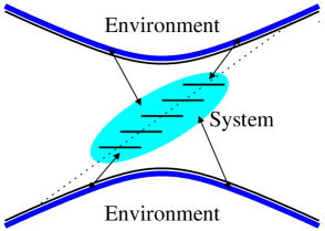
Figure 1: Depiction of the separation between system and bath degrees of freedom. For infinite baths, one cannot construct a local operator of the form Eq. (19), one that is a product of a finite number of terms. If the product is truncated, parity leaks into the bath.

Finally, we would also like to mention that the above scheme, with simple, non-compound, Majorana encoding, generalizes to multiple qubits. One possible encoding (though not the most economical) is to use four vortices and as such four Majorana modes per qubit. For this and any other encoding all possible correlators for the quantum memory may be expressed as expectation values of various products of Majorana operatorskey-89 . All quantum coherences for our qubits may then be computed by studying Majorana mode correlators which we study below.

In carrying out this program, we will analyze two distinct types of environments: the first is when couplings $\Phi(\vec{r})$ change suddenly but remain static thereafter, and the second when the environment changes dynamically. We show that that in the static environment case the tunneling Hamiltonian merely leads to a finite depletion of the Majorana two-time correlations. In this case, much of the information stored in these modes survives for arbitrarily long times.

More generally, for dynamic environments, we obtain an expression for the rate of loss of information stored in the Majorana operators that depends on the spectral density of the noise and of the fermionic bath. We present several examples of noise that can be studied essentially exactly, for instance classical telegraphic noise, as well as both classical and quantum Gaussian fluctuations.

The results in the paper are presented as follows:

• In Section III we present general considerations involving the coherence properties of Majorana modes. We show that under reasonably generic initial conditions the coherence of the Majorana modes does not depend on their initial states. Furthermore we show that the two time correlation functions, coherences, factorize as a product over coherences for individual Majorana modes, that make up the quantum memory, interacting with their individual environments. As such we may reduce the problem of the coherence of the quantum memory to the problem of the coherence of one Majorana mode in tunneling contact with a (gapped) fermionic reservoir.

• In Section IV we take a first step towards a calculation of the coherence of a single Majorana mode. We begin by describing the Keldysh technique relevant to Majorana modes. We present combinatorial tricks that make is possible to efficiently convert Keldysh computations using a mixture of Majorana and regular fermionic modes into a more familiar computation which uses only regular fermion modes. We then present an example where, for simplicity, we treat the fermions in the bath as free (non-relaxing approximation). We also present a general formula for the coherence of a Majorana qubit that is used several times in the remaining analysis.

• In Section V we present several related classical models for the fluctuations of the bath. We solve these models essentially exactly, by mapping the problem of the coherence of a single Majorana mode to the problem of a particle undergoing classical diffusion. We use this technique to study classical fluctuations of the tunneling amplitudes and energy levels of the reservoir (we primarily focus on Gaussian fluctuations). In all cases we find decoherence with a rate that depends on the spectral density of the fluctuations in the reservoir. In many cases the decoherence due to an individual fermion mode has a power law time dependence but it will turn out that a bath made of many weakly interacting modes leads to exponential decay of coherence for intermediate times.

• In Section VI we conclude. In light of the results we obtain in this paper, we critically examine the degree in which quantum memories can be encoded using Majorana fermions when these are in contact with a dynamical environment. We show that the coherence of the Majorana mode is controlled by the coherence of the bath it interacts with.

• In Appendix A we compute exact dressed zero modes for static quadratic Hamiltonians, which we use to verify the validity of our results in Section IV. In Appendix B we present a rather technical calculation of a Majorana mode interacting with a fermionic bath with fully quantum mechanical Gaussian fluctuations. To leading order we find a decay similar to classical computations. In Appendix C we present various technical calculations, used throughout the rest of the text. In particular, in Appendix C.1 we show that our results are independent of coding subspace, in Appendix C.3 we present some technical arguments (which are used in Section V) in favor of weak (negligible) coupling of the fluctuation for the various fermionic modes. In the rest of the appendix we derive formulas used in the main text.

III Dynamics

We begin with a study of the general properties of the dynamics of a system of Majorana modes. We will focus on a computation of correlators involving Majorana operators. This will allow us to study the coherence properties of a topological quantum memory which is based on qubits made up of localized zero energy modes. In this Section we will adhere to very general Hamiltonians and we will study only properties that are essentially independent of the form of this Hamiltonian. This will set us up for studies of specific types of Hamiltonians in Section IV. From the outset, we would like to specify the initial conditions or equivalently the density matrix when the system is initialized at $t=0$. We will assume that initially the density matrix factorizes into a product of the form:

$$\rho_{\mathrm{tot}}=\rho_{\mathrm{Maj}}\otimes\prod_{i}\rho_{\mathrm{env_{i}}}$$ (20)

Here $\rho_{\mathrm{tot}}$ is the density matrix for the entire system, while $\rho_{\mathrm{Maj}}$ represents and arbitrary non-equilibrium density matrix for the Majorana modes. The $\rho_{\mathrm{env_{i}}}$ are arbitrary, not-necessarily equilibrium, density matrices for the environments of the individual Majorana modes. No specific “ensemble” is assumed. This form is a reasonable, consistent assumption for the initial states of system plus bath, particularly so, as many experimental methods of initialization produce such states.

For our qubit memory persistence between times $t_{1}$ and $t_{2}$ is captured by the two-time correlators such as $\left\langle\sigma^{z}\left(t_{1}\right)\sigma^{z}\left(t_{2}\right)\right\rangle$. We note that, because the initial, $t=0$, state breaks time-translation invariance, generically these correlators are functions of both $t_{1}$ and $t_{2}$. Here we shall focus specifically on correlations, like $\left\langle\sigma^{z}\left(0\right)\sigma^{z}\left(\mathrm{T}\right)\right\rangle$, between the state prepared at $t=0$ and the state at a later time time $t=\mathrm{T}$ which characterize the degree to which the information encoded in the qubit at the initial time survives interaction with the bath when it is retrieved at a later time $\mathrm{T}$.

The key results of this section, which are used repeatedly later in the text, may be summarized by saying that even though the factorization form given in Eq. (20) does not survive Hamiltonian evolution the expectation values of various correlators like $\left\langle\sigma^{z}\left(0\right)\sigma^{z}\left(\mathrm{T}\right)\right\rangle$ or equivalently products of Majorana fermions, to be defined precisely in Eqs. (24) and (25) below, do factorize into products of expectation values for individual Majorana modes. This factorization survives for arbitrary times.

III.1 General ideas

We will consider a set of Majorana modes each interacting with its own fermionic environment, see Eq. (20). We will see that there is decoherence even without direct interactions between different Majorana modes or between their respective environments. One can show that, in the limit when the spatial separation between the Majorana modes is large, the case when multiple Majorana modes interact with a common fermionic bath reduces to the case of uncorrelated non-interacting baths (see Appendix C.2). The Hamiltonian pertinent to each mode may be written as:

$$H_{\alpha} = \sum_{i=1}^{N_{\alpha}}\gamma_{\alpha}\left[\left(B_{i,\alpha}^{\phantom{\dagger}}\,c_{i,\alpha}^{\phantom{\dagger}}-c_{i,\alpha}^{\dagger}\,B_{i,\alpha}^{\dagger}\right)\right.$$ (21)

$$+ \left.H_{\alpha}^{\mathrm{bath}}\left(\{c_{i,\alpha}^{\phantom{\dagger}},c_{i,\alpha}^{\dagger},B_{i,\alpha}^{\phantom{\dagger}},B_{i,\alpha}^{\dagger}\}\right)\right]\;.$$

Here $B_{i,\alpha}$ are some bosonic modes and $\alpha=\left\{1,2,...\right\}$ labels the Majorana modes. The total Hamiltonian is given by $H=\sum_{\alpha}H_{\alpha}$. We will be interested in correlators of the form $\left\langle\gamma_{\alpha_{1}}\;\gamma_{\alpha_{2}}\dots\gamma_{\alpha_{k}}\;\gamma_{\alpha_{1}}\left(t_{1}\right)\;\gamma_{\alpha_{2}}\left(t_{2}\right)\dots\gamma_{\alpha_{\mathrm{k}}}\left(t_{k}\right)\right\rangle$. Here all operators are in the Heisenberg picture, and $\gamma_{\alpha}\left(t\right)$ is given by

$$\gamma_{\alpha}(t)=\left(\widetilde{\mathcal{T}}\;e^{i\int_{0}^{t}H_{\alpha}\left(\tau\right)d\tau}\right)\;\;\gamma_{\alpha}\;\;\left(\mathcal{T}\;e^{-i\int_{0}^{t}H_{\alpha}\left(\tau\right)d\tau}\right)\;,$$ (22)

where ${\mathcal{T}}$ and $\widetilde{\mathcal{T}}$ stand for time-ordered and anti-time-ordered products, respectively. Notice that $\gamma_{\alpha}\left(t\right)=\gamma_{\alpha}^{\dagger}\left(t\right)$ at all times.

Now, by Taylor expanding the time-ordered and anti-time-ordered exponentials in Eq. (22), taking various commutators, grouping terms and using the fact that $\gamma_{\alpha}^{2}=1$, we may write that

$$\gamma_{\alpha}\left(t\right)=\gamma_{\alpha}\,\mathcal{B}_{\alpha}\left(t\right)+\mathcal{F}_{\alpha}\left(t\right),$$ (23)

with $\mathcal{B}_{\alpha}\left(t\right)$ and $\mathcal{F}_{\alpha}\left(t\right)$ having no factors of $\gamma_{\alpha}$. Because $\gamma_{\alpha}\left(t\right)$ must be fermionic (this can be seen from the fact that the Hamiltonian and all its powers are bosonic) we may deduce that $\mathcal{B}_{\alpha}\left(t\right)$ and $\mathcal{F}_{\alpha}\left(t\right)$ are, respectively, bosonic and fermionic operators. By the conservation of fermion parity we know that the expectation value of any operator $\left\langle\mathcal{F}_{\alpha}\left(t\right)\right\rangle=0$. Finally, because $\gamma_{\alpha}\left(t\right)$ is Hermitian, it also follows from the properties above that $\mathcal{B}_{\alpha}\left(t\right)$ and $\mathcal{F}_{\alpha}\left(t\right)$ are Hermitian as well.

Now, it follows that

$$\left\langle\gamma_{\alpha}\;\gamma_{\alpha}\left(t\right)\right\rangle = \left\langle\mathcal{B}_{\alpha}\left(t\right)\right\rangle+\left\langle\gamma_{\alpha}\,\mathcal{F}_{\alpha}\left(t\right)\right\rangle$$ (24)

$$= \left\langle\mathcal{B}_{\alpha}\left(t\right)\right\rangle+\left\langle\gamma_{\alpha}\right\rangle\,\left\langle\mathcal{F}_{\alpha}\left(t\right)\right\rangle$$

$$= \left\langle\mathcal{B}_{\alpha}\left(t\right)\right\rangle\;,$$

where we used going from the first to the second line of Eq. (24) that the environments and the Majorana states are initially disentangled so expectation values factorize. Note that this comes about because in the Heisenberg picture the expectation values for operators are taken with respect to the initial state, at $t=0$. For the third line we have used that the expectation value of any fermionic operator $\left\langle\mathcal{F}_{\alpha}\left(t\right)\right\rangle$ should be zero. Note that because $\mathcal{B}_{\alpha}\left(t\right)$ is Hermitian this implies that $\left\langle\gamma_{\alpha}\;\gamma_{\alpha}\left(t\right)\right\rangle\in\mathbb{R}$.

The following factorization formula can be similarly showed:

$$\left\langle\gamma_{\alpha_{1}}\dots\gamma_{\alpha_{\mathrm{k}}}\gamma_{\alpha_{1}}\left(t_{1}\right)\dots\gamma_{\alpha_{\mathrm{k}}}\left(t_{k}\right)\right\rangle = \left(-1\right)^{k\left(k-1\right)/2}\;\;\prod_{j=1}^{k}\left\langle\mathcal{B}_{\alpha_{\mathrm{j}}}\left(t_{j}\right)\right\rangle$$ (25)

$$= \left(-1\right)^{k\left(k-1\right)/2}\;\;\prod_{j=1}^{k}\left\langle\gamma_{\alpha_{j}}\;\gamma_{\alpha_{j}}\left(t_{j}\right)\right\rangle\;,$$

for distinct ${\alpha_{j}}$, $j=1,\dots,k$. To show this expression, one uses Eq. (23) and again that the expectation values are computed with respect to the initial density matrix given in Eq. (20) which has the property that the environments are uncorrelated with each other and with the initial Majorana states. We see that this factorization formula is independent of the initial state of the density matrix of the bath. As such our formalism captures highly non-equilibrium initial conditions.

III.2 Qubit memory correlations

The degree of persistence of memories assembled using Majorana fermions can be quantified by the correlation between the qubit state, encoded as in Eq. (8), at two times $0,\,\mathrm{T}$:

$$\left\langle\sigma^{z}\left(0\right)\sigma^{z}\left(\mathrm{T}\right)\right\rangle = -\left\langle\gamma_{1}\left(0\right)\gamma_{2}\left(0\right)\gamma_{1}\left(\mathrm{T}\right)\gamma_{2}\left(\mathrm{T}\right)\right\rangle$$ (26)

$$= \;\;\;\left\langle\gamma_{1}\left(0\right)\gamma_{1}\left(\mathrm{T}\right)\right\rangle\times\left\langle\gamma_{2}\left(0\right)\gamma_{2}\left(\mathrm{T}\right)\right\rangle.$$

Notice that the factorization implies that, even though the qubit is defined non-locally using two spatially separated Majorana fermions, the decay of the memory is controlled by the product of the two-time correlations of the two separate Majorana modes. In particular, the decoherence rate is independent of the initial state of the quantum memory (that is correlators of the form $\left\langle\gamma_{1}\gamma_{2}\right\rangle$ do not enter the result).

Thus in the case of uncoupled well separated Majorana modes each interacting with its own environment the task of determining the persistence of topological quantum memories based on Majorana fermions is reduced to the calculation of the coherences $\left\langle\gamma_{\alpha}\left(0\right)\gamma_{\alpha}\left(\mathrm{T}\right)\right\rangle$ in the presence of different fermionic environments. We carry out this program henceforth.

IV Keldysh calculation of coherence

We now proceed to describe the technical details associated with studying dynamics. For generality and later use we will study both static and time dependent Hamiltonians. Based on the discussion given in Section III for the purposes of computing coherences it will be sufficient to focus on a single Majorana mode. As such we will drop the subscript $\alpha$, see Eq. (21), henceforth.

IV.1 General Observations

We will convert the computation of the Majorana correlations into a Keldysh calculation carried out using only the bosons and regular complex fermions inside the reservoir. (For a review of standard Keldysh techniques see e.g. key-60, ; key-44, ; key-82, .) We will calculate the following correlator:

$$\left\langle\gamma\left(0\right)\gamma\left(T\right)\right\rangle=\left\langle\gamma\;\left(\widetilde{\mathcal{T}}\;e^{+i\int_{0}^{\mathrm{T}}H\left(\tau\right)\,d\tau}\right)\;\gamma\;\left({\mathcal{T}}\;e^{-i\int_{0}^{\mathrm{T}}H\left(\tau\right)\,d\tau}\right)\right\rangle\;.$$ (27)

Here the expectation value is taken relative to the density matrix $\rho_{0}$ at $\tau=0$ while ${\mathcal{T}}$ and $\widetilde{\mathcal{T}}$ stand for time ordering and time antiordering respectively. To make the computations tractable we will assume that $\rho_{0}=\rho_{\mathrm{therm}}\otimes\rho_{\mathrm{Maj}}$. Here $\rho_{\mathrm{Maj}}$ is any initial density matrix acting on the subspace of the Majorana modes while $\rho_{\mathrm{therm}}$ is the thermal density matrix for the regular fermion modes.

To compute the correlator in Eq. (27), we will use Eq. (21) and work in the interaction picture with respect to the rest of the Hamiltonian ${H}^{\mathrm{bath}}\left(\{{c}_{\mathrm{i}}^{\phantom{\dagger}},{c}_{\mathrm{i}}^{\dagger},{B}_{\mathrm{i}}^{\phantom{\dagger}},{B}_{\mathrm{i}}^{\dagger}\}\right)$. We will expand the ordered exponentials in powers of $H$ and collect and contract all the $\gamma$s to eliminate them. In what follows will show that

$$\left\langle\gamma\left(0\right)\gamma\left(T\right)\right\rangle=\left\langle\left(\widetilde{\mathcal{T}}\;e^{-\int_{0}^{\mathrm{T}}\mathrm{O}\left(\tau\right)\,d\tau}\right)\;\left({\mathcal{T}}\;e^{-\int_{0}^{\mathrm{T}}\mathrm{O}\left(\tau\right)\,\mathrm{d}\tau}\right)\right\rangle\equiv\left\langle{\mathcal{T}_{c}}\;e^{-\sum_{a}\int_{0}^{\mathrm{T}}\mathrm{O}\left(\tau^{a}\right)\mathrm{d}\tau^{a}}\right\rangle\;,$$ (28)

where $\mathrm{O}\left(\tau\right)=\sum_{\mathrm{i=1}}^{\mathrm{N}}\left(B_{i}\left(\tau\right)c_{i}\left(\tau\right)-B_{i}^{\dagger}\left(\tau\right)c_{i}^{\dagger}\left(\tau\right)\right)$, and $\mathcal{T}_{\mathrm{c}}$ stands for the Keldysh ordering that combines the forward and backward propagation, and the index $a\,\mathrm{=\,t,\,b}$ labels the two pieces (forward and backward) of the ordered product. (Notice though that the operator $\mathrm{O}\left(\tau\right)$ in the exponential comes with the same sign in the ${\mathcal{T}}$ and $\widetilde{\mathcal{T}}$ products.)

Figure 2: The Keldysh contour determining the coherence of the Majorana zero mode. We consider $2K$ insertions of our interaction Hamiltonian $\pm i\gamma\sum_{i=1}^{N}\left(B_{i}c_{i}-B_{i}^{\dagger}c_{i}^{\dagger}\right)$ into the Keldysh contour with $\pm$ referring to the forward in time and backwards in time branches. Several interaction insertions are shown by dashed lines. To convert this contour to a “regular” Keldysh calculation we commute the Majorana modes ($\gamma$ terms) including the one at $\tau=\mathrm{T}$ till they are all located at $\tau=0$ as shown. In the text we describe how to compute commutators appropriately.

Below we give the essential arguments needed to derive Eq. (28). To carry out this program, let us introduce a short-hand notation $H=\gamma\sum_{i=1}^{N}\left(B_{i}c_{i}-B_{i}^{\dagger}c_{i}^{\dagger}\right)\equiv\gamma\left(\mathbf{B}\mathbf{c}-\mathbf{B}^{\dagger}\mathbf{c}^{\dagger}\right)$. Now expand Eq. (27) in powers of $H$, and focus on the term with $N_{\mathrm{b}}+N_{\mathrm{t}}$ insertions, with $N_{\mathrm{b}}$ from the expansion of the $\widetilde{\mathcal{T}}$-ordered exponential and $N_{\mathrm{t}}$ from that of the ${\mathcal{T}}$-ordered exponential. By fermion parity conservation and using our assumption that the system-bath initial density matrix is factorized we know that $N_{\mathrm{b}}+N_{\mathrm{t}}=2K$ is even. The insertions of our interaction Hamiltonian are of the form

$$\begin{array}[]{l}\overbrace{\{\gamma\}}^{\tau=0}\underbrace{\left[i\gamma\left(\mathbf{B}\mathbf{c}-\mathbf{B}^{\dagger}\mathbf{c}^{\dagger}\right)(t_{1}^{b})\right]\cdots\left[i\gamma\left(\mathbf{B}\mathbf{c}-\mathbf{B}^{\dagger}\mathbf{c}^{\dagger}\right)(t_{N_{\mathrm{b}}}^{\mathrm{b}})\right]}_{\text{bottom insertions}}\overbrace{\{\gamma\}}^{\tau=\mathrm{T}}\underbrace{\left[-i\gamma\left(\mathbf{B}\mathbf{c}-\mathbf{B}^{\dagger}\mathbf{c}^{\dagger}\right)(t_{1}^{t})\right]\cdots\left[-i\gamma\left(\mathbf{B}\mathbf{c}-\mathbf{B}^{\dagger}\mathbf{c}^{\dagger}\right)(t_{N_{\mathrm{t}}}^{\mathrm{t}})\right]}_{\text{top insertions}}\;.\end{array}$$ (29)

We show in curly brackets $\left\{\gamma\right\}$ the modes at $\tau=\mathrm{T}$ and at $\tau=0$, to help single them out for constructing the argument below. Our strategy to convert this calculation to a “regular” Keldysh calculation will be to move the Majorana modes ($\gamma$ terms), including the $\{\gamma\}$ at $\tau=\mathrm{T}$, by taking appropriate commutators, till they are all at the left hand side, adjacent to the $\{\gamma\}$ inserted at $\tau=0$. We will move along the contour ordering direction (see Fig. 2). We will then use the relation $\gamma^{2K+2}=1$ to eliminate these modes altogether. All that remains is a computation of the commutators. Because of the form of the Hamiltonian, computing commutators is equivalent to computing an overall sign for the term in the expansion. By noting that the Hamiltonian is bosonic we obtain that the overall sign is only due to the anti-commutation of the $\gamma$’s with the $c_{i}$ and $c_{i}^{\dagger}$ inside the $\left(\mathbf{B}\mathbf{c}-\mathbf{B}^{\dagger}\mathbf{c}^{\dagger}\right)$ terms. We shall move each $\gamma$ mode to the very left in two steps: we first move the mode at $\tau=\mathrm{T}$ to the very left towards $\tau=0$; then we move all the remaining modes there as well.

In the first part of the procedure is to obtain the contribution of the Majorana fermion inserted at $\tau=\mathrm{T}$. We note that the number of $-1$ signs it picks up depends on its position along the contour relative to the other modes it picks up one $-1$ sign for very mode it passes so there is an overall sign of $\left(-1\right)^{N_{\mathrm{b}}}$.

Now for the rest working from left to right, the first Majorana mode that needs to be moved picks up no $-1$ signs as it does not pass over a $\left(\mathbf{B}\mathbf{c}-\mathbf{B}^{\dagger}\mathbf{c}^{\dagger}\right)$ term, but the second picks up one $-1$ sign as it passes over one such term. Similarly, the third picks up two $(-1)$ signs, and so forth. Finally the $2K$th Majorana mode (last to be moved, sitting all the way to the right) picks up $2K-1$ factors of $-1$. The product of these factors yields $\left(-1\right)^{K\left(2K-1\right)}=\left(-1\right)^{K}=\left(-i\right)^{N_{\mathrm{t}}+N_{\mathrm{b}}}$.

Thus eliminating the $\gamma$’s in Eq. (29) leads to an overall sign ${(-i)^{N_{\mathrm{b}}+N_{\mathrm{t}}}\times(-1)^{N_{\mathrm{b}}}}$, which then allows us to replace terms of the form Eq. (29) by

$$\begin{array}[]{l}\underbrace{\left[-\left(\mathbf{B}\mathbf{c}-\mathbf{B}^{\dagger}\mathbf{c}^{\dagger}\right)(t_{1}^{\mathrm{b}})\right]\cdots\left[-\left(\mathbf{B}\mathbf{c}-\mathbf{B}^{\dagger}\mathbf{c}^{\dagger}\right)(t_{N_{\mathrm{b}}}^{\mathrm{b}})\right]}_{\text{bottom insertions}}\underbrace{\left[-\left(\mathbf{B}\mathbf{c}-\mathbf{B}^{\dagger}\mathbf{c}^{\dagger}\right)(t_{1}^{\mathrm{t}})\right]\cdots\left[-\left(\mathbf{B}\mathbf{c}-\mathbf{B}^{\dagger}\mathbf{c}^{\dagger}\right)(t_{N_{\mathrm{t}}}^{\mathrm{t}})\right]}_{\text{top insertions}}\;.\end{array}$$ (30)

These are precisely the terms that appear in the series expansion of Eq. (28), and therefore we can continue the calculation utilizing this expression. We should point out that for complex fermions coming from Majorana insertion ${\mathcal{T}}_{c}$ corresponds to literal ordering on the Keldysh contour, without any fermionic minus signs, because the original Hamiltonian was bosonic [this can also be seen step-by-step in going from Eq. (29) to Eq. (30)]. This fact leads to the modified sign for the fermionic ${\mathcal{T}}_{c}$-ordering:

$$\mathcal{T}_{c}\left[c_{i}^{\dagger}\left(t_{1}\right)c_{i}\left(t_{2}\right)\right]\equiv\left\{\begin{array}[]{llll}\theta\left(t_{1}-t_{2}\right)\;c_{i}^{\dagger}\left(t_{1}\right)c_{i}\left(t_{2}\right)+\theta\left(t_{2}-t_{1}\right)\;c_{i}\left(t_{2}\right)c_{i}^{\dagger}\left(t_{1}\right)&,\;t_{1},t_{2}\;\mathrm{on\;top}\\ c_{i}^{\dagger}\left(t_{1}\right)c_{i}\left(t_{2}\right)&,\;t_{1}\;\mathrm{on\;bottom},t_{2}\;\mathrm{on\;top}\\ c_{i}\left(t_{2}\right)c_{i}^{\dagger}\left(t_{1}\right)&,\;t_{1}\;\mathrm{on\;top},t_{2}\;\mathrm{on\;bottom}\\ \theta\left(t_{2}-t_{1}\right)\;c_{i}^{\dagger}\left(t_{1}\right)c_{i}\left(t_{2}\right)+\theta\left(t_{1}-t_{2}\right)\;c_{i}\left(t_{2}\right)c_{i}^{\dagger}\left(t_{1}\right)&,\;t_{1},t_{2}\;\mathrm{on\;bottom}\;.\end{array}\right.$$ (31)

Now, we turn our attention to the computation of Eq. (28). We do so in steps, computing the expectation values by first tracing the fermions ($c_{i}\,,\,c_{i}^{\dagger}$) and then subsequently tracing the bosonic degrees of freedom. Even in the case where there are interactions for the fermions, we can still treat the theory as quadratic in the fermions and include the interactions (with photons or phonons) as a coupling of the fermionic bilinears with the mediating bosons, which we label by $\phi$. Alternatively, we may think of the fields $\phi$ fields as Hubbard-Stratonovich decoupling fieldskey-78 .

We can thus write

$$\left\langle{\mathcal{T}_{\mathrm{c}}}\;e^{-\sum_{a}\int_{0}^{\mathrm{T}}\left(\mathbf{B}\mathbf{c}-\mathbf{B}^{\dagger}\mathbf{c}^{\dagger}\right)\left(\tau^{a}\right)\;\mathrm{d}\tau^{a}}\right\rangle={\mathcal{Z}}^{-1}\;\int\left(\prod_{a}\mathcal{D}\mathbf{B}_{a}\,\mathcal{D}\mathbf{B}_{a}^{\dagger}\right)\;e^{i{\mathcal{S}}_{\mathbf{B}}[\mathbf{B}_{a}\,\mathbf{B}_{a}^{\dagger}]}\;\int\left(\prod_{a}\mathcal{D}\mathbf{\phi}_{a}\,\mathcal{D}\mathbf{\phi}_{a}^{\dagger}\right)\;e^{i{\mathcal{S}}_{\mathbf{\phi}}[\mathbf{\phi}_{a}\,\mathbf{\phi}_{a}^{\dagger}]}$$

$$\qquad\qquad\qquad\qquad\qquad\times\;\exp\left(\frac{1}{2}\,{\sum_{a,b}\;\int_{0}^{\mathrm{T}}\!\!\mathrm{d}\tau_{1}^{a}\int_{0}^{\mathrm{T}}\!\!\mathrm{d}\tau_{2}^{b}\;\;\left\langle{\mathcal{T}_{c}}\left[\left(\mathbf{B}\mathbf{c}-\mathbf{B}^{\dagger}\mathbf{c}^{\dagger}\right)\left(\tau_{1}^{a}\right)\;\left(\mathbf{B}\mathbf{c}-\mathbf{B}^{\dagger}\mathbf{c}^{\dagger}\right)\left(\tau_{2}^{b}\right)\right]\right\rangle_{\mathbf{c},\mathbf{c}^{\dagger}}}\right)\;.$$ (32)

We remind the reader that all functional integrals are along the Keldysh contour. The action ${\mathcal{S}}_{\mathbf{\phi}}$ is that of the interaction mediator field $\phi$ and contains the dressing from the integration of the fermions, which are integrated out first as explained above. The normalization ${\mathcal{Z}}$ is

$${\mathcal{Z}}=\int\left(\prod_{a}\mathcal{D}\mathbf{B}_{a}\,\mathcal{D}\mathbf{B}_{a}^{\dagger}\right)\;e^{i{\mathcal{S}}_{\mathbf{B}}[\mathbf{B}_{a}\,\mathbf{B}_{a}^{\dagger}]}\;\int\left(\prod_{a}\mathcal{D}\mathbf{\phi}_{a}\,\mathcal{D}\mathbf{\phi}_{a}^{\dagger}\right)\;e^{i{\mathcal{S}}_{\mathbf{\phi}}[\mathbf{\phi}_{a}\,\mathbf{\phi}_{a}^{\dagger}]}\;.$$ (33)

This procedure works because it possible to calculate partition functions, Green’s functions, integrate fields out etc. along any contour, in particular along the Keldysh contour as used here. We then express the fermionic correlators in terms of their Green’s function,

$$\left\langle{\mathcal{T}_{\mathrm{c}}}\left[\left(\mathbf{B}\mathbf{c}-\mathbf{B}^{\dagger}\mathbf{c}^{\dagger}\right)\left(\tau_{1}^{a}\right)\;\left(\mathbf{B}\mathbf{c}-\mathbf{B}^{\dagger}\mathbf{c}^{\dagger}\right)\left(\tau_{2}^{b}\right)\right]\right\rangle_{\mathbf{c},\mathbf{c}^{\dagger}} = -{B_{i}}\left(\tau_{1}^{a}\right){B_{j}}^{\dagger}\left(\tau_{2}^{b}\right)\;\left\langle{\mathcal{T}_{\mathrm{c}}}\left[{c_{i}}\left(\tau_{1}^{a}\right)\;{c_{j}}^{\dagger}\left(\tau_{2}^{b}\right)\right]\right\rangle$$ (34)

$$-\;{B_{i}}^{\dagger}\left(\tau_{1}^{a}\right){B_{j}}\left(\tau_{2}^{b}\right)\;\left\langle{\mathcal{T}_{\mathrm{c}}}\left[{c_{i}}^{\dagger}\left(\tau_{1}^{a}\right)\;{c_{j}}\left(\tau_{2}^{b}\right)\right]\right\rangle$$

$$\equiv -\mathbf{B}\left(\tau_{1}^{a}\right)\;G_{\mathrm{F,e}}^{\phi}\left(\tau_{1}^{a},\tau_{2}^{b}\right)\;\mathbf{B}^{\dagger}\left(\tau_{2}^{b}\right)$$

$$-\;\mathbf{B}^{\dagger}\left(\tau_{1}^{a}\right)\;G_{\mathrm{F,h}}^{\phi}\left(\tau_{1}^{a},\tau_{2}^{b}\right)\;\mathbf{B}\left(\tau_{2}^{b}\right),$$

where the $G_{\mathrm{F,e}}^{\phi}\left(\tau_{1}^{a},\tau_{2}^{b}\right)$ and $G_{\mathrm{F,h}}^{\phi}\left(\tau_{1}^{a},\tau_{2}^{b}\right)$ are, respectively, the electron and hole fermionic Green’s function, and we have used the fact that the bosonic fields $\mathbf{B}\,,\,\mathbf{B}^{\dagger}$ can be treated as c-numbers as they are inside the bosonic path integral. As stated previously $G_{\mathrm{F,e}}^{\phi}\left(\tau_{1}^{a},\tau_{2}^{b}\right)$ and $G_{\mathrm{F,h}}^{\phi}\left(\tau_{1}^{a},\tau_{2}^{b}\right)$ are slightly unusual Green’s functions, with no fermionic minus signs (only plus signs), as shown in Eq. (31). Let us define $D_{\mathrm{F}}^{\phi}\left(\tau_{1}^{a},\tau_{2}^{b}\right)=\;G_{\mathrm{F,h}}^{\phi}\left(\tau_{1}^{a},\tau_{2}^{b}\right)+\;G_{\mathrm{F,e}}^{\phi}\left(\tau_{2}^{b},\tau_{1}^{a}\right)$, so we can then write

$$\left\langle\gamma\left(0\right)\gamma\left(T\right)\right\rangle={\mathcal{Z}}^{-1}\;\int\left(\prod_{a}\mathcal{D}\mathbf{B}_{a}\,\mathcal{D}\mathbf{B}_{a}^{\dagger}\right)\;e^{i{\mathcal{S}}_{\mathbf{B}}[\mathbf{B}_{a}\,\mathbf{B}_{a}^{\dagger}]}\;\int\left(\prod_{a}\mathcal{D}\mathbf{\phi}_{a}\,\mathcal{D}\mathbf{\phi}_{a}^{\dagger}\right)\;e^{i{\mathcal{S}}[\mathbf{\phi}_{a}\,\mathbf{\phi}_{a}^{\dagger}]}$$

$$\qquad\qquad\qquad\times\;\exp\left(-\frac{1}{2}\,{\sum_{a,b}\;\int_{0}^{\mathrm{T}}\!\!\mathrm{d}\tau_{1}^{a}\int_{0}^{\mathrm{T}}\!\!\mathrm{d}\tau_{2}^{b}\;\;\mathbf{B}^{\dagger}\left(\tau_{1}^{a}\right)\;D_{\mathrm{F}}^{\phi}\left(\tau_{1}^{a},\tau_{2}^{b}\right)\;\mathbf{B}\left(\tau_{2}^{b}\right)}\right)\;.$$ (35)

We remark that the expression in Eq. (35) was derived without any approximations. It holds for interacting electrons as well, as long as the interactions are included via an external bosonic field denoted by $\phi$ above. Furthermore we would like to note that though it is not used anywhere in this paper, but a similar path integral formulation using Grassmann variables may be done without any decoupling fields, for regular quartic $\sim\Psi^{\dagger}\left(\vec{x}\right)\Psi^{\dagger}\left(\vec{x}\right)\Psi\left(\vec{x}\right)\Psi\left(\vec{x}\right)$ fermionic interactions. A systematic Keldysh diagrammatic perturbation theory may be derived from it.

For future use we note that to compute the coherence of a Majorana mode it is often enough to compute the four diagrams shown in Fig. (3). Following Eq. (35), their sum may be explicitly written as:

$$V\left(T\right) \equiv \sum_{a,b}\;\int_{0}^{\mathrm{T}}\!\!\mathrm{d}\tau_{1}^{a}\int_{0}^{\mathrm{T}}\!\!\mathrm{d}\tau_{2}^{b}\;\;\mathbf{B}^{\dagger}\left(\tau_{1}^{a}\right)\;D_{\mathrm{F}}^{\phi}\left(\tau_{1}^{a},\tau_{2}^{b}\right)\;\mathbf{B}\left(\tau_{2}^{b}\right)$$

$$= 2\sum_{i}\left\{\int_{0}^{\mathrm{T}}d\tau_{1}\int_{0}^{\mathrm{T}}d\tau_{2}\left[\mathcal{T}\left({B_{i}}^{\dagger}\left(\tau_{1}^{\mathrm{t}}\right){B_{i}}\left(\tau_{2}^{\mathrm{\mathrm{t}}}\right)\right)\times\left(\theta\left(\tau_{1}-\tau_{2}\right)\left\langle c_{i}^{\dagger}\left(\tau_{1}\right)c_{i}\left(\tau_{2}\right)\right\rangle+\theta\left(\tau_{2}-\tau_{1}\right)\left\langle c_{i}\left(\tau_{2}\right)c_{i}^{\dagger}\left(\tau_{1}\right)\right\rangle\right)\right.\right.$$

$$+ \widetilde{\mathcal{T}}\left({B_{i}}^{\dagger}\left(\tau_{1}^{\mathrm{b}}\right){B_{i}}\left(\tau_{2}^{\mathrm{\mathrm{b}}}\right)\right)\times\left(\theta\left(\tau_{2}-\tau_{1}\right)\left\langle c_{i}^{\dagger}\left(\tau_{1}\right)c_{i}\left(\tau_{2}\right)\right\rangle+\theta\left(\tau_{1}-\tau_{2}\right)\left\langle c_{i}\left(\tau_{2}\right)c_{i}^{\dagger}\left(\tau_{1}\right)\right\rangle\right)$$

$$+ \left.\left.\left({B_{i}}^{\dagger}\left(\tau_{1}^{\mathrm{t}}\right){B_{i}}\left(\tau_{2}^{\mathrm{\mathrm{b}}}\right)\left\langle c_{i}^{\dagger}\left(\tau_{1}\right)c_{i}\left(\tau_{2}\right)\right\rangle+{B_{i}}\left(\tau_{1}^{\mathrm{t}}\right){B_{i}^{\dagger}}\left(\tau_{2}^{\mathrm{\mathrm{b}}}\right)\left\langle c_{i}\left(\tau_{1}\right)c_{i}^{\dagger}\left(\tau_{2}\right)\right\rangle\right)\right]\right\}$$

Here $\mathcal{T}$, $\widetilde{\mathcal{T}}$ refer to time ordering and time anti-ordering operators. This form places the time ordering or antiordering terms ($\mathcal{T}\left({B_{i}}^{\dagger}\left(\tau_{1}^{\mathrm{t}}\right){B_{i}}\left(\tau_{2}^{\mathrm{\mathrm{t}}}\right)\right)$) with the appropriate fermion correlators so it can be used directly in calculations without having to use a path integral. The factor of two going from the first to the second line comes from a symmetry $\tau_{1}\leftrightarrow\tau_{2}$ (which also allowed us to simplify Eq. (IV.1) above to contain six rather then twelve terms). Because of exponentiation of disconnected diagrams, if we can safely ignore higher order correlations among the ${B_{i}}$’s, we may write that:

$$\left\langle\gamma\left(0\right)\gamma\left(T\right)\right\rangle=\mathrm{e}^{-\frac{1}{2}\left\langle V\left(T\right)\right\rangle}\;.$$ (37)

A quick way to derive the extra factor of $\frac{1}{2}$ in Eq. (37) above is by noting that it is a symmetry factor associated with the ability to permute the two Majorana insertions without changing the diagram [alternatively we can do a combinatorial check, or use Eq. (35)].

Let us illustrate with a few simple examples how one can use the expression for the Majorana correlations $\left\langle\gamma\left(0\right)\gamma\left(T\right)\right\rangle$ in Eq. (35) to calculate the the decay rates of topological memories. We then deploy this expression in detailed studies for fluctuating Hamiltonians in Section V.

Figure 3: The four diagrams relevant to calculating $V\left(T\right)$ in the main text. We need to sum over four possible orderings of the Majorana insertions on the Keldysh contour. The value is given by a sum of terms like ${B_{i}}^{\dagger}\left(\tau_{1}^{\mathrm{t}}\right){B_{i}}\left(\tau_{2}^{\mathrm{\mathrm{b}}}\right)\left\langle c_{i}^{\dagger}\left(\tau_{1}\right)c_{i}\left(\tau_{2}\right)\right\rangle$.

IV.2 Simple examples

Let us consider simple cases where the $B_{i}$ are simply constants $\Gamma_{i}$, switched on at $\tau=0$. In this case the expression in Eq. (35) simplifies to

$$\left\langle\gamma\left(0\right)\gamma\left(T\right)\right\rangle={\mathcal{Z}}^{-1}\;\;\int\left(\prod_{a}\mathcal{D}\mathbf{\phi}_{a}\,\mathcal{D}\mathbf{\phi}_{a}^{\dagger}\right)\;e^{i{\mathcal{S}}[\mathbf{\phi}_{a}\,\mathbf{\phi}_{a}^{\dagger}]}$$

$$\qquad\qquad\qquad\times\;\exp\left(-\frac{1}{2}\,{\sum_{a,b}\;\int_{0}^{\mathrm{T}}\!\!\mathrm{d}\tau_{1}^{a}\int_{0}^{\mathrm{T}}\!\!\mathrm{d}\tau_{2}^{b}\;\;\mathbf{\Gamma}^{\dagger}\;D_{\mathrm{F}}^{\phi}\left(\tau_{1}^{a},\tau_{2}^{b}\right)\;\mathbf{\Gamma}}\right)$$

$$\qquad\qquad\qquad=\exp\left(-\frac{1}{2}\,{\sum_{a,b}\;\int_{0}^{\mathrm{T}}\!\!\mathrm{d}\tau_{1}^{a}\int_{0}^{\mathrm{T}}\!\!\mathrm{d}\tau_{2}^{b}\;\;\mathbf{\Gamma}^{\dagger}\;\overline{D}_{F}^{(2)}\left(\tau_{1}^{a},\tau_{2}^{b}\right)\;\mathbf{\Gamma}}\;+\;\dots\right)\;,$$ (38)

where $\overline{\mathrm{D}}_{\mathrm{F}}^{(2)}\left(\tau_{1}^{a},\tau_{2}^{b}\right)=\;\overline{\mathrm{G}}_{\mathrm{F,h}}^{(2)}\left(\tau_{1}^{a},\tau_{2}^{b}\right)+\;\overline{\mathrm{G}}_{\mathrm{F,e}}^{(2)}\left(\tau_{2}^{b},\tau_{1}^{a}\right)$, with $\overline{\mathrm{G}}_{\mathrm{F,h}}^{(2)}$ and $\overline{\mathrm{G}}_{\mathrm{F,e}}^{(2)}$ exact 2-point electron and hole Keldysh propagators, including the effects of interactions. To be explicit at this level of approximation our formalism handles all the dynamics of the $\phi_{a}$ fields but treats fermionic interactions to quadratic order. The $\dots$ stand for terms of order ${\mathcal{O}}(\mathbf{\Gamma}^{4})$ that involve the 4-point Green’s functions $\overline{\mathrm{G}}^{(4)}$. We shall not do so in this paper, but by including these ${\mathcal{O}}(\mathbf{\Gamma}^{4})$ and higher terms it is possible to handle all fermionic interactions as well.

Taking into account all the four cases in the sum over top and bottom insertions $\sum_{a,b}$, one can write

$$\frac{1}{2}\,{\sum_{a,b}\;\int_{0}^{\mathrm{T}}\!\!\!\!\mathrm{d}\tau_{1}^{a}\int_{0}^{\mathrm{T}}\!\!\!\!\mathrm{d}\tau_{2}^{b}\;\;\mathbf{\Gamma}^{\dagger}\;\overline{\mathrm{D}}_{\mathrm{F}}^{(2)}\left(\tau_{1}^{a},\tau_{2}^{b}\right)\;\mathbf{\Gamma}}=\sum_{i,j}\!\!\int_{0}^{\mathrm{T}}\!\!\!\!\mathrm{d}\tau_{1}\int_{0}^{\mathrm{T}}\!\!\!\!\mathrm{d}\tau_{2}\;\;\Gamma_{i}^{*}\left(\langle\{c_{i}^{\dagger}(\tau_{1}),c_{j}(\tau_{2})\}\rangle\right)\Gamma_{j}\;.$$ (39)

We now consider a case where this formula will be particularly useful. We Consider the case when the bath is described by the Hamiltonian

$$H=\gamma\sum_{i=1}^{N}\left(\Gamma_{i}c_{i}-\Gamma_{i}^{*}c_{i}^{\dagger}\right)+\sum_{i=1}^{N}\epsilon_{i}c_{i}^{\dagger}c_{i}\;.$$ (40)

In this case we have

$$\langle\{c_{i}^{\dagger}(\tau_{1}),c_{j}(\tau_{2})\}\rangle=\delta_{ij}\;e^{-i\epsilon_{\mathrm{i}}(\tau_{1}-\tau_{2})}$$ (41)

with $\epsilon_{i}$ the energy of mode $i$. It follows by substitution in Eq. (39) and then in Eq. (35) that

$$\left\langle\gamma\left(0\right)\gamma\left(\mathrm{T}\right)\right\rangle=\mathrm{e}^{-2\sum_{i}|\Gamma_{i}|^{2}|\int_{0}^{\mathrm{T}}d\tau\;e^{-i\mathrm{\epsilon}_{i}\tau}|^{2}}\;,$$ (42)

or

$$\left\langle\gamma\left(0\right)\gamma\left(\mathrm{T}\right)\right\rangle=\mathrm{e}^{-4\sum_{i}\frac{|\Gamma_{i}|^{2}}{\epsilon_{i}^{2}}[1-\cos(\epsilon_{i}T)]}\;.$$ (43)

If the bath has energy eigenenergies $\epsilon_{i}$ away from zero energy (i.e., there is a gap $\tilde{\epsilon}<|\epsilon_{i}|$), we may drop the oscillating terms in the limit of $\mathrm{T}\gg 1/\tilde{\epsilon}$, so we can write

$$\left\langle\gamma\left(0\right)\gamma\left(\mathrm{T}\right)\right\rangle\approx e^{-4\sum_{i}\frac{|\Gamma_{i}|^{2}}{\epsilon_{i}^{2}}}\;,\quad\mathrm{T}\gg 1/\tilde{\epsilon}\;.$$ (44)

In this case, the Majorana memory decays to $\mathrm{T}$ independent plateaus at large times. Thus, as long as the sum $\sum\frac{|\Gamma_{i}|^{2}}{\epsilon_{i}^{2}}$ converges, the memory is retained to a finite extent. This result is confirmed by a time-independent re-diagonalization in the presence of the $\Gamma_{i}$, which is shown explicitly in Appendix A where a new exact zero mode is calculated. Here we simply note that the finite depletion found in this case is a simple consequence of the fact that the modes change once the coupling is switched on. Also, we compute the sum $\sum\frac{|\Gamma_{i}|^{2}}{\epsilon_{i}^{2}}$, and find it to be finite, for a specific tunneling model in Appendix C.4.4.

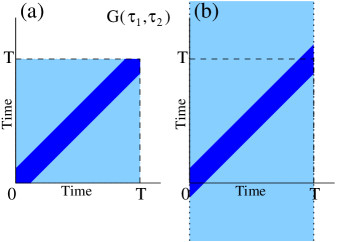
Figure 4: The two time correlators of the tunneling amplitude $G_{\Gamma}\left(\tau_{1},\tau_{2}\right)=\left\langle\Gamma^{*}\left(\tau_{1}\right)\Gamma\left(\tau_{2}\right)\right\rangle$. a) The shaded region represents the actual area of integration for Eq. (52). The darker stripe represents the area of large values for the correlator. This represents strong correlations in the tunneling amplitudes. From this we see that the majority of the integrals appearing in Eq. (52) come from times when $\tau_{\mathrm{1}}\cong\tau_{2}$. b) A simplified integration area. The darkly shaded area of large correlators does not change significantly. As such geometrically we see that this should not change the values of the various correlation functions we are studying. From this it is particularly easy to derive the estimates used in Eq. (55), in particular the linear in $\mathrm{T}$ scaling can now be derived by simply changing co-ordinates in the integral in Eq. (52).

V Fluctuating Hamiltonians

So far we have studied static Hamiltonians. To gain further insight it is interesting to extend our results to fluctuating couplings (which may come from time dependent classical fluctuations or from quantum dynamics). We shall focus on three cases, in all three the fermionic action is quadratic. In the first case we study we consider the situation when the $B_{i}$ are simply replaced by classical variables $\Gamma_{i}$, like we did in Sec. IV.2, but now they depend on time. The second case is that when the energies $\epsilon_{i}$ of the electrons in the bath fluctuate in time, because of environmental fluctuations. The third case is a generalization of the first one, where we treat the $B_{i}$ quantum mechanically with their fluctuations governed by a quadratic action. We treat the first two cases here, and the third, more technical one, in Appendix B.

In the first two cases, one can generalize the expression in Eq. (42) simply by taking $\Gamma_{i}\to\Gamma_{i}(\tau)$ or $\epsilon_{i}\to\epsilon_{i}(\tau)$:

$$\left\langle\gamma\left(0\right)\gamma\left(T\right)\right\rangle = \mathrm{e}^{{-2\sum_{i}\left|\int_{0}^{\mathrm{T}}d\tau\;\Gamma_{i}(\tau)\;e^{-i\int_{0}^{\tau}dt\,\epsilon_{i}(t)}\right|^{2}}}$$ (45)

$$= \prod_{i}\mathrm{e}^{-2\left|\int_{0}^{\mathrm{T}}\mathrm{d}\tau\;\Gamma_{i}(\tau)\;e^{-i\int_{0}^{\tau}dt\,\epsilon_{i}(t)}\right|^{2}}\,,$$

and then average over statistical fluctuations of the $\Gamma_{i}(\tau)$ and $\epsilon_{i}(\tau)$.

The computation of the Majorana correlations can be greatly simplified as follows. Notice that, for each mode $i$, the argument in the exponential in Eq. (45) can be viewed as the magnitude square of the position $\vec{Z}_{i}$ of a particle moving in two-dimensions, or alternatively the modulus square of a complex number $\mathrm{Z}_{i}$ moving on the plane:

$$Z_{i}(\mathrm{T})=\sqrt{2}\int_{0}^{\mathrm{T}}d\tau\;\Gamma_{i}(\tau)\;\mathrm{e}^{-\mathrm{i}\int_{0}^{\tau}dt\,\epsilon_{i}\left(t\right)}\;,$$ (46)

with

$$\left\langle\gamma\left(0\right)\gamma\left(T\right)\right\rangle=\prod_{\mathrm{i}}\mathrm{e}^{-|\vec{Z}_{i}|^{2}}\;.$$ (47)

Below we will argue both in the cases of fluctuating amplitudes $\Gamma_{i}(\tau)$ and energies $\epsilon_{i}(\tau)$ that the probability distribution for the “position” $\vec{Z}_{i}$ is Gaussian:

$$\mathrm{P}(\vec{{Z}}_{i})=\frac{1}{2\pi\sigma_{i}^{2}(\mathrm{T})}\;\exp\left(-\frac{1}{2}\frac{|\vec{Z}_{i}|^{2}}{\sigma_{i}^{2}(\mathrm{T})}\right)\;,$$ (48)

with $\sigma_{i}(\mathrm{T})$ the time-dependent width of the distribution, which we will compute below for each case. With this Gaussian distribution for the $\vec{Z}_{i}$, we can compute the average Majorana correlation,

$$\overline{\left\langle\gamma\left(0\right)\gamma\left(\mathrm{T}\right)\right\rangle} = \prod_{i}\int d^{2}Z_{i}\;P(\vec{Z}_{i})\;e^{-|\vec{Z}_{i}|^{2}}$$ (49)

$$= \prod_{i}\left[1+2\,\sigma_{i}^{2}(\mathrm{T})\right]^{-1}$$

$$\approx \exp\left[-2\,\sum_{i}\sigma_{i}^{2}(\mathrm{T})\right]\;.$$

In the last step we assumed that there are many modes in the fermionic bath, each making a small contribution (or order inverse volume) so we may re-exponentiate the product. The examples below are studied using this expression.

V.1 Fluctuating amplitudes

The fluctuations of the $\Gamma_{i}$ are assumed to be Gaussian distributed according to

$$\mathrm{P}\left(\{\Gamma_{\mathrm{i}}(\tau),\Gamma_{\mathrm{i}}^{*}(\tau)\}\right)={\mathcal{N}}^{-1}\;e^{-\frac{1}{2}\int_{-\infty}^{\infty}d\tau_{1}\int_{-\infty}^{\infty}d\tau_{2}\;\Gamma_{\mathrm{i}}^{*}(\tau_{1})\;G_{\Gamma_{i}}^{-1}(\tau_{1},\tau_{2})\;\Gamma_{\mathrm{i}}(\tau_{2})}\;.$$ (50)

Let us show that the distribution of the $\mathrm{P}(\vec{Z}_{i})$ is Gaussian, and relate $\sigma_{i}(\mathrm{T})$ to the fluctuations of the $\Gamma_{i}$. That the distribution $\mathrm{P}(\vec{Z}_{i})$ should be Gaussian is not surprising since at long times the particle is diffusing. We can write for the characteristic function distribution (Fourier transform of the probability distribution $\mathrm{P}(\vec{Z}_{i})$);

$$\tilde{P}\left(\vec{k}\right) = \int d^{2}\vec{\mathrm{Z}}_{i}\;P(\vec{\mathrm{Z}}_{i})\;e^{-i\vec{k}\cdot\vec{Z}_{i}}$$ (51)

$$= {\mathcal{N}}^{-1}\int\mathcal{D}\Gamma_{i}\,\mathcal{D}\Gamma_{i}^{*}\;\;\mathrm{e}^{-\frac{1}{2}\int_{-\infty}^{\infty}d\tau_{1}\int_{-\infty}^{\infty}d\tau_{2}\;\Gamma_{i}^{*}(\tau_{1})\;G_{\Gamma_{i}}^{-1}(\tau_{1},\tau_{2})\;\Gamma_{i}(\tau_{2})}$$

$$\qquad\qquad\qquad\times e^{-i\frac{1}{2}\,k^{*}\sqrt{2}\int_{0}^{\mathrm{T}}d\tau\;\Gamma_{i}(\tau)\;e^{-i\epsilon_{i}\tau}}\;\times e^{-i\frac{1}{2}\,k\sqrt{2}\int_{0}^{\mathrm{T}}d\tau\;\Gamma_{i}^{*}(\tau)\;e^{+i\epsilon_{i}\tau}}$$

$$= \exp\left(-\frac{1}{2}\,|k|^{2}\times 2\times\int_{0}^{\mathrm{T}}\!\!\!\!d\tau_{1}\;\int_{0}^{\mathrm{T}}\!\!\!\!d\tau_{2}\;\;e^{-i\epsilon_{i}\tau_{1}}\;G_{\Gamma_{i}}(\tau_{1},\tau_{2})\;e^{+i\epsilon_{i}\tau_{2}}\right)\;.$$

Therefore, the distribution $P\left(\vec{Z_{i}}\right)$ is Gaussian, with a variance given by

$$\sigma_{i}^{2}(\mathrm{T})=2\int_{0}^{\mathrm{T}}\!\!\!\!d\tau_{1}\;\int_{0}^{\mathrm{T}}\!\!\!\!d\tau_{2}\;\;e^{-i\epsilon_{i}\tau_{1}}\;G_{\Gamma_{i}}(\tau_{1},\tau_{2})\;e^{+i\epsilon_{i}\tau_{2}}\;.$$ (52)

If the noise correlations are invariant under time-translation, then $G_{\Gamma_{i}}(\tau_{1},\tau_{2})=G_{\Gamma_{i}}(\tau_{1}-\tau_{2})$. We can expand these correlations in frequency domain, $G_{\Gamma_{i}}(\tau_{1}-\tau_{2})=\int_{-\infty}^{\infty}d\omega\;\tilde{G}_{\Gamma_{i}}(\omega)\;e^{-i\omega(\tau_{1}-\tau_{2})}$.

We proceed to compute $\sigma_{i}^{2}(\mathrm{T})$ in Eq. (52) for two distinct cases of low and of high frequency noise.

Case I: Low-frequency noise

In this case, we shall assume that all frequencies $\omega$ for which $\tilde{G}_{\Gamma_{i}}(\omega)$ has significant weight fall below the fermionic energies $\epsilon_{i}$. It the follows that

$$\sigma_{i}^{2}(\mathrm{T}) = 2\int_{|\omega|\ll\tilde{\epsilon}}\!\!\!\!\!\!d\omega\;\sum_{i}\frac{1-\cos[(\epsilon_{i}+\omega)T]}{(\epsilon_{i}+\omega)^{2}}\;\tilde{G}_{\Gamma_{i}}(\omega)\;$$ (53)

$$\approx 2\sum_{i}\frac{1}{\epsilon_{i}^{2}}\;\int_{|\omega|\ll\tilde{\epsilon}}\!\!\!\!\!\!d\omega\;\tilde{G}_{\Gamma_{i}}(\omega)\;.$$

We thus arrive at a correlation decay, for the Majorana modes, of the form

$$\overline{\left\langle\gamma\left(0\right)\gamma\left(\mathrm{T}\right)\right\rangle} \approx \exp\left[-4\sum_{i}\frac{1}{\epsilon_{i}^{2}}\int_{|\omega|\ll\tilde{\epsilon}}\!\!\!\!\!\!d\omega\;\tilde{G}_{\Gamma_{i}}(\omega)\;\right]\;.$$ (54)

The coefficient in the exponent depends on the spectral weight of the noise. From Parceval’s theorem, $\int_{-\infty}^{\infty}d\omega\;\tilde{G}_{\Gamma_{i}}(\omega)=\overline{|\Gamma_{i}(t)|^{2}}$, so the prefactor depends on the intensity of fluctuations of the couplings $\Gamma_{i}(t)$ in time. When the fluctuations are large, for example when the $\Gamma_{i}(t)$ are tied to thermally induced vibrations in two dimensional systems, there is large decoherence.

We remark that even in the cases when $\sigma_{i}^{2}(\mathrm{T}\to\infty)$ is bounded, the value may be rather large, and the Majorana correlation is exponential in this value. Therefore keeping the error to within reasonable bounds for quantum error correction to be applicable can be a tall order. In this sense, the Majorana qubit is not necessarily any more robust than other proposed qubit platforms.

Case II: High-frequency noise

In this case we compute $\sigma_{i}^{2}(\mathrm{T})$ assuming that the correlations $G_{\Gamma_{i}}(\tau_{1}-\tau_{2})$ decay in time, so one can break the $\tau_{1,2}$ integrals into center of mass: $(\tau_{1}+\tau_{2})/2$ and relative coordinates $\tau_{1}-\tau_{2}$ integrals, and in the limit of large $\mathrm{T}$ one has

$$\sigma_{i}^{2}(\mathrm{T})\xrightarrow[\mathrm{T\;large}]{}2\mathrm{T}\;\tilde{G}_{\Gamma}(\epsilon_{i})\;,$$ (55)

where $\tilde{G}_{\Gamma}(\epsilon_{i})$ is the Fourier transform of $\mathrm{G_{\Gamma}(\tau)}$ at frequency $\epsilon_{i}$. We further clarify this in Fig. (4).

We thus arrive at a correlation decay, for the Majorana modes, of the form

$$\overline{\left\langle\gamma\left(0\right)\gamma\left(\mathrm{T}\right)\right\rangle} \approx \exp\left[-4\,\mathrm{T}\sum_{i}\tilde{G}_{\Gamma}(\epsilon_{i})\right]\;.$$ (56)

Notice that this expression has meaning only if the $\tilde{G}_{\Gamma}(\omega)$ has spectral weight above the gap $\tilde{\epsilon}$. If not, one has to treat the problem in the low frequency limit discussed above.

V.1.1 Non zero expectation values

One can generalize this result for when the $\Gamma_{i}$ fluctuations are centered around a non-zero value $\Gamma_{i}^{0}$. In this case,

$$P(\vec{Z}_{i})=\frac{1}{2\pi\sigma_{i}^{2}(\mathrm{T})}\;\exp\left(-\frac{1}{2}\frac{|\vec{Z}_{i}-\vec{Z}_{i}^{0}(\mathrm{T})|^{2}}{\sigma_{i}^{2}(\mathrm{T})}\right)\;\;,$$ (57)

where

$$Z_{i}^{0}(\mathrm{T})=\sqrt{2}\Gamma_{i}^{0}\;\int_{0}^{\mathrm{T}}d\tau\;e^{-i\epsilon_{i}\tau}=\sqrt{2}i\,\Gamma_{i}^{0}\;\frac{e^{-i\epsilon_{i}\mathrm{T}}-1}{\epsilon_{i}}\;\;,$$ (58)

which lead to

$$\mathrm{\overline{\left\langle\gamma\left(0\right)\gamma\left(\mathrm{T}\right)\right\rangle}} = \prod_{i}\frac{e^{-\frac{|Z_{i}^{0}(\mathrm{T})|^{2}}{1+2\sigma_{i}({\mathrm{T}})}}}{1+2\sigma_{i}({\mathrm{T}})}\;.$$ (59)

Notice that we recover the static result Eq. (43) of the previous section if there is no disorder [$\sigma_{i}({\mathrm{T}})=0$]. Indeed we see that $\left\langle\gamma\left(0\right)\gamma\left(\mathrm{T}\right)\right\rangle=\prod_{i}e^{-|Z_{i}^{0}(\mathrm{T})|^{2}}$.

In the particular case of high-frequency noise (non-zero $G_{\Gamma_{i}}(\epsilon_{i})$), one obtains in the large $\mathrm{T}$ limit one obtains

$$\mathrm{\overline{\left\langle\gamma\left(0\right)\gamma\left(\mathrm{T}\right)\right\rangle}}\xrightarrow[\mathrm{T\;large}]{}\prod_{i}\left[1+4T\widetilde{G}_{\Gamma}\left(\epsilon_{i}\right)\right]^{-1},$$ (60)

which agrees with the case where the fluctuations are centered around zero shown in Eq. (56).

V.1.2 Cross correlations of fluctuations

We would now like to extend our model to include cross correlations of fluctuations between the modes. Once again we focus on a Hamiltonian of the form $H_{\mathrm{Mean}}=\gamma\sum_{i=1}^{N}\left(\Gamma_{i}c_{i}-\Gamma_{i}^{*}c_{i}^{\dagger}\right)+\sum_{i=1}^{N}\epsilon_{i}c_{i}^{\dagger}c_{i}$. Here $\gamma$ is a single Majorana mode and $c_{i}$ , $c_{i}^{\dagger}$ are regular fermion creation and annihilation operators. In our model we will allow for Gaussian classical dynamics for the coupling constants $\Gamma_{i}$ with possible cross correlations between the couplings. More precisely, we will assume that the probability distribution of couplings may be written as:

$$\mathrm{P}\left(\{\Gamma_{\mathrm{i}}(\tau),\Gamma_{\mathrm{i}}^{*}(\tau)\}\right)={\mathcal{Z}}^{-1}\;\int\int\mathcal{D}\left\{\Gamma_{i}^{*}\left(\tau\right),\Gamma_{i}\left(\tau\right)\right\}\exp\left(\frac{-1}{2}\int_{-\infty}^{\infty}\int_{-\infty}^{\infty}d\tau_{1}d\tau_{2}\sum_{i,j}G_{i,j}^{-1}\left(\tau_{1},\tau_{2}\right)\Gamma_{i}^{*}\left(\tau_{1}\right)\Gamma_{j}\left(\tau_{2}\right)\right)$$ (61)

Next we introduce the $\vec{\mathcal{Z}}\equiv\left(\mathcal{Z}_{1},.....\mathcal{Z}_{N}\right)\in\mathbb{C}^{N}$ with $\mathcal{Z}_{i}\left(\mathrm{T}\right)=\sqrt{2}\int_{0}^{\mathrm{T}}d\tau\;\Gamma_{i}(\tau)\;\mathrm{e}^{-\mathrm{i}\int_{0}^{\tau}dt\,\epsilon_{i}\left(t\right)}$. With this notation we may write that:

$$\left\langle\gamma\left(0\right)\gamma\left(T\right)\right\rangle=e^{-\vec{\mathcal{Z}}^{\dagger}\vec{\mathcal{Z}}}$$ (62)

Which is just a rewriting of Eq. (47). Next following Eq. (51) we may write that:

$$\tilde{P}\left(\vec{\mathcal{K}}\right) = \int d^{2}\mathcal{Z}_{1}\int d^{2}\mathcal{Z}_{2}\int d^{2}\mathcal{Z}_{3}....\int d^{2}\mathcal{Z}_{N}\;P(\vec{\mathcal{Z}})\;e^{\frac{-i}{2}\left(\vec{\mathcal{Z}}^{\dagger}\vec{\mathcal{K}}+\vec{\mathcal{K}}^{\dagger}\vec{\mathcal{Z}}\right)}$$ (63)

$$= {\mathcal{N}}^{-1}\int\mathcal{D}\Gamma_{i}\,\mathcal{D}\Gamma_{i}^{*}\;\;\mathrm{e}^{-\frac{1}{2}\int_{-\infty}^{\infty}d\tau_{1}\int_{-\infty}^{\infty}d\tau_{2}\;\Gamma_{i}^{*}(\tau_{1})\;G_{ij}^{-1}(\tau_{1},\tau_{2})\;\Gamma_{j}(\tau_{2})}$$

$$\qquad\qquad\qquad\times e^{-i\frac{1}{2}\,\sqrt{2}\sum_{i}{\mathcal{K}}_{i}^{*}\int_{0}^{\mathrm{T}}d\tau\;\Gamma_{i}(\tau)\;e^{-i\epsilon_{i}\tau}}\;\times e^{-i\frac{1}{2}\,\sqrt{2}\sum_{i}{\mathcal{K}}_{i}\int_{0}^{\mathrm{T}}\int_{0}^{\mathrm{T}}d\tau\;\Gamma_{i}^{*}(\tau)\;e^{+i\epsilon_{i}\tau}}$$

$$= \exp\left(-\frac{1}{2}\,\times 2\times\sum_{i,j}{\mathcal{K}}_{i}^{*}{\mathcal{K}}_{j}\int_{0}^{\mathrm{T}}\!\!\!\!d\tau_{1}\;\int_{0}^{\mathrm{T}}\!\!\!\!d\tau_{2}\;\;e^{-i\epsilon_{i}\tau_{1}}\;G_{ij}(\tau_{1},\tau_{2})\;e^{+i\epsilon_{j}\tau_{2}}\right)\;.$$

From this equation we see that the distribution $P\left(\vec{\mathcal{Z}}\right)$ is a Gaussian with a covariance matrix $\boldsymbol{\sigma}\left(\mathrm{T}\right)$ given by:

$$\boldsymbol{\sigma_{ij}}\left(\mathrm{T}\right)\equiv 2\int_{0}^{\mathrm{T}}\!\!\!\!d\tau_{1}\;\int_{0}^{\mathrm{T}}\!\!\!\!d\tau_{2}\;\;e^{-i\epsilon_{i}\tau_{1}}\;G_{ij}(\tau_{1},\tau_{2})\;e^{+i\epsilon_{j}\tau_{2}}$$ (64)

Combining and simplifying we may write that:

$$\left\langle\gamma\left(0\right)\gamma\left(\mathrm{T}\right)\right\rangle=\frac{1}{\det\left(\mathbb{I}+2\boldsymbol{\sigma}\left(\mathrm{T}\right)\right)}$$ (65)

Here $\mathbb{I}$ is the identity matrix ($\mathbb{I}_{ij}=\delta_{ij}$). We can also generalize to the case where the couplings have a non-zero expectation value, $\Gamma_{i}=\Gamma_{i}^{0}+\delta\Gamma_{i}$, with the $\delta\Gamma_{i}$ having a probability distribution given by Eq. (61). In this case, we obtain:

$$\left\langle\gamma\left(0\right)\gamma\left(\mathrm{T}\right)\right\rangle=\frac{\exp\left(-{\vec{\mathcal{Z}}}_{0}^{\dagger}\left(\mathrm{T}\right)\left(\mathbb{I}+2\boldsymbol{\sigma}\left(\mathrm{T}\right)\right)^{-1}\vec{\mathcal{Z}}_{0}\left(\mathrm{T}\right)\right)}{\det\left(\mathbb{I}+2\boldsymbol{\sigma}\left(\mathrm{T}\right)\right)}$$ (66)

Here, similarly to Section V.1.1, we have introduced the vector $\vec{\mathcal{Z}}_{0}$ whose i’th component is given by: $\mathcal{Z}_{0,i}\left(\mathrm{T}\right)=\sqrt{2}i\,\Gamma_{i}^{0}\;\frac{e^{-i\epsilon_{i}\mathrm{T}}-1}{\epsilon_{i}}$.

V.2 Fluctuating energies

Let us consider the case where the energies undergo Gaussian fluctuations in time, around some average value: $\mathrm{\epsilon_{i}(\tau)=\epsilon_{i}+\delta\epsilon_{i}(\tau)}$ with $\left\langle\delta\epsilon_{i}\left(\tau_{1}\right)\delta\epsilon_{i}\left(\tau_{2}\right)\right\rangle=G_{i}\left(\tau_{1},\>\tau_{2}\right)$. Let $\varphi(\tau)\equiv\int_{0}^{\tau}dt\;\delta\epsilon_{i}(t)$. If the $\delta\epsilon_{i}(\tau)$ are short-time correlated the quantity $\mathrm{\overline{\left[\varphi(\tau_{1})-\varphi(\tau_{2})\right]^{2}}\equiv G_{\varphi}^{2}(\tau_{1}-\tau_{2})}$ will grow linearly in $|\tau_{1}-\tau_{2}|$. We note that the phases $\varphi_{i}\left(\tau\right)$ execute random walks in this case.

The magnitude square of the “position” of the $Z_{i}$ has average

$$\overline{|Z_{i}(\mathrm{T})|^{2}} =2 |\Gamma_{i}|^{2}\;\int_{0}^{\mathrm{T}}\!\!\!\!d\tau_{+}\;\int_{0}^{\mathrm{T}}\!\!\!\!d\tau_{-}\;\;e^{+i\epsilon_{i}\tau_{+}}\;\overline{e^{+i[\varphi(\tau_{+})-\varphi(\tau_{-})]}}\;e^{-i\epsilon_{i}\tau_{-}}$$ (67)

$$=2 |\Gamma_{i}|^{2}\;\int_{0}^{\mathrm{T}}\!\!\!\!d\tau_{+}\;\int_{0}^{\mathrm{T}}\!\!\!\!d\tau_{-}\;\;e^{+i\epsilon_{i}\tau_{+}}\;e^{-\frac{1}{2}G_{\varphi}^{2}(\tau_{+}-\tau_{-})}\;e^{-i\epsilon_{i}\tau_{-}}\;.$$

The calculation of higher moments is quite similar if the term $\mathrm{e^{G_{\varphi}(\tau_{+}-\tau_{-})}}$ confines the two times to be close to each other.

$$\overline{\left|Z_{i}\left(\mathrm{T}\right)\right|^{2n}} = 2^{n}|\Gamma_{i}|^{2n}\;\int_{0}^{\mathrm{T}}\!\!\!\!\mathrm{d\tau_{1}^{+}\;\dots\int_{0}^{\mathrm{T}}\!\!\!\!d\tau_{n}^{+}\;\int_{0}^{\mathrm{T}}\!\!\!\!d\tau_{1}^{-}\;\dots\int_{0}^{\mathrm{T}}\!\!\!\!d\tau_{n}^{-}\;\;}e^{i\epsilon_{i}\sum_{j}\tau_{j}^{+}}\>\overline{e^{i\sum_{j}\varphi(\tau_{j}^{+})-i\sum_{j}\varphi(\tau_{j}^{-})]}}\;\;\mathrm{e}^{-i\epsilon_{i}\sum_{j}\tau_{j}^{-}}\;$$ (68)

$$= 2^{n}|\Gamma_{i}|^{2n}\;\int_{0}^{\mathrm{T}}\!\!\!\!\mathrm{d\tau_{1}^{+}\;\dots\int_{0}^{\mathrm{T}}\!\!\!\!d\tau_{n}^{+}\;\int_{0}^{\mathrm{T}}\!\!\!\!d\tau_{1}^{-}\;\dots\int_{0}^{\mathrm{T}}\!\!\!\!d\tau_{n}^{-}\;\;}e^{i\epsilon_{i}\sum_{j}\tau_{j}^{+}}\times\mathrm{e}^{-i\epsilon_{i}\sum_{j}\tau_{j}^{-}}$$

$$\times \exp\left[-\frac{1}{2}\int_{0}^{\tau_{1}^{+}}du_{1}..\int_{0}^{\tau_{n}^{+}}du_{n}\int_{0}^{\tau_{1}^{-}}dv_{1}..\int_{0}^{\tau_{n}^{-}}dv_{n}\>\sum_{i=1}^{n}\left\{G\left(u_{i},\,u_{j}\right)+G\left(v_{i},\,v_{j}\right)-G\left(u_{i},\,v_{j}\right)-G\left(v_{i},\,u_{j}\right)\right\}\right]$$

$$\cong 2^{n}\left|\Gamma_{i}\right|^{2n}\>n!\,\left(\int_{0}^{\mathrm{T}}\!\!\!\!d\tau_{+}\;\int_{0}^{\mathrm{T}}\!\!\!\!d\tau_{-}\;\;e^{+i\epsilon_{i}\tau_{+}}\;e^{-\frac{1}{2}G_{\varphi}^{2}(\tau_{+}-\tau_{-})}\;e^{-i\epsilon_{i}\tau_{-}}\right)^{n}$$

$$= n!\>\left(\overline{\left|Z_{i}\left(\mathrm{T}\right)\right|^{2}}\right)^{n}\>.$$

For the second equality we have used the fact that the process is Gaussian. In this way we mapped the problem to the partition function of a two species Coulomb like gas. Then in the fourth line we have used a dipole approximation for the partition function. We note that this is consistent with the confining assumption as $\int_{\tau_{1}}^{\tau_{2}}\int_{\tau_{1}}^{\tau_{2}}dudvG\left(u,v\right)\propto\left|\tau_{1}-\tau_{2}\right|$ so that we have a confining linear potential between oppositely charged particles of our Coulomb gas.

We now claim that $Z_{i}$ will execute diffusion because of the random phases. Indeed, these correlation functions are the moments of a Gaussian distribution with variance $\overline{\left|Z_{i}\left(\mathrm{T}\right)\right|^{2}}$. This variance can often be computed in the high-frequency case (similarly to Section V.1) and for large $\mathrm{T}$ one can approximate

$$\overline{\left|Z_{i}(\mathrm{T})\right|^{2}}\xrightarrow[\mathrm{T\;large}]{}2\mathrm{T}\;|\Gamma_{i}|^{2}\;\int_{-\infty}^{\infty}\!\!\!\!d\tau\;\;e^{+i\epsilon_{i}\tau}\;e^{-\frac{1}{2}G_{\varphi}^{2}(\tau)}\;\;\equiv\mathrm{T}\Theta_{i}\;,$$ (69)

and the probability distribution is given by $\mathrm{P}\left(Z_{i}\left(\mathrm{T}\right)\right)\cong\frac{1}{2\pi\Theta_{i}^{2}(\mathrm{T})}\;\exp\left(-\frac{1}{2}\frac{|Z_{i}\left(\mathrm{T}\right))|^{2}}{\mathrm{T}\Theta_{i}^{2}(\mathrm{T})}\right)$. Repeating the analysis of Section V.1, we get a power law decay (for each mode $i$) for the coherence of Majorana qubit, with a coefficient that is dependent on the Fourier transform of the exponential of the $G_{\varphi}^{2}(\tau)$ correlation function:

$$\overline{\left\langle\gamma\left(0\right)\gamma\left(\mathrm{T}\right)\right\rangle} = \prod_{\mathrm{i}}\left[1+4\,\mathrm{T}\;|\Gamma_{i}|^{2}\;\int_{-\infty}^{\infty}\!\!\!\!d\tau\;\;e^{+i\epsilon_{i}\tau}\;e^{-\frac{1}{2}G_{\varphi}^{2}(\tau)}\right]^{-1}$$ (70)

$$\approx \exp\left[-4\,\mathrm{T}\sum_{i}|\Gamma_{i}|^{2}\;\int_{-\infty}^{\infty}\!\!\!\!d\tau\;\;e^{+i\epsilon_{i}\tau}\;e^{-\frac{1}{2}G_{\varphi}^{2}(\tau)}\right]\;.$$

For $G_{\varphi}^{2}(\tau)\propto|\tau|$, the Fourier transform of $e^{-\frac{1}{2}G_{\varphi}^{2}(\tau)}$ will decay as a power law in frequency. We would like to point out that if the $\mathrm{\epsilon_{i}(\tau)}$ have a correlation time $\tau_{\Omega}=\Omega^{-1}$, the short-time behavior of $G_{\varphi}^{2}(\tau)$ is smoothened, and the kink-singularity of at $\tau=0$ disappears, while the long-time behavior $|\tau|$ remains the same. Using general results on Fourier transforms key-55 we know that the Fourier transform of $e^{-\frac{1}{2}G_{\varphi}^{2}(\tau)}$ will decay faster than any power of frequency $\omega$ when $\omega\gg\Omega$. This indicates a good level of protection for systems with large gaps compared to the bandwidth of the noise source.

V.3 Telegraph noise fluctuations of coupling amplitudes

Here we shall study classical telegraphic noise. Our model for telegraphic noise will be a $\Gamma_{i}(\tau)$ that switches between $\pm\Lambda_{i}$ with time intervals between events that are distributed randomly with characteristic frequency $\Omega_{i}^{-1}$. The complex number $Z_{i}(\mathrm{T})$ will again perform a random walk at long times, which we will confirm by computing the moments of $|Z_{i}(\mathrm{T})|^{2}$. Let us start by computing the second moment:

$$\overline{\mathrm{|Z_{i}(\mathrm{T})|^{2}}} =2 \int_{0}^{\mathrm{T}}\!\!\!\!d\tau_{+}\;\int_{0}^{\mathrm{T}}\!\!\!\!d\tau_{-}\;\;e^{+i\epsilon_{i}\tau_{+}}\;\overline{\Gamma_{i}(\tau_{+})\;\Gamma_{i}(\tau_{-})}\;e^{-i\epsilon_{i}\tau_{-}}\;.$$ (71)

Now, $\mathrm{|Z_{i}(\mathrm{T})|^{2}}=2\Lambda_{i}^{2}\;(-1)^{N_{\mathrm{flips}}(\tau_{-},\tau_{+})}$, where $N_{\mathrm{flips}}(\tau_{-},\tau_{+})$ is the number of switches between the two times $\tau_{\pm}$. The average

$$\overline{(-1)^{N_{\mathrm{flips}}(\tau_{-},\tau_{+})}} = \sum_{N=0}^{\infty}(-1)^{N}\;\frac{1}{N!}\left(\Omega_{i}\,|\tau_{+}-\tau_{-}|\right)^{N}\;e^{-\Omega_{i}\,|\tau_{+}-\tau_{-}|}$$ (72)

$$= \;e^{-2\,\Omega_{i}\,|\tau_{+}-\tau_{-}|}\;,$$

so we obtain

$$\overline{|\mathrm{Z_{i}(\mathrm{T})}|^{2}}\xrightarrow[\mathrm{T\;large}]{}2\mathrm{\mathrm{T}}\;\Lambda_{i}^{2}\;\frac{4\,\Omega_{i}}{(2\,\Omega_{i})^{2}+\epsilon_{i}^{2}}\;.$$ (73)

In the appendix we compute the higher moments and show that the distribution of $Z_{i}(\mathrm{T})$ approaches a Gaussian, as intuitively expected from the fact that the telegraph noise causes the fictitious particle position to diffuse at times larger compared to the switching time. We obtain, similarly to the previous cases discussed above, that

$$\overline{\left\langle\gamma\left(0\right)\gamma\left(\mathrm{T}\right)\right\rangle} = \prod_{\mathrm{i}}\left[1+2\mathrm{T}\;\Lambda_{i}^{2}\;\frac{4\,\Omega_{i}}{(2\,\Omega_{i})^{2}+\epsilon_{i}^{2}}\right]^{-1}$$ (74)

$$\approx \exp\left[-2\mathrm{T}\;\sum_{i}\;\Lambda_{i}^{2}\;\frac{4\,\Omega_{i}}{(2\,\Omega_{i})^{2}+\epsilon_{i}^{2}}\right]\;.$$

In the last line we assumed that there are many relevant fluctuating levels each making a small contribution so that we are able to re-exponentiate. From this we see that due to the effects of telegraph noise the information stored in the Majorana qubit is lost on a time scale $\sim{\tau_{\mathrm{typ}}}/{\sum_{i}\frac{\left|\Lambda_{i}\right|^{2}}{\epsilon_{i}^{2}}}$. Here $\mathrm{\tau_{typ}}\sim\Omega^{-1}$ is the typical switching rate for the regular fermion modes. This is an exponential decay of Majorana coherence with the rate given by a rational function of the the coupling strengths and frequencies of the switching. This leads to short lifetimes of Majorana modes. We would like to note that the power law term comes from the instantaneous switching process. For a finite switching speed and as such a smooth $\left\langle\Gamma\left(\tau\right)\Gamma\left(v\right)\right\rangle$ the Fourier transform in Eq. (74) would decay faster then any rational function of $\epsilon_{i}$ for large $\epsilon_{i}$ (as compared to the inverse switching time)key-55 .

VI Conclusions

In this work we have studied the stability of qubits constructed from Majorana zero modes, for example using an encoding such as $\sigma^{z}=i\gamma_{1}\gamma_{2}$. The persistence of memory can be measured from two-time correlations such as $\left\langle\sigma^{z}\left(0\right)\sigma^{z}\left(\mathrm{T}\right)\right\rangle$, which we have shown is independent of the particular state of the qubit. We have shown that the if the environments coupling to each Majorana mode are uncorrelated, then the qubit overlap function factorizes: $\left\langle\sigma^{z}\left(0\right)\sigma^{z}\left(\mathrm{T}\right)\right\rangle=\left\langle\gamma_{1}\left(0\right)\gamma_{1}\left(\mathrm{T}\right)\right\rangle\left\langle\gamma_{2}\left(0\right)\gamma_{2}\left(\mathrm{T}\right)\right\rangle$. We then analyzed, in detail, the decay of the Majorana two-point function $\left\langle\gamma\left(0\right)\gamma\left(\mathrm{T}\right)\right\rangle$, when the Majoranas couple via tunneling to fermions in a bath. We considered only baths where the fermions had a gapped single particle spectrum (gapless baths would trivially destroy coherence). We considered both cases where the tunneling amplitudes were static, and cases where they were dynamical, fluctuating either classically or quantum mechanically, say mediated by a boson bath.

Static tunnelings are, expectantly, not consequential leading to finite decay. Though this serves as a way to check our generic formalism. More precisely if the fermions in the bath are non-interacting and if the tunnelings are just switched on but then kept constant thereafter, then the Majorana qubits only experience a finite depletion which we checked by explicitly rediagonalizing the non-interacting fermionic Hamiltonian with the new couplings. This result can be easily interpreted as a finite adjustment in the overlap of the qubit before and after the basis changes upon switching the tunnelings.

However, dynamic fluctuations of the tunneling amplitudes can have very serious consequences. Our analysis makes it clear that the dephasing of the Majorana correlations is tied hand-in-hand to fluctuations (spectral functions) of both the fermionic bath and the noise. In some instances, for example in the case of athermal telegraphic noise, fluctuations can destroy the Majorana memories, leading to complete decay of coherence at long times. We analyzed several types of noise in the bath, both classical and quantum. To understand the rate of information loss in experimentally relevant systems it is important to study various materials, relevant sources of noise and in general realistic spectral functions of the bath. The formalism here presented forms the basis for such analysis.

Appendix A Non interacting systems (quantum depletion)

To have yet another independent check of the results presented in the paper we would like to derive results similar to Eq. (44) in a different way. More precisely we will consider a model consisting of a Majorana mode interacting via tunneling with non-interacting complex fermionic modes. The Hamiltonian of our system will be:

$$H_{\mathrm{Mean}}=\gamma\sum_{i=1}^{N}\left(\Gamma_{i}c_{i}-\Gamma_{i}^{*}c_{i}^{\dagger}\right)+\sum_{i=1}^{N}\epsilon_{i}c_{i}^{\dagger}c_{i}$$ (75)

We will first proceed by exactly re-diagonalizing the Hamiltonian. By taking commutators of the form $\left[H_{\mathrm{Mean}},\,\gamma\right]$, $\left[H_{\mathrm{Mean}},\,c_{i}\right]$ and $\left[H_{\mathrm{Mean}},\,c_{i}^{\dagger}\right]$ we may rewrite this Hamiltonian as a matrix acting on the space spanned by $\left\{\frac{\gamma}{\sqrt{2}},\,c_{i},\,c_{i}^{\dagger}\right\}$ (the factor of $\sqrt{2}$ is a normalization constant that insures that the matrix representing the Hamiltonian is Hermitian in this basis). With respect to this basis we may write that:

$$H_{\mathrm{Mean}}=\mathrm{\left(\begin{array}[]{ccccccccc}0&\sqrt{2}\Gamma_{1}&\cdots&\cdots&\sqrt{2}\Gamma_{N}&-\sqrt{2}\Gamma_{1}^{*}&\cdots&\cdots&-\sqrt{2}\Gamma_{N}^{*}\\ \sqrt{2}\Gamma_{1}^{*}&\epsilon_{1}&0&\cdots&0&0&\cdots&\cdots&0\\ \vdots&0&\epsilon_{2}&\ddots&\vdots&\vdots&&&\vdots\\ \vdots&\vdots&\ddots&\ddots&0&\vdots&&&\vdots\\ \sqrt{2}\Gamma_{N}^{*}&0&\cdots&0&\epsilon_{N}&0&\cdots&\cdots&0\\ -\sqrt{2}\Gamma_{1}&0&\cdots&\cdots&0&-\epsilon_{1}&0&\cdots&0\\ \vdots&\vdots&&&\vdots&0&-\epsilon_{2}&\ddots&\vdots\\ \vdots&\vdots&&&\vdots&\vdots&\ddots&\ddots&0\\ -\sqrt{2}\Gamma_{N}&0&\cdots&\cdots&0&0&\cdots&0&-\epsilon_{N}\end{array}\right)}$$ (76)

We may now diagonalize this matrix by solving for the eigenvalues of the system $\left\{\lambda_{\kappa}\right\}$ with corresponding eigenvectors $\left\{V_{\kappa}\equiv U_{\kappa}\gamma+\sum_{i=1}^{N}U_{\kappa,i}c_{i}+\sum_{i=1}^{N}U_{\kappa,N+i}c_{i}^{\dagger}\right\}$. By direct substitution into the equation $HV_{\kappa}=\lambda_{\kappa}V_{\kappa}$ we see that:

$$U_{\kappa,i} = \frac{\sqrt{2}\Gamma_{i}^{*}}{\lambda_{\kappa}-\epsilon_{i}}U_{\kappa},$$ (77)

$$U_{\kappa,N+i} = -\frac{\sqrt{2}\Gamma_{i}}{\lambda_{\kappa}+\epsilon_{i}}U_{\kappa}$$

Here we have ignored the “top line” of $H_{\mathrm{Mean}}$ in Eq. (76). Substituting Eq. (77) into the “top line” of $H_{\mathrm{Mean}}$ we get that:

$$\lambda_{\kappa}U_{\kappa} = \sum_{i}\sqrt{2}\Gamma_{i}U_{\kappa,i}-\sum_{i}\sqrt{2}\Gamma_{i}^{*}U_{\kappa,N+i}$$ (78)

$$= \sum_{i}\frac{4\lambda_{\kappa}\left|\Gamma_{i}\right|^{2}}{\left(\lambda_{\kappa}\right)^{2}-\left(\epsilon_{i}\right)^{2}}U_{\kappa},$$ (79)

We can now obtain eigenvalue equations:

$$\lambda_{\kappa}=0,\;\mathrm{or}\;1=4\sum_{i}\frac{\left|\Gamma_{i}\right|^{2}}{\left(\lambda_{\kappa}\right)^{2}-\left(\epsilon_{i}\right)^{2}}$$ (80)

Now substituting $\lambda_{0}=0$ into Eq. (78) we get that:

$$1 = \left|U_{0}\right|^{2}+\sum_{i=1}^{N}\left|U_{0,i}\right|^{2}+\sum_{i=1}^{N}\left|U_{0,N+i}\right|^{2}$$ (81)

$$= \left|U_{0}\right|^{2}\left(1+4\sum_{i=1}^{N}\frac{\left|\Gamma_{i}\right|^{2}}{\epsilon_{i}^{2}}\right)$$

From this we see that the overlap of the new zero mode with the original mode stays finite (which would lead to non-zero coherence for arbitrarily long times) whenever:

$$\sum_{i=1}^{N}\frac{\left|\Gamma_{i}\right|^{2}}{\epsilon_{i}^{2}}<\infty$$ (82)

This result is similar to Eq. (44) in the main text. This condition is true for any finite system. However the overlap of this mode with the original zero energy mode is depleted by a factor of:

$$\left(1+\sum_{i=1}^{N}\left|U_{0,i}\right|^{2}+\sum_{i=1}^{N}\left|U_{0,N+i}\right|^{2}\right)^{-1/2}$$

$$=\left(1+4\sum_{i}\frac{\left|\Gamma_{i}\right|^{2}}{\epsilon_{i}^{2}}\right)^{-1/2}.$$ (83)

Below in Appendix C.4.4 we will show that this will remain so for mean field like infinite systems.

Appendix B Quantum fluctuations

We would like to extend the previous results, see Section V, to the case where the couplings $\Gamma_{i}$ are allowed to have quantum fluctuations. That is we will allow for different fluctuations for the backwards and forwards time paths. Once again we will focus on a single Majorana mode which may be well described by a Hamiltonian of the form $H_{\mathrm{Mean}}\left(\Gamma_{i},\>\Gamma_{i}^{*}\right)=\gamma\sum_{i=1}^{N}\left(\Gamma_{i}c_{i}-\Gamma_{i}^{*}c_{i}^{\dagger}\right)+\sum_{i=1}^{N}\epsilon_{i}c_{i}^{\dagger}c_{i}$. Here $\gamma$ is a single Majorana mode and $c_{i}$, $c_{i}^{\dagger}$ are regular fermion creation and annihilation operators. In our model we will allow for Gaussian quantum dynamics for the coupling constants $\Gamma_{i}$. We will not be able to emulate the diffusion equation derivation given in Section LABEL:sub:Interacting-baths-and but we will provide a brute force resummation of the leading order terms contributing to coherence. The key difficulty in modifying the approach of SectionLABEL:sub:Interacting-baths-and to the case of quantum noise is that because of the various theta functions, see e.g. Eqs. (IV.1) & (86), the fermionic part of the correlation function cannot be written in a factorisable form $G_{F}\left(\tau_{1},\>\tau_{2}\right)\neq\widetilde{G_{1F}}\left(\tau_{1}\right)\times\widetilde{G_{2F}}\left(\tau_{2}\right)$ (or a sum of such terms). As such we cannot simply study the diffusion of one or several modes, see e.g. Eq. (46), but we have to study the diffusion of an infinite number of degrees of freedom (which is more difficult). We now proceed with the computation, by using Eq. (IV.1) we may write that:

$$\begin{array}[]{ccl}\left\langle\gamma\left(0\right)\gamma\left(T\right)\right\rangle&=&\mathcal{N}\int\int\mathcal{D}\left\{\mathbf{\Gamma}^{\dagger},\mathbf{\Gamma}\right\}\exp\left(-\frac{1}{2}\,{\sum_{a,b}\;\int_{0}^{\mathrm{T}}\!\!d\tau_{1}^{a}\int_{0}^{\mathrm{T}}\!\!d\tau_{2}^{b}\;\;\mathbf{\Gamma}^{\dagger}\;\left(G_{F}^{(2)}\left(\tau_{1}^{a},\tau_{2}^{b}\right)\right)^{-1}\;\mathbf{\Gamma}}\right)\times\\ &&\times\gamma\exp\left(i\widetilde{\mathcal{T}}\int_{0}^{\mathrm{T}}\left\{H_{\mathrm{Mean}}\left(\mathbf{\Gamma}^{\dagger}\left(\tau\right),\mathbf{\Gamma}\left(\tau\right)\right)\right\}d\tau\right)\gamma\exp\left(-i\mathcal{T}\int_{0}^{\mathrm{T}}\left\{H_{\mathrm{Mean}}\left(\mathbf{\Gamma}^{\dagger}\left(\tau\right),\mathbf{\Gamma}\left(\tau\right)\right)\right\}d\tau_{2}\right)\\ &=&\mathcal{N}\int\int\mathcal{D}\left\{\mathbf{\Gamma}^{\dagger},\mathbf{\Gamma}\right\}\exp\left(-\frac{1}{2}\,{\sum_{a,b}\;\int_{0}^{\mathrm{T}}\!\!d\tau_{1}^{a}\int_{0}^{\mathrm{T}}\!\!d\tau_{2}^{b}\;\;\mathbf{\Gamma}^{\dagger}\;\left(\overline{G}_{F}^{(2)}\left(\tau_{1}^{a},\tau_{2}^{b}\right)\right)^{-1}\;\mathbf{\Gamma}}\right)\times\\ &&\times\exp\left(-\frac{1}{2}\,{\sum_{a,b}\;\int_{0}^{\mathrm{T}}\!\!d\tau_{1}^{a}\int_{0}^{\mathrm{T}}\!\!d\tau_{2}^{b}\;\;\mathbf{\Gamma}^{\dagger}\;\overline{D}_{\mathrm{F}}^{(2)}\left(\tau_{1}^{a},\tau_{2}^{b}\right)\;\mathbf{\Gamma}}\right)\end{array}$$ (84)

Here $\mathrm{G}_{F}^{(2)}=\otimes_{i}\left(\begin{array}[]{cc}G_{11}^{i}\left(\tau_{1},\tau_{2}\right)&G_{12}^{i}\left(\tau_{1},\tau_{2}\right)\\ G_{21}^{i}\left(\tau_{1},\tau_{2}\right)&G_{22}^{i}\left(\tau_{1},\tau_{2}\right)\end{array}\right)$, $\mathcal{N}=\det G_{F}^{\left(2\right)}$ and $\overline{D}_{\mathrm{F}}^{(2)}\left(\tau_{1}^{a},\tau_{2}^{b}\right)$ was defined in Eq. (38). We note that Eq. (37) does not apply as there are correlations between the $\Gamma$’s. As such we must compute a functional determinant as shown in Eq. (84) above. We now use the equation:

$$\int\int dz_{1}...dz_{n}dz_{1}^{*}...dz_{n}^{*}\exp\left(-\frac{1}{2}\vec{z}^{\dagger}G^{-1}\vec{z}\right)=\left(2\pi\right)^{n}\det\left(\mathrm{G}\right)$$ (85)

Which is true even for an arbitrary (not necessarily Hermitian) matrix $G$. We will provide an independent proof of this result in Appendix C. Now noting that the determinant of a block diagonal matrix factorizes and writing out the form of $\overline{D}_{\mathrm{F}}^{(2)}\left(\tau_{1}^{a},\tau_{2}^{b}\right)$ say by using Eq. (IV.1) we can show that:

$$\left\langle\gamma\left(0\right)\gamma\left(\mathrm{T}\right)\right\rangle^{-1}=\prod_{\mathrm{i}}\det\left\{\mathbb{I}+2\left(\begin{array}[]{cc}G_{11}^{i}\left(\tau_{1},\tau_{2}\right)&G_{12}^{i}\left(\tau_{1},\tau_{2}\right)\\ G_{21}^{i}\left(\tau_{1},\tau_{2}\right)&G_{22}^{i}\left(\tau_{1},\tau_{2}\right)\end{array}\right)\left(\begin{array}[]{cc}{\theta\left(t_{1}-t_{2}\right)\left\langle c_{i}^{\dagger}\left(t_{1}\right)c_{i}\left(t_{2}\right)\right\rangle\atop+\theta\left(t_{2}-t_{1}\right)\left\langle c_{i}\left(t_{2}\right)c_{i}^{\dagger}\left(t_{1}\right)\right\rangle}&\left\langle c_{i}^{\dagger}\left(t_{1}\right)c_{i}\left(t_{2}\right)\right\rangle\\ \left\langle c_{i}\left(t_{2}\right)c_{i}^{\dagger}\left(t_{1}\right)\right\rangle&{\theta\left(t_{2}-t_{1}\right)\left\langle c_{i}^{\dagger}\left(t_{1}\right)c_{i}\left(t_{2}\right)\right\rangle\atop+\theta\left(t_{1}-t_{2}\right)\left\langle c_{i}\left(t_{2}\right)c_{i}^{\dagger}\left(t_{1}\right)\right\rangle}\end{array}\right)\right\}$$ (86)

We have inserted the forms of the various matrices explicitly. What remains is to evaluate the functional determinant in Eq. (86) above. First by conjugating all matrices above with the matrix $\frac{1}{\sqrt{2}}\left(\begin{array}[]{cc}\mathbb{I}&\mathbb{I}\\ \mathbb{I}&-\mathbb{I}\end{array}\right)$ (here $\mathbb{I}$ stands for the identity matrix on $\left[0,\mathrm{T}\right]\times\left[0,\mathrm{T}\right]$) we may write that:

$$\begin{array}[]{l}\left\langle\gamma\left(0\right)\gamma\left(\mathrm{T}\right)\right\rangle^{-1}=\\ \prod_{i}\det\left\{\mathbb{I}+2\left(\begin{array}[]{cc}0&G_{i}^{R}\\ G_{i}^{A}&G_{i}^{K}\end{array}\right)\left(\begin{array}[]{cc}0&{\theta\left(t_{1}-t_{2}\right)\left\{\left\langle c_{i}^{\dagger}\left(t_{1}\right)c_{i}\left(t_{2}\right)\right\rangle\right.\atop\qquad\qquad\left.-\left\langle c_{i}\left(t_{2}\right)c_{i}^{\dagger}\left(t_{1}\right)\right\rangle\right\}}\\ {\theta\left(t_{2}-t_{1}\right)\left\{\left\langle c_{i}\left(t_{2}\right)c_{i}^{\dagger}\left(t_{1}\right)\right\rangle\right.\atop\qquad\qquad\left.-\left\langle c_{i}^{\dagger}\left(t_{1}\right)c_{i}\left(t_{2}\right)\right\rangle\right\}}&\left\langle c_{i}\left(t_{2}\right)c_{i}^{\dagger}\left(t_{1}\right)\right\rangle+\left\langle c_{i}^{\dagger}\left(t_{1}\right)c_{i}\left(t_{2}\right)\right\rangle\end{array}\right)\right\}\\ \equiv\prod_{i}\det\left\{\mathbb{I}+2\left(\begin{array}[]{cc}0&G_{i}^{R}\\ G_{i}^{A}&G_{i}^{K}\end{array}\right)\left(\begin{array}[]{cc}0&\widetilde{G_{i}^{R}}\\ \widetilde{G_{i}^{A}}&\widetilde{G_{i}^{K}}\end{array}\right)\right\}\end{array}$$ (87)

We would like to note the unusual bosonic minus signs in $\widetilde{G_{i}^{R}}\;\&\;\widetilde{G_{i}^{A}}$ in Eq. (87) above. The rest of this section is an evaluation of the determinant in Eq. (87) above. Using the identity $\det\left(\mathbb{I}+M\right)=\exp\left(\sum\frac{-1^{n}}{n}\mathrm{Tr}\left(M^{n}\right)\right)$ we may write that

$$\begin{array}[]{rcl}\left\langle\gamma\left(0\right)\gamma\left(\mathrm{T}\right)\right\rangle&=&\exp\left(\sum\frac{-2^{n}}{n}\mathrm{Tr}\left(\sum_{i_{1},i_{2},..i_{2n}}\prod G_{i}^{i_{2k-1},i_{2k}}\widetilde{G_{i}^{i_{2k},i_{2k+1}}}\right)\right)\end{array}$$ (88)

Here $i_{j}=1\>\mathrm{or}\>2$ and $\left(i_{k},\,i_{k+1}\right)\neq\left(1,\,1\right)$. To proceed further we will now evaluate each of the traces (to leading order for large $\mathrm{T}$). As such we need to evaluate integrals of the form:

$$\mathrm{\int_{0}^{T}}d\tau_{1}\mathrm{\int_{0}^{T}}d\tau_{2}..\mathrm{\int_{0}^{T}}d\tau_{2n} \left\{\left(\left[G_{i}^{A/R/K}\left(\tau_{1}-\tau_{2}\right)\times\left(\theta\left(\tau_{2}-\tau_{1}\right)/\theta\left(\tau_{1}-\tau_{2}\right)/1\right)\right]\times\right.\right.$$

$$\times\left[G_{i}^{A/R/K}\left(\tau_{3}-\tau_{4}\right)\times\left(\theta\left(\tau_{2}-\tau_{1}\right)/\theta\left(\tau_{1}-\tau_{2}\right)/1\right)\right]\times$$

$$\left.....\times\left[G_{i}^{A/R/K}\left(\tau_{2n-1}-\tau_{2n}\right)\times\left(\theta\left(\tau_{2n-1}-\tau_{2n}\right)/\theta\left(\tau_{2n}-\tau_{2n-1}\right)/1\right)\right]\right)\times$$

$$\times\left(\left[e^{-i\epsilon_{i}\left(\tau_{2}-\tau_{3}\right)-\kappa_{i}\left|\tau_{2}-\tau_{3}\right|}\times\left(\left(1-2n_{i}\right)\theta\left(\tau_{2n-1}-\tau_{2n}\right)/\left(2n_{i}-1\right)\theta\left(\tau_{2n}-\tau_{2n-1}\right)/1\right)\right]\times\right.$$

$$\left.\left.....\times\left[e^{-i\epsilon_{i}\left(\tau_{2n}-\tau_{1}\right)-\kappa_{i}\left|\tau_{2n}-\tau_{1}\right|}\times\left(\left(1-2n_{i}\right)\theta\left(\tau_{1}-\tau_{2n}\right)/\left(2n_{i}-1\right)\theta\left(\tau_{2n}-\tau_{1}\right)/1\right)\right]\right)\right\}$$

Here for future convenience we have written out the various theta functions involved and for simplicity assumed relaxation time approximation for the fermion Greens functions. The terms $A/R/K$ refer to advanced/retarded/Keldysh Green’s functions while the various options for the theta functions shown in the brackets correspond to the respective green’s functions ($A/R/K$). We now need to evaluate these integrals. As a first step we take advantage of the short range of our correlation functions (see Fig. (4)) to change range of integration limits for the variables $\tau_{1},\tau_{3},...\tau_{2n-1}$ from $\left(0,\mathrm{T}\right)$ to $\left(-\infty,\infty\right)$. We also shift the variables of integration calling $u_{i}\equiv\tau_{2i-1}-\tau_{2i},\,v_{i}\equiv\tau_{2i}$. Combing all these changes we get that the any term in expansion in Eq. (88) e.g. Eq. (B) may be written as:

$$\int_{-\infty}^{\infty}du_{1}\int_{-\infty}^{\infty}du_{2}....\int_{-\infty}^{\infty}du_{n} \times \left(G_{i}^{A/R/K}\left(u_{1}\right)\times e^{-i\epsilon_{i}u_{1}-\kappa_{i}\left|u_{1}\right|}\times\left(\theta\left(-u_{1}\right)/\theta\left(u_{1}\right)/1\right)\right)\times$$

$$.......\times\left(G_{i}^{A/R/K}\left(u_{n}\right)\times e^{-i\epsilon_{i}u_{n}-\kappa_{i}\left|u_{n}\right|}\times\left(\theta\left(-u_{n}\right)/\theta\left(u_{n}\right)/1\right)\right)\times$$

$$\times\int_{0}^{T}dv_{1}\int_{0}^{T}dv_{2}....\int_{0}^{T}dv_{n} \times \left(\theta\left(v_{2}-v_{1}+u_{2}\right)/\theta\left(v_{1}-v_{2}-u_{2}\right)/1\right).....\left(\theta\left(v_{1}-v_{n}+u_{1}\right)/\theta\left(v_{n}-v_{1}-u_{1}\right)/1\right)$$

We may further simplify this expression by noting that all the correlation functions $G_{i}^{A/R/K}$ are dominated by small values of $\mathrm{u}$ so that we may approximate $\theta\left(v_{2}-v_{1}+u_{2}\right)\cong\theta\left(v_{2}-v_{1}\right)$ and similarly for other $\theta$ functions. Substituting we get that the integrals simplify:

$$\left\{\prod_{j=1}^{n}\int_{-\infty}^{\infty}G_{i}^{A/R/K}\left(u_{j}\right)e^{-i\epsilon_{i}u_{j}-\kappa_{i}\left|u_{j}\right|}\cdot\left(\theta\left(-u_{i}\right)/\theta\left(u_{i}\right)/1\right)\right\}\times\left\{\int_{0}^{T}dv_{1}..\int_{0}^{T}dv_{n}\prod_{j=1}^{n}\left(\theta\left(v_{j+1}-v_{j}\right)/\theta\left(v_{j}-v_{j+1}\right)/1\right)\right\}$$ (91)

In Appendix C we will further simplify the expression in Eq. (91) above. Here we will merely compute the leading order term for the semi classical case where $G_{i}^{K}\gg G_{i}^{R},G_{i}^{A}$. In this case a single term (containing only $G_{i}^{K}$ contributions) dominates at each order of integration and we may write that:

$$\mathrm{\mathrm{Tr}}\left(\sum_{i_{1},i_{2},..i_{2n}}\prod G_{i}^{i_{2k-1},i_{2k}}\widetilde{G_{i}^{i_{2k},i_{2k+1}}}\right)\cong\left(\widehat{G_{i}^{K}}\left(\epsilon_{i}-i\kappa_{i}\right)\cdot\mathrm{T}\right)^{n}$$ (92)

Here $\widehat{G_{i}^{K}}\left(\epsilon_{i}-i\kappa_{i}\right)$ is the “Fourier transform” of the Keldysh Green’s function evaluated at energy $\epsilon_{i}$ and decay term $\kappa_{i}$. Combining these results we recover the semiclassical result that:

$$\left\langle\mathrm{\gamma\left(0\right)\gamma\left(T\right)}\right\rangle = \prod_{i}\frac{1}{1+2\mathrm{T}\widehat{G_{i}^{K}}\left(\epsilon_{i}-i\kappa_{i}\right)}$$

$$= \prod_{i}\frac{1}{1+2\mathrm{T}\left(\widehat{G_{i}}\left(\epsilon_{i}-i\kappa_{i}\right)+\widehat{G_{i}}\left(-\epsilon_{i}+i\kappa_{i}\right)\right)}$$

$$\cong \exp\left(-2\mathrm{T}\sum_{i}\left(\widehat{G_{i}}\left(\epsilon_{i}-i\kappa_{i}\right)+\widehat{G_{i}}\left(-\epsilon_{i}+i\kappa_{i}\right)\right)\right)$$

In the second step we have used a relation between Keldysh and time ordered correlation functions and in the last step we have assumed that there are many relevant fermionic modes in the bath so that we can safely exponentiate each term. Further corrections to this result are given in Appendix C.

Appendix C Various Tedious Calculations and Proofs

C.1 Parity eigenvalues (coding subspace)

In the main text (see Section I) we presented a specific encoding of the Majorana qubit that used the even Majorana fermion parity subspace for its coding space. Throughout the main text we computed expectation values of the form $\mathrm{\left\langle\gamma_{1}\left(0\right)\gamma_{2}\left(0\right)\gamma_{1}\left(T\right)\gamma_{2}\left(T\right)\right\rangle=-\left\langle\sigma^{z}\left(0\right)\sigma^{z}\left(T\right)\right\rangle}$. We claimed that this is a good representation of the fidelity of our quantum memory. There could be further concern that we are over or under estimating the fidelity by including in the expectation value $\left\langle\mathrm{\gamma(0)\gamma...\gamma(T)}\right\rangle$ processes that included final states that do not have an even fermion parity key-45 . Here we show that for two time correlation functions such processes never contribute to this expectation value so no further measurements or corrections are needed to adjust for such processes. Even though we do not focus on this case in the main text we will show that the above statement is not correct for multitime correlators. We will also show what modifications must be made in the multitime case.

C.1.1 Two time correlators

We start by showing that no modifications are necessary in the two time correlators case (again focusing on the four Majorana fermion qubit). Indeed consider $\prod_{+}$ and $\prod_{-}$ projectors into even and odd Majorana fermion parity subspaces ($\prod_{+}+\prod_{-}=1$, $\prod_{\pm}^{2}=\prod_{\pm}$ and $\prod_{+}\prod_{-}=0$). Since the initial state of the Majorana qubit has even fermion parity, we may write that:

$$\begin{array}[]{l}\left\langle\mathrm{\sigma^{\mathrm{z}}\left(0\right)\sigma^{\mathrm{z}}\left(T\right)}\right\rangle=\left\langle\mathrm{\prod_{+}\sigma^{\mathrm{z}}\left(0\right)\sigma^{\mathrm{z}}\left(T\right)\prod_{+}}\right\rangle\\ =\left\langle\mathrm{\prod_{+}\sigma^{\mathrm{z}}\left(0\right)\left(\prod_{+}+\prod_{-}\right)\sigma^{\mathrm{z}}\left(T\right)\prod_{+}}\right\rangle\\ =\left\langle\prod_{+}\mathrm{\sigma^{\mathrm{z}}\left(0\right)\prod_{+}\sigma^{\mathrm{z}}\left(T\right)\prod_{+}}\right\rangle\\ =\left\langle\mathrm{\sigma^{\mathrm{z}}\left(0\right)\prod_{+}\sigma^{\mathrm{z}}\left(T\right)\prod_{+}}\right\rangle\end{array}$$ (94)

In the third step we have used the fact that $\left[\mathrm{\sigma^{z}}\left(0\right),\>\prod_{\pm}\right]=0$ to get rid of the term $\prod_{+}\sigma^{z}\left(0\right)\prod_{-}=0$. From this we see that we may as well project out the odd fermion parity subspace, e.g. $\mathrm{\mathrm{\sigma^{z}}\left(T\right)\rightarrow\prod_{+}\mathrm{\sigma^{z}}\left(T\right)}\prod_{+}$ and not worry about errors involving non-coding subspaces (these errors do not contribute to expectation values). The same sort of argument may be made for any two time correlator of the fermion modes and any encoding subspace. Indeed based on the form of the previous proof to ensure that the non-coding subspace does not contribute to the expectation values all we need is a coding system such that the logic operators do not take us out of the encoding space (which is always the case). So no further corrections are needed in this case.

C.1.2 Multi-time correlators

In the multi time case in order to only consider terms within the even fermion parity subspace it is necessary to project out the odd fermion parity states explicitly; that is convert $\mathcal{O}_{i}\left(\mathrm{T}\right)\rightarrow\prod_{+}\mathcal{O}_{i}\left(\mathrm{T}\right)\prod_{+}$. There are still many simplifications in the case of three time correlations. In this case similarly to what we did above one can check that it is only necessary to project out once just before the last operator. For example:

$$\begin{array}[]{l}\left\langle\sigma^{\mathrm{z}}\left(0\right)\sigma^{\mathrm{z}}\left(\tau_{1}\right)\sigma^{\mathrm{z}}\left(\tau_{2}\right)\right\rangle\rightarrow\left\langle\sigma^{\mathrm{z}}\left(0\right)\sigma^{\mathrm{z}}\left(\tau_{1}\right)\prod_{+}\sigma^{\mathrm{z}}\left(\tau_{2}\right)\right\rangle=\\ \mathrm{\frac{-i}{2}}\left\langle\gamma_{1}\gamma_{2}\gamma_{1}\left(\tau_{1}\right)\gamma_{2}\left(\tau_{1}\right)\left(1+\gamma_{1}\gamma_{2}\gamma_{3}\gamma_{4}\right)\gamma_{1}\left(\tau_{2}\right)\gamma_{2}\left(\tau_{2}\right)\right\rangle,\end{array}$$ (95)

which we can calculate using the methods derived in this paper.

C.2 Cross Correlations between Majorana baths

In the bulk of the text we have discussed the case when the different baths surrounding the Majorana fermions are uncorrelated, or equivalently that interactions between modes that couple to different Majorana fermions are negligible. In this section we shall discuss the effects of such interactions, and indeed argue that they may well be neglected in the case of well separated Majorana modes: modes whose separation is much greater then the scattering length in the bath medium.

First we begin by arguing that the initial conditions which we have selected in this paper, of uncorrelated distant baths, are likely to be highly favorable for the coherence of a qubit composed of Majorana fermions. Indeed, focusing on two Majorana modes, we note that the coherence of the qubit may be expressed as $\left\langle\gamma_{1}\gamma_{2}\;e^{i{H}\mathrm{T}}\;\gamma_{1}\gamma_{2}\;e^{-i{H}\mathrm{T}}\right\rangle$. We now consider two Majorana modes each interacting with the same fermionic environment: in particular we will focus on a shared modes $f_{\epsilon}$ with energy $\epsilon$, coupling to both $\gamma_{1}$ and $\gamma_{2}$ through a Hamiltonian of the form $H=\gamma_{1}\sum_{\epsilon}\left(\Gamma_{1}^{\epsilon}\,f_{\epsilon}-{\Gamma_{1}^{\epsilon}}^{*}\,f_{\epsilon}^{\dagger}\right)+\gamma_{2}\sum_{\epsilon}\left(\Gamma_{2}^{\epsilon}\,f_{\epsilon}-{\Gamma_{2}^{\epsilon}}^{*}\,f_{\epsilon}^{\dagger}\right)$. Here $\Gamma_{1,2}^{\epsilon}$ are just complex tunneling amplitudes, for simplicity. Taylor expanding the exponentials in the equation above, we obtain non-zero contributions to the coherence (the expectation value given above) that contain cross terms involving both of $\Gamma_{1}^{\epsilon}$ and $\Gamma_{2}^{\epsilon}$:

$$-2\left\langle\gamma_{1}\gamma_{2}\right\rangle\,\int_{0}^{\mathrm{T}}\!\!\!dt_{1}\!\int_{0}^{\mathrm{T}}\!\!\!dt_{2}\;\sum_{\epsilon}\;\langle\left[\left(\Gamma_{1}^{\epsilon}\,f_{\epsilon}(t_{1})-{\Gamma_{1}^{\epsilon}}^{*}\,f_{\epsilon}^{\dagger}(t_{1})\right),\left(\Gamma_{2}^{\epsilon}\,f_{\epsilon}(t_{2})-{\Gamma_{2}^{\epsilon}}^{*}\,f_{\epsilon}^{\dagger}(t_{2})\right)\right]\rangle$$

$$=2\left\langle\gamma_{1}\gamma_{2}\right\rangle\,\int_{0}^{\mathrm{T}}\!\!\!dt_{1}\!\int_{0}^{\mathrm{T}}\!\!\!dt_{2}\;\sum_{\epsilon}\;{\Gamma_{1}^{\epsilon}}^{*}\Gamma_{2}^{\epsilon}\;\left(\langle f_{\epsilon}(t_{2})f_{\epsilon}^{\dagger}(t_{1})\rangle-\langle f_{\epsilon}^{\dagger}(t_{1})f_{\epsilon}(t_{2})\rangle\right)+{\rm h.c.}$$ (96)

These are the interference terms that do not appear for Majorana fermions interacting with separate baths, but appear due to a common bath. For short times any non-zero terms like those lead to decoherence. Indeed, since it is impossible to have higher then unity coherence, these terms must contribute negatively to the performance of a qubit composed of Majorana fermions.

However we would like to now argue that this effect can easily be avoided in realistic experimental situations by simply keeping the Majorana fermions far apart. First note that individual $f$ modes that are localized cannot have large tunneling overlaps with two distant Majoranas, so $\Gamma_{1}\Gamma_{2}^{*}\cong 0$. Therefore only extended modes can contribute to the interference terms. Now, each such mode contains a normalization factor proportional to inverse square root of volume, so individually they contribute zero in the thermodynamic limit. As such, in order to get a non-zero value for the term shown in Eq. (96) we need to integrate over the contributions of all the extended states. To do so first recall Eq. (9) or Eq. (99) below which state that $\Gamma_{1,2}^{\epsilon}\sim\int dr\;u_{1,2}\left(r\right)\times v_{\epsilon}\left(r\right)$. Here $u_{1,2}$ is the wavefunction of the Majorana mode while $v_{\epsilon}$ is the wavefunction of the mode $f_{\epsilon}$. Assuming a pointlike $u_{1,2}$ or dividing the integral into portions of negligible extent we may write that $\Gamma_{1,2}^{\epsilon}\propto v_{\epsilon}\left(r_{1,2}\right)$, where $r_{1,2}$ are the locations of the two Majorana modes. In this case, we can relate terms entering Eq. (96) to single-particle Green’s functions for the bath electrons:

$$\sum_{\epsilon}{\Gamma_{1}^{\epsilon}}^{*}\Gamma_{2}^{\epsilon}\;\langle f_{\epsilon}(t_{2})f_{\epsilon}^{\dagger}(t_{1})\rangle$$

$$\propto\sum_{\epsilon}v_{\epsilon}^{*}\left(r_{1}\right)v_{\epsilon}\left(r_{2}\right)\;\langle f_{\epsilon}(t_{2})f_{\epsilon}^{\dagger}(t_{1})\rangle$$

$$=G\left(r_{1}\,,\,t_{1}\,;\,r_{2}\,,\,t_{2}\right)\;.$$ (97)

In a realistic material there are always sources of decorrelation, in particular lattice disorder and phonons. It is not too difficult to show thatkey-12 ; key-13 ; key-19 these sources lead to an exponential decay of $G\left(r_{1}\,,\,t_{1}\,;\,r_{2}\,,\,t_{2}\right)$ in space with a characteristic length given by the mean free path of the material. The mean free path is directly related to phonon and impurity scattering strengthskey-12 ; key-13 ; key-19 . Since this reasoning indicates an exponential suppression of these interference effects with distance, and since it is not possible to use these interference effects to enhance coherence anyway, we have ignored the possibility of the Majorana modes sharing a common bath in the text.

C.3 Partial justification of independently fluctuating modes.

In Section V we presented some results for the coherence of a single Majorana mode in the presence of a fluctuating environment. While we covered both diagonal fluctuations and cross correlations between different modes of our environment, we mostly focused on the case of diagonal fluctuations. Furthermore our results on cross-correlations are technical and in practice difficult to apply. Here we shall present a partial justification indicating that diagonal fluctuations are dominant over cross correlations. Weak correlations do exist so no “theorem” indicating a lack of cross-correlations can be presented. We will however present arguments supporting independent correlations in three key cases: when there is a high degree of symmetry for the problem, when there is “disorder averaging” of the continuum states and tunnel couplings have short correlation length, or to leading order in perturbation when the fluctuations are weak.

C.3.1 High degree of symmetry

Many Hamiltonians have a high degree of symmetry. For example for a p-wave superconductor with a single vortex supporting a single Majorana mode the vortex core states have rotational symmetry. Most external Hamiltonians causing fluctuations in the vortex core are invariant under this rotational symmetry and as such they may be written in block diagonal form with each block corresponding to a different eigenstate of the rotation operator. As such fluctuations corresponding to different angular momentum eigenstates are decoupled from each other (uncorrelated), justifying this assumption in this case. More generally fermionic modes corresponding to different irreducible representations (diagonal blocks) of some fluctuation Hamiltonian have uncorrelated fluctuations. This in part justifies the assumptions used in Section V.

C.3.2 Short correlation length & disorder averaging

We shall now focus on a particularly simple, but realistic, model of tunnel couplings between the Majorana mode and the regular fermion modes in the superconductor. We shall assume point like tunneling with an effective coupling that may be written as:

$$H_{\mathrm{tun}} = \gamma\sum_{i}\left\{c_{i}\left(\int d^{2}r\left\{\Xi\left(r,\,\tau\right)u_{0}\left(r\right)u_{i}\left(r\right)-\Xi^{*}\left(r,\,\tau\right)v_{0}\left(r\right)v_{i}\left(r\right)\right\}\right)\right.$$ (98)

$$+ \left.c_{i}^{\dagger}\left(\int d^{2}r\left\{\Xi\left(r,\,\tau\right)u_{0}\left(r\right)v_{i}^{*}\left(r\right)-\Xi^{*}\left(r,\,\tau\right)v_{0}\left(r\right)u_{i}^{*}\left(r\right)\right\}\right)\right\}.$$

Here $u_{i}\left(r\right)$ and $v_{i}\left(r\right)$ are the creation and annihilation components of the modes $c_{i}$ while $u_{0}\left(r\right)$ and $v_{0}\left(r\right)$ are the creation and annihilation components of the Majorana mode and $\Xi$ is a tunneling amplitude. For a similar coupling form see e.g. Eqs. (128), & (9). From this we see that within our model the coupling functions in Eq. (40) is given by:

$$\Gamma_{i}\left(\tau\right)=\int d^{2}r\left\{\Xi\left(r,\,\tau\right)u_{0}\left(r\right)u_{i}\left(r\right)-\Xi^{*}\left(r,\,\tau\right)v_{0}\left(r\right)v_{i}\left(r\right)\right\}.$$ (99)

The correlation function is given by:

$$\left\langle\Gamma_{i}^{*}\left(\tau_{1}\right)\Gamma_{j}\left(\tau_{2}\right)\right\rangle = -\int d^{2}r_{1}\int d^{2}r_{2}\left\langle\Xi\left(r_{1},\,\tau_{1}\right)\Xi^{*}\left(r_{2},\,\tau_{2}\right)u_{0}\left(r_{1}\right)v_{0}\left(r_{2}\right)u_{i}\left(r_{1}\right)u_{j}^{*}\left(r_{2}\right)\>+\right.$$ (100)

$$\qquad\qquad\qquad\qquad\left.+\;\Xi\left(r_{1},\,\tau_{1}\right)\Xi^{*}\left(r_{2},\,\tau_{2}\right)u_{0}\left(r_{1}\right)v_{0}\left(r_{2}\right)v_{i}\left(r_{1}\right)v_{j}^{*}\left(r_{2}\right)\right\rangle$$

$$\cong -\int d^{2}r\left\{F\left(\tau_{1},\>\tau_{2}\right)\left\langle\left|u_{0}\left(r\right)\right|^{2}u_{i}\left(r\right)u_{j}^{*}\left(r\right)\right\rangle\,+\,F^{*}\left(\tau_{1},\>\tau_{2}\right)\left\langle\left|u_{0}\left(r\right)\right|^{2}v_{i}\left(r\right)v_{j}^{*}\left(r\right)\right\rangle\right\}$$

$$\cong -\int d^{2}r\left\{F\left(\tau_{1},\>\tau_{2}\right)\left\langle\left|u_{0}\left(r\right)\right|^{2}\mathcal{U}_{i}\left(r\right)\delta_{ij}\right\rangle\,+\,F^{*}\left(\tau_{1},\>\tau_{2}\right)\left\langle\left|u_{0}\left(r\right)\right|^{2}\mathcal{V}_{i}\left(r\right)\delta_{ij}\right\rangle\right\}.$$

Here we able to simplify our expressions by assuming that $\left\langle\Xi\left(\vec{r}_{1},\,\tau_{1}\right)\Xi^{*}\left(\vec{r}_{2},\,\tau_{2}\right)\right\rangle\cong F\left(\tau_{1},\>\tau_{2}\right)\delta\left(\vec{r}_{1}-\vec{r_{2}}\right)$ for some $F\left(\tau_{1},\>\tau_{2}\right)$ and that $\left\langle\Xi\left(\vec{r}_{1},\,\tau_{1}\right)\Xi^{*}\left(\vec{r}_{2},\,\tau_{2}\right)\right\rangle\cong 0$. We have also performed a disorder average over the bath states $u_{i}\left(r\right)u_{j}\left(r\right)\sim\delta_{ij}$. This averaging works well for continuum states.

C.3.3 Weak Fluctuations

In many situations there are many fermionic modes responsible for the decoherence of the Majorana mode and the coupling to any one mode is quite weak. In this case even if the fluctuations between the different fermion modes are strongly cross correlated the diagonal correlations dominate decoherence. Indeed, to show this we first recall the formula for the coherence of a Majorana correlator given in Section V.1.2: $\left\langle\gamma\left(0\right)\gamma\left(\mathrm{T}\right)\right\rangle=\mathrm{det}^{-1}\left(\mathbb{I}+2\boldsymbol{\mathbf{\sigma}}\left(\mathrm{T}\right)\right)$. We now simplify this formula. First, letting the eigenvalues of $\boldsymbol{\sigma}$ be $\left\{\lambda_{i}\right\}$, we obtain that:

$$\left\langle\gamma\left(0\right)\gamma\left(\mathrm{T}\right)\right\rangle = \prod_{i}\frac{1}{1+2\lambda_{i}}$$

$$\cong \exp\left(-2\sum\lambda_{i}\right)=\exp\left(-2\mathrm{Tr}\left(\mathbf{\boldsymbol{\sigma}}\right)\right)$$

In the second step we have assumed that many eigenvalues contribute to the product so we can exponentiate. From this we see explicitly that in many cases with weak fluctuations only diagonal terms of the matrix $\sigma$ matter. These are one particle terms $\boldsymbol{\sigma_{ii}}\left(\mathrm{T}\right)\equiv 2\int_{0}^{\mathrm{T}}\;d\tau_{1}\;\int_{0}^{\mathrm{T}}\;d\tau_{2}\;\;e^{-i\epsilon_{i}\tau_{1}}\;G_{i}(\tau_{1},\tau_{2})\;e^{+i\epsilon_{i}\tau_{2}}$ and as such are much easier to handle.

C.4 Proofs and clarifications of Eqs. (85), (91), & (74)

C.4.1 Eq. (85).

Here we wish to prove Eq. (85) for arbitrary (not necessarily Hermitian) matrices. As a first step we wish to prove an analogous expression for real Gaussian integrals. More precisely we wish to show that for an arbitrary possibly complex $n\times n$ matrix $M$ and an integral over $\mathbb{R}^{n}$ we may write that:

$$\int dx_{1}...dx_{n}\exp\left(-\frac{1}{2}\vec{x}^{T}M\vec{x}\right)=\frac{\left(2\pi\right)^{n/2}}{\left(\det\left(\frac{M+M^{T}}{2}\right)\right)^{1/2}}$$ (102)

To prove this we first note that $\sum_{i,j}x_{i}M_{ij}x_{j}=\frac{1}{2}\sum x_{i}\left(M_{ij}+M_{ji}\right)x_{j}$. As such we may safely transform $M\rightarrow\frac{1}{2}\left(M+M^{T}\right)$. Next we may use Takagi’s decomposition for symmetric matrices key-47 to write that $\frac{1}{2}\left(M+M^{T}\right)=UDU^{T}$. Where $U$ is a unitary matrix and $D$ is a diagonal one. From this we see that

$$\int dx_{1}...dx_{n}\exp\left(-\frac{1}{2}\vec{x}^{T}M\vec{x}\right)=\frac{\left(2\pi\right)^{n/2}}{\left(\det\left(D\right)\right)^{1/2}\det\left(U\right)}=\frac{\left(2\pi\right)^{n/2}}{\left(\det\left(\frac{1}{2}\left(M+M^{T}\right)\right)\right)^{1/2}}$$ (103)

The extra factor of $\det\left(U\right)$ comes from the Jacobian of the change of variables. To proceed to the complex case we begin by writing $\vec{z}=\vec{x}+i\vec{y},\,\vec{z}^{*}=\vec{x}-i\vec{y}$. Then we may write that:

$$\vec{z}^{\dagger}G^{-1}\vec{z}=\left(\begin{array}[]{cc}\vec{x}^{T}&\vec{y}^{T}\end{array}\right)\left(\begin{array}[]{cc}G^{-1}&iG^{-1}\\ -iG^{-1}&G^{-1}\end{array}\right)\left(\begin{array}[]{c}\vec{x}\\ \vec{y}\end{array}\right)$$ (104)

As such we may write that:

$$\int\int dz_{1}..dz_{n}dz_{1}^{*}..dz_{n}^{*}\exp\left(-\frac{1}{2}\vec{z}^{\dagger}G^{-1}\vec{z}\right) = \int\int dx_{1}..dx_{n}dy_{1}..dy_{n}\exp\left(-\frac{1}{2}\left(\begin{array}[]{cc}\vec{x}^{T}&\vec{y}^{T}\end{array}\right)\left(\begin{array}[]{cc}G^{-1}&iG^{-1}\\ -iG^{-1}&G^{-1}\end{array}\right)\left(\begin{array}[]{c}\vec{x}\\ \vec{y}\end{array}\right)\right)$$ (110)

$$= \left(2\pi\right)^{n}\left(\det\left[\frac{1}{2}\left(\left(\begin{array}[]{cc}G^{-1}&iG^{-1}\\ -iG^{-1}&G^{-1}\end{array}\right)+\left(\begin{array}[]{cc}G^{-1}&iG^{-1}\\ -iG^{-1}&G^{-1}\end{array}\right)^{T}\right)\right]\right)^{-\frac{1}{2}}$$ (115)

Next we note that:

$$\frac{1}{2}\left(\begin{array}[]{cc}G^{-1}+G^{-1T}&i\left(G^{-1}-G^{-1T}\right)\\ -i\left(G^{-1}-G^{-1T}\right)&G^{-1}+G^{-1T}\end{array}\right)=\left(\begin{array}[]{cc}1&i\\ 0&1\end{array}\right)\left(\begin{array}[]{cc}G^{-1}&0\\ \frac{-i}{2}\left(G^{-1}-G^{-1T}\right)&G^{-1T}\end{array}\right)\left(\begin{array}[]{cc}1&-i\\ 0&1\end{array}\right)$$ (116)

Since

$$\det\left(\begin{array}[]{cc}1&-i\\ 0&1\end{array}\right)=\det\left(\begin{array}[]{cc}1&i\\ 0&1\end{array}\right)=1,\,\det\left(\begin{array}[]{cc}G^{-1}&0\\ \frac{-i}{2}\left(G^{-1}-G^{-1T}\right)&G^{-1T}\end{array}\right)=\det\left(G^{-1}\right)\det\left(G^{-1T}\right)$$ (117)

We get that

$$\int\int dz_{1}...dz_{n}dz_{1}^{*}...dz_{n}^{*}\exp\left(-\frac{1}{2}\vec{z}^{\dagger}G^{-1}\vec{z}\right)=\left(2\pi\right)^{n}\left(\det\left(G^{-1}\right)\det\left(G^{-1T}\right)\right)^{-1/2}=\left(2\pi\right)^{n}\det\left(G\right)$$ (118)

This reproduces Eq. (85).

C.4.2 Eq. (91)

Figure 5: In this figure we consider the second order term in Eq. (91) above. We picture the seven terms contributing to $\mathrm{Tr\left\{\left(\left(\begin{array}[]{cc}0&G_{i}^{R}\\ G_{i}^{A}&G_{i}^{K}\end{array}\right)\left(\begin{array}[]{cc}0&\widetilde{G_{i}^{R}}\\ \widetilde{G_{i}^{A}}&\widetilde{G_{i}^{K}}\end{array}\right)\right)^{2}\right\}}$with lines connecting indices in the Keldysh matrix, e.g. $\left(1,\>2\right)$ stands for $G^{\left(1,2\right)}=G^{R}$. Each entry corresponds to a Green’s function. The biggest term contains four Keldysh Green’s functions (pictured last (g)). The six subleading terms are also shown.

Here we would like to further simplify the sums in Eqs. (91) and (88) as well as obtain more accurate estimates. We begin with Eq. (91) above. By considering the form of the indices in the trace we see that we may represent any term in the expansion for $\mathrm{Tr}\left\{\left(\left(\begin{array}[]{cc}0&G_{i}^{R}\\ G_{i}^{A}&G_{i}^{K}\end{array}\right)\left(\begin{array}[]{cc}0&\widetilde{G_{i}^{R}}\\ \widetilde{G_{i}^{A}}&\widetilde{G_{i}^{K}}\end{array}\right)\right)^{n}\right\}$ as a set of broken lines with periodic boundary conditions with each line representing an appropriate Green’s function (see Fig. (5)). In the quasi classical limit the biggest contribution comes from the term $Tr\left\{\left(G_{i}^{K}\widetilde{G_{i}^{K}}\right)^{n}\right\}\simeq\mathrm{T}^{n}\left(G_{i}^{K}\left(\epsilon_{i}-i\kappa_{i}\right)\right)^{n}$. The last equality may be obtained by noting that the various terms in Eq. (91) factorize. By noting that most of Eq. (91) factorizes we may compute the subleading term including combinatorial factors in the semiclassical expansion, it is $\frac{n}{4}\mathrm{T}^{n}\left(\widehat{G_{i}^{K}}\left(\epsilon-i\kappa_{i}\right)\right)^{n-1}\left(\widehat{G_{i}^{R}}\left(\epsilon-i\kappa_{i}\right)+\widehat{G_{i}^{A}}\left(\epsilon+i\kappa_{i}\right)\right)$ (for $\mathrm{n\geq 1}$). This term would correspond to diagrams (c)-(f) in Fig. (5). As such we obtain that:

$$\left\langle\gamma\left(0\right)\gamma\left(\mathrm{T}\right)\right\rangle \cong \prod_{i}\exp\left\{\sum_{n=0}^{\infty}\frac{\left(-2\right)^{n}}{n}\mathrm{T}^{n}\left(\widehat{G_{i}^{K}}\left(\epsilon_{i}-i\kappa_{i}\right)\right)^{n}+\right.$$ (119)

$$+ \left.\sum_{n=1}^{\infty}\frac{\left(-2\right)^{n}}{4}\mathrm{T}^{n}\left(\widehat{G_{i}^{K}}\left(\epsilon_{i}-i\kappa_{i}\right)\right)^{n-1}\left(\widehat{G_{i}^{R}}\left(\epsilon_{i}-i\kappa_{i}\right)+\widehat{G_{i}^{A}}\left(\epsilon_{i}+i\kappa_{i}\right)\right)\right\}$$

$$\cong \prod_{i}\frac{1}{1+2\mathrm{T}\widehat{G_{i}^{K}}\left(\epsilon_{i}-i\kappa_{i}\right)}\exp\left(-\frac{1}{2}\mathrm{T}\left(\widehat{G_{i}^{R}}\left(\epsilon_{i}-i\kappa_{1}\right)+\widehat{G_{i}^{A}}\left(\epsilon_{i}+i\kappa_{i}\right)\right)\cdot\frac{1}{1+2\mathrm{T}\widehat{G_{i}^{K}}\left(\epsilon_{i}-i\kappa_{i}\right)}\right)$$

$$\cong \left[\prod_{i}\exp\left(-2\mathrm{T}\widehat{G_{i}^{K}}\left(\epsilon_{i}-i\kappa_{i}\right)\right)\right]\times\left[\prod_{i}\exp\left(-\frac{\widehat{G_{i}^{R}}\left(\epsilon_{i}-i\kappa_{i}\right)+\widehat{G_{i}^{A}}\left(\epsilon_{i}+i\kappa_{i}\right)}{4\widehat{G_{i}^{K}}\left(\epsilon_{i}-i\kappa_{i}\right)}\right)\right]$$

In the final step we have taken the large $\mathrm{T}$ limit. As such we recover the semiclassical approximation and the leading order quantum correction.

C.4.3 Eq. (74)

We would like to derive Eq. (74). As a first step we will calculate the n-point correlation function for telegraphic noise. We will find that it is short ranged and this will allow us to calculate the distribution of the “displacement” field $Z_{i}\left(\mathrm{T}\right)$ (see Eq. (46)) within the dipole approximation. We will find that the distribution is Gaussian at which point Eq. (74) will follow. First we motivate the dipole approximation used in Section V.3. To do so we compute the n-point correlation function for tunneling amplitudes acted on by telegraph noise and observe that it is exponentially short ranged. That is we extend Eqs. (71) & (72) from the main text by showing that for the i’th mode, $t_{1}<t_{2}<...<t_{N}$, and for $N$ even key-51 :

$$\left\langle\prod_{j=1}^{N}\Gamma\left(t_{j}\right)\right\rangle=\Lambda_{i}^{N}\exp\left(-\frac{2}{\tau_{i}}\sum_{j=1}^{N}\left(t_{2j}-t_{2j-1}\right)\right).$$ (120)

To do so we first we recall the result that for telegraph noise the probability of having exactly $K$ flips in some set of interval whose total length in $L$ is given by $\frac{1}{K!}\left(\frac{L}{\tau_{i}}\right)^{K}\exp\left(-\frac{L}{\tau_{i}}\right)$ key-49 . Now we know that $\Pi_{i=1}^{N}\Gamma\left(\tau_{i}\right)=\pm\Lambda_{i}^{N}$ depending on whether an odd or an even number of the $\Gamma\left(\tau_{i}\right)=-\Lambda$. At this point it is a straightforward combinatorial argument to show that:

$$\begin{array}[]{l}\left\{\#\Gamma\left(\tau_{i}\right)=-\Lambda\right\}=\left\{\sum_{j=1}^{N}\#\>\mathrm{Flips\>in}\>\left[t_{2j-1},t_{2j}\right]\right\}\\ \qquad\qquad\qquad\qquad\qquad\qquad\qquad\qquad(\mathrm{\mathrm{mod\,2}})\end{array}$$ (121)

Combing these results we get that:

$$\begin{array}[]{l}\left\langle\prod_{j=1}^{N}\Gamma\left(t_{j}\right)\right\rangle=\sum_{n=0}^{\infty}\left(-1\right)^{n}\frac{1}{n!}\left(\frac{L}{\tau_{i}}\right)^{n}\exp\left(-\frac{L}{\tau_{i}}\right)\\ \qquad\qquad\qquad\quad=\exp\left(-2\frac{L}{\tau_{i}}\right)\end{array}$$ (122)

Here $L=\sum_{j=1}^{N}\left(t_{2j}-t_{2j-1}\right)$. As such we obtain the result in Eq. (120). Now we wish to calculate $2n$ point function of the displacement field, see Eq. (46). It is given by:

$$\left\langle\left|Z_{i}\left(\mathrm{T}\right)\right|^{2n}\right\rangle = 2^{2n}\mathrm{\int}\mathcal{D}\left\{\Gamma_{i}\left(\tau_{1}\right)\right\}P\left\{\Gamma_{i}\left(\tau\right)\right\}\int_{0}^{T}d\tau_{1}...\int_{0}^{T}d\tau_{2n}\prod_{i}\exp\left(\vartheta_{k}i\epsilon_{i}\tau_{k}\right)\left\langle\prod_{k}\Gamma\left(\tau_{k}\right)\right\rangle$$

$$= \left(2\Lambda\right)^{2n}\times\mathrm{lim_{\delta\rightarrow 0}}\sum_{P_{2n}}\left\{\sum_{l=0}^{2n}\left\{\left(-1\right)^{2n-l}\exp\left(\sum_{j=1}^{l}\left\{\left(\vartheta_{P_{2n}\left(j\right)}i\epsilon_{i}+\delta\right)+2\left(-1\right)^{j}\Omega_{i}\right\}\mathrm{T}\right)\right\}\times\right.$$

$$\times \left.\left(\prod_{j=1}^{l}\frac{1}{\sum_{k=j}^{l}\left(\vartheta_{P_{2n}\left(k\right)}i\epsilon_{i}+\delta+2\left(-1\right)^{k}\Omega_{i}\right)}\right)\times\left(\prod_{j=l+1}^{2n}\frac{1}{\sum_{k=l+1}^{j}\left(\vartheta_{P_{2n}\left(k\right)}i\epsilon_{i}+\delta+2\left(-1\right)^{k}\Omega_{i}\right)}\right)\right\}$$

Here $\mathrm{\left\{\Gamma_{i}\left(\tau\right)\right\}}$ refers to the space of all path alternating between $+\Lambda_{i}$ and $-\Lambda_{i}$ and $\mathrm{P\left\{\Gamma_{i}\left(\tau\right)\right\}}$ is the probability of such a path, and we have introduced $\vartheta_{k}=\left\{\begin{array}[]{l}1,\>\>\;k\leq n\\ -1,\;k>n\end{array}\right.$. We will derive the second part of this equation separately below. The limit: $\mathrm{lim_{\delta\rightarrow 0}}$ comes from the fact that some of the denominators may turn to zero without an extra factor of $\delta$. Also we would like to note that there is a sum over the permutation group acting on $2n$ elements: $P_{2n}$ which is there to count all the possible ordering of the times $\left\{\tau_{1},...\tau_{2n}\right\}$. Now consider the formula in Eq. (C.4.3) as a function of $\delta\in\mathbb{C}$. It is a meromorphic function, and it is not too hard to see that it has poles of order at most $n$ (this comes directly from the structure of the denominators). On the other hand we know that for $\delta$ close to zero the value of $\left\langle\left|Z_{i}\left(\mathrm{T}\right)\right|^{2n}\right\rangle\leq 2^{2n}\Lambda^{2n}\mathrm{T}^{2n}$. This is not obvious from Eq. (C.4.3) but is obvious from the definition of $\left|Z_{i}\left(\mathrm{T}\right)\right|^{2n}$. As such all the poles in Eq. (C.4.3) have to cancel. Now, schematically a typical term in Eq. (C.4.3) may be written as $\alpha\frac{e^{A\delta\mathrm{T}}}{\delta^{n}}$ (with $A\in 0\cup\mathbb{N}$). As all the poles in $\delta$ must cancel we may safely replace $\alpha\frac{e^{A\delta\mathrm{T}}}{\delta^{n}}\rightarrow\alpha\frac{\left(A\mathrm{T}\right)^{n}}{n!}$. From this we see that for large $\mathrm{T}$ to leading order in $\mathrm{T}$; $\left\langle\left|Z_{i}\left(\mathrm{T}\right)\right|^{2n}\right\rangle\sim\mathrm{T}^{n}$. The only terms which contribute to order $\mathrm{T}^{n}$ from Eq. (C.4.3) are those $\sim\frac{1}{\delta^{n}}$, or ones where $\vartheta_{P_{2n}\left(2k\right)}=-\vartheta_{P_{2n}\left(2k-1\right)}$ for $k=1,\,2,...n$. From the fact that the correlation function $e^{-2\Omega_{i}\left|\tau_{1}-\tau_{2}\right|}$ is short ranged and from the fact that the phase factors in Eq. (C.4.3) have to cancel pairwise we see that it is good enough to evaluate $\left\langle\left|Z_{i}\left(\mathrm{T}\right)\right|^{2n}\right\rangle$ in the dipole approximation. From this we see that $\left\langle\left|Z_{i}\left(\mathrm{T}\right)\right|^{2n}\right\rangle\cong n!\left\langle\left|Z_{i}\left(\mathrm{T}\right)\right|^{2}\right\rangle^{n}$. These are the moment functions of a complex Gaussian. Repeating the analysis of Section V.1, we get a power law decay (for each mode $i$) for the coherence of Majorana qubit, and Eq. (74) follows.

Eq. (C.4.3): We now wish to derive Eq. (C.4.3). By considering the form of Eq. (120) and the fact that Eq. (C.4.3) has a sum over all permutations of $2n$ elements we see that its enough to derive that:

$$\int_{0}^{\mathrm{T}}d\tau_{1}e^{\alpha_{1}\tau_{1}}\int_{0}^{\tau_{1}}d\tau_{2}e^{\alpha_{2}\tau_{2}}...\int_{0}^{\tau_{K-1}}d\tau_{K}e^{\alpha_{K}\tau_{K}} = \sum_{l=0}^{K}\left\{\left\{\left(-1\right)^{K-l}\exp\left(\sum_{j=1}^{l}\alpha_{j}\mathrm{T}\right)\right\}\times\right.$$ (124)

$$\times \left.\left(\prod_{j=1}^{l}\frac{1}{\sum_{k=j}^{l}\alpha_{k}}\right)\times\left(\prod_{j=l+1}^{K}\frac{1}{\sum_{k=l+1}^{j}\alpha_{k}}\right)\right\}$$

To make this formula easier to understand we write it out explicitly in the case when $K=4$.

$$\int_{0}^{\mathrm{T}}d\tau_{1}e^{\alpha_{1}\tau_{1}}\int_{0}^{\tau_{1}}d\tau_{2}e^{\alpha_{2}\tau_{2}}\int_{0}^{\tau_{2}}d\tau_{3}e^{\alpha_{3}\tau_{3}}\int_{0}^{\tau_{3}}d\tau_{4}e^{\alpha_{4}\tau_{4}} = \frac{1}{\alpha_{1}\left(\alpha_{1}+\alpha_{2}\right)\left(\alpha_{1}+\alpha_{2}+\alpha_{3}\right)\left(\alpha_{1}+\alpha_{2}+\alpha_{3}+\alpha_{4}\right)}$$

$$- \frac{e^{\alpha_{1}\mathrm{T}}}{\alpha_{1}\alpha_{2}\left(\alpha_{2}+\alpha_{3}\right)\left(\alpha_{2}+\alpha_{3}+\alpha_{4}\right)}$$

$$+ \frac{e^{\left(\alpha_{1}+\alpha_{2}\right)\mathrm{T}}}{\left(\alpha_{1}+\alpha_{2}\right)\alpha_{2}\alpha_{3}\left(\alpha_{3}+\alpha_{4}\right)}$$

$$- \frac{e^{\left(\alpha_{1}+\alpha_{2}+\alpha_{3}\right)\mathrm{T}}}{\left(\alpha_{1}+\alpha_{2}+\alpha_{3}\right)\left(\alpha_{2}+\alpha_{3}\right)\alpha_{3}\alpha_{4}}$$

$$+ \frac{e^{\left(\alpha_{1}+\alpha_{2}+\alpha_{3}+\alpha_{4}\right)\mathrm{T}}}{\left(\alpha_{1}+\alpha_{2}+\alpha_{3}+\alpha_{4}\right)\left(\alpha_{2}+\alpha_{3}+\alpha_{4}\right)\left(\alpha_{3}+\alpha_{4}\right)\alpha_{4}}$$

We shall derive Eq. (124) by induction:

$$\int_{0}^{\mathrm{T}}d\tau_{1}e^{\alpha_{1}\tau_{1}}...\int_{0}^{\tau_{K-1}}d\tau_{K}e^{\alpha_{K}\tau_{K}} = \int_{0}^{\mathrm{T}}d\tau_{1}e^{\alpha_{1}\tau_{1}}\sum_{l=1}^{K}\left\{-1^{K-l}e^{\sum_{j=2}^{l}\alpha_{j}\tau_{1}}\times\left(\prod_{j=2}^{l}\frac{1}{\sum_{k=j}^{l}\alpha_{k}}\right)\times\left(\prod_{j=l+1}^{K}\frac{1}{\sum_{k=l+1}^{j}\alpha_{k}}\right)\right\}$$ (126)

$$= \sum_{l=1}^{K}\left\{-1^{K-l}\left(e^{\sum_{j=1}^{l}\alpha_{j}\mathrm{T}}-1\right)\left(\prod_{j=1}^{l}\frac{1}{\sum_{k=j}^{l}\alpha_{k}}\right)\times\left(\prod_{j=l+1}^{K}\frac{1}{\sum_{k=l+1}^{j}\alpha_{k}}\right)\right\}$$

All that remains now is to show that:

$$-1^{K}\prod_{i=1}^{K}\frac{1}{\sum_{j=1}^{i}\alpha_{j}}+\sum_{l=1}^{K}\left(-1^{K-l}\left(\prod_{j=1}^{l}\frac{1}{\sum_{k=j}^{l}\alpha_{k}}\right)\times\left(\prod_{j=l+1}^{K}\frac{1}{\sum_{k=l+1}^{j}\alpha_{k}}\right)\right)=0$$ (127)

To see this equality consider the left hand side of Eq. (127) as a function of $\alpha_{1}\in\mathbb{C}$. This expression is a meromorphic function $\mathbb{C}\rightarrow\mathbb{C}$ which goes to zero at infinity. By inspection, as a function of $\alpha_{1}$, it has at most simple poles. It is straightforward to compute the residues at any of these poles and see that they are all zero, that is the expression is actually analytic. We can now apply Lioville’s theoremkey-55 to conclude that the function on the left hand side of Eq. (127) is identically zero.

C.4.4 Summation of Eq. (81) for quadratic Hamiltonians

We will give an approximate calculation of the sum (81) for tunneling into a 2-D superconductor. To consider a simple example we will focus on the case where a p-wave superconductor is in close proximity to a 2-D s-wave superconductor with the chemical potential of the p-wave superconductor set inside the gap of the s-wave superconductor. This is a reasonable simplified model for say the surface sates formed when an STI is placed in proximity to an s-wave superconductor. Furthermore by taking the limit of a zero gap s-wave superconductor or by ignoring coherence factors we may model insulators or metals in contact with p-wave superconductors. We shall assume a constant point tunneling contact so that the relevant tunneling Hamiltonian may be written as:

$$\int d^{2}r\mathbb{T}\left(\Psi_{\mathrm{pw}}^{\dagger}\left(r\right)\Psi_{\mathrm{sw}\uparrow}\left(r\right)+\Psi_{\mathrm{sw}\uparrow}^{\dagger}\left(r\right)\Psi_{\mathrm{pw}}\left(r\right)\right)$$ (128)

This form comes from the fact that for a p-wave superconductor the vortex is in one spin species only, say spin up.

We begin with a review of the relevant wavefunctions for zero modes of a p-wave superconductor. The eigenvalues of our Hamiltonian correspond to solutions of the following BdG equation:

$$\mathrm{\left(\begin{array}[]{cc}-\frac{\nabla^{2}}{2m}-\mu&\frac{1}{2}\left\{\Delta\left(\vec{r}\right),p_{x}-ip_{y}\right\}\\ \frac{1}{2}\left\{\Delta^{*}\left(\vec{r}\right),p_{x}+ip_{y}\right\}&\frac{\nabla^{2}}{2m}+\mu\end{array}\right)\left(\begin{array}[]{c}u\\ v\end{array}\right)=\epsilon\left(\begin{array}[]{c}u\\ v\end{array}\right)}$$ (129)

Here $\Delta\left(\vec{r}\right)=\exp\left(i\theta\right)\Delta\left(\left|\vec{r}\right|\right)$, with $\Delta\left(\left|\vec{r}\right|\right)=\frac{\left|\vec{r}\right|}{\xi}\Delta_{\infty}$ for $\left|\vec{r}\right|\leq\xi$ and $\Delta\left(\left|\vec{r}\right|\right)=\Delta_{\infty}$ for $\left|\vec{r}\right|\geq\xi$ (we have neglected an irrelevant overall phase factor). Here $\xi$ is the penetration depth and $\Delta_{\infty}$ is the magnitude of the order parameter far from the vortex. From previous studies key-40 ; key-41 , for rotationally symmetric type II superconducting vortices, we know that there is a zero mode for the Hamiltonian given in Eq. (129). It is given by $\gamma=\int d^{2}r\left(u_{0}\left(r\right)\Psi\left(\overrightarrow{r}\right)+v_{0}(r)\Psi^{\dagger}\left(r\right)\right)$ with:

$$\begin{array}[]{l}\left(\begin{array}[]{c}u_{0}\left(r\right)\\ v_{0}\left(r\right)\end{array}\right)\cong\frac{N}{\sqrt{2}}J_{0}\left(k_{F}r\right)\exp\left(-\chi\left(r\right)\right)\left(\begin{array}[]{c}1+i\\ 1-i\end{array}\right)\end{array}$$ (130)

Here $k_{F}=\sqrt{2m\mu}$ is the Fermi wavevector, $J_{0}\left(k_{F}r\right)$ is the l’th Bessel function and $\chi\left(r\right)=\frac{m}{k_{F}}\int_{0}^{r}\Delta\left(r\right)$. Where $\Delta\left(r\right)$ is the position dependent order parameter. Furthermore a good approximate value for the normalization constant is given by $N\cong 0.06\left(\frac{k_{F}}{\xi}\right)$ (see key-40 ).

Next we will recall the form of the wavefunctions for an s-wave superconductor. For s-wave superconductors we may write Bogolubov de Gennes equations in the form:

$$\left(\begin{array}[]{cc}-\frac{\nabla^{2}}{2m}-\widetilde{\mu}&\widetilde{\Delta}\\ \widetilde{\Delta}^{*}&\frac{\nabla^{2}}{2m}+\widetilde{\mu}\end{array}\right)\left(\begin{array}[]{c}f\left(r\right)\\ g\left(r\right)\end{array}\right)=E\left(\begin{array}[]{c}f\left(r\right)\\ g\left(r\right)\end{array}\right)$$ (131)

Here the top component represents creation operators for spin up while the bottom component represents annihilation operators for spin down fermions; $\widetilde{\mu}$ and $\widetilde{\Delta}$ are the chemical potential and the gap of the s-wave superconductor. Furthermore a similar equation may be written with the spins interchanged and $\widetilde{\Delta}\rightarrow-\widetilde{\Delta}$. We will place the origin of co-ordinates at the center of the vortex in the p-wave superconductor. Solutions for this equation are of the form:

$$\mathrm{\left(\begin{array}[]{c}f^{\left(+,-\right)}\left(r\right)\\ g^{\left(+,-\right)}\left(r\right)\end{array}\right)=\frac{1}{\mathcal{C}}\left(\begin{array}[]{c}A^{\left(+,-\right)}e^{il\theta}J_{l}\left(qr\right)\\ B^{\left(+,-\right)}e^{il\theta}J_{l}\left(qr\right)\end{array}\right)}$$ (132)

Here $\mathcal{C}$ is a size dependent normalization constant with $\frac{1}{\mathcal{C}}\cong\frac{\pi q}{R}$ (where $R$ is the system radius). Eigenenergies and eigenfunctions are now given by:

$$\left\{\mathrm{\begin{array}[]{l}E^{\left(+,-\right)}=\pm\sqrt{\left(\frac{q^{2}}{2m}-\widetilde{\mu}\right)^{2}+\widetilde{\Delta}^{2}}\\ \left(A^{+},\,B^{+}\right)=\left(\cos\left(\theta/2\right)\exp\left(i\widetilde{\varphi}\right),\>\sin\left(\theta/2\right)\right)\\ \left(A^{-},\,B^{-}\right)=\left(-\sin\left(\theta/2\right)\exp\left(i\widetilde{\varphi}\right),\>\cos\left(\theta/2\right)\right)\end{array}}\right.$$ (133)

Here $\mathrm{\tan\left(\theta\right)=\frac{\frac{q^{2}}{2m}-\widetilde{\mu}}{\widetilde{\Delta}}}$, $\mathrm{\frac{\widetilde{\Delta}}{\widetilde{\Delta}^{*}}=\exp\left(i2\widetilde{\varphi}\right)}$ and $J_{l}$ are the l’th Bessel functions. There are completely analogous equations for the opposite spin, with appropriate sign and phase changes. Using Eq. (99) as well as the symmetry between the upper and lower component of the solution for the zero mode, see Eq. (130) and various symmetries between the spin species we see that various trig functions (such as the sine, cosine and exponential appearing in the solution of Eq. (132) above) cancel out. By taking the thermodynamic limit we can convert the sum (81) into an integral of the form: $\sum_{i=1}^{N}\frac{\left|\Gamma_{i}\right|^{2}}{\epsilon_{i}^{2}}\cong$

$$8\pi\int_{0}^{\infty}dq\left(\frac{1}{\left(\left(\widetilde{\mu}-\mu\right)+\sqrt{\left(\frac{q^{2}}{2m}-\widetilde{\mu}\right)^{2}+\widetilde{\Delta}^{2}}\right)^{2}}+\frac{1}{\left(\mathrm{\left(\widetilde{\mu}-\mu\right)-\sqrt{\left(\frac{q^{2}}{2m}-\widetilde{\mu}\right)^{2}+\widetilde{\Delta}^{2}}}\right)^{2}}\right)N^{2}\left|\mathbb{T}\int_{0}^{\infty}drru_{0}\left(r\right)J_{0}\left(qr\right)\right|^{2}$$ (134)

We note that because of rotational invariance only $J_{l=0}$ terms contribute to the sum. Here $u_{0}$ is the upper component of the Majorana mode wavefunction (Eq. (130)). We wish to evaluate the integral given in Eq. (134) above. We will begin by evaluating $\int_{0}^{\infty}drru_{0}\left(r\right)J_{0}\left(qr\right)$. As a first step we will use the approximate relation that: $u_{0}\left(r\right)\cong N\exp\left(-\frac{\Delta}{k_{F}\xi}r^{2}\right)J_{0}\left(k_{F}r\right)$ (see Eq. (130) and discussion that immediately follows). Next we write that:

$$\int_{0}^{\infty}drru_{0}\left(r\right)J_{0}\left(qr\right) = \frac{N}{2\pi}\int_{-\infty}^{\infty}dx\int_{-\infty}^{\infty}dy\exp\left(-\frac{\Delta}{k_{F}\xi}r^{2}\right)J_{0}\left(k_{F}r\right)J_{0}\left(qr\right)$$

$$= \frac{N}{\left(2\pi\right)^{3}}\int_{-\infty}^{\infty}dx\int_{-\infty}^{\infty}dy\exp\left(-\frac{\Delta}{k_{F}\xi}r^{2}\right)\int_{0}^{2\pi}d\theta_{1}e^{-i\overrightarrow{k_{F}}\left(\theta_{1}\right)\cdot\vec{r}}\int_{0}^{2\pi}d\theta_{2}e^{-i\vec{q}\left(\theta_{2}\right)\cdot\vec{r}}$$

$$= \frac{N}{\left(2\pi\right)^{3}}\int_{0}^{2\pi}d\theta_{1}\int_{0}^{2\pi}d\theta_{2}\exp\left(-\frac{k_{F}\xi}{4\Delta}\left(\overrightarrow{k_{F}}\left(\theta_{1}\right)+\vec{q}\left(\theta_{2}\right)\right)^{2}\right)$$

$$= \frac{N}{2\pi^{2}}\int_{-1}^{1}\frac{dx}{\sqrt{1-x^{2}}}\exp\left(-\frac{k_{F}\xi}{4\Delta}\left(k_{F}^{2}+q^{2}+2qk_{F}x\right)\right)$$

$$= \frac{N}{2\pi}\times I_{0}\left(\frac{q\xi}{2\Delta}\right)\exp\left(-\frac{k_{F}\xi}{4\Delta}\cdot\left(k_{F}^{2}+q^{2}\right)\right)$$

$$\cong \frac{N}{2\pi}\times\sqrt{\frac{\Delta}{\pi q\xi}}\times\exp\left(-\frac{k_{F}\xi}{4\Delta}\left(q-k_{F}\right)^{2}\right)$$

Here $\overrightarrow{k_{F}}\mathrm{\left(\theta_{1}\right)}$ is a vector with magnitude $k_{F}$ and direction $\theta_{1}$ along the x-axis and similarly for $\vec{q}\left(\theta_{2}\right)$. In the second line we have used a representation of the bessel function: $J_{0}\left(qr\right)=\frac{1}{2\pi}\int_{0}^{2\pi}d\theta e^{-i\vec{q}\left(\theta\right)\cdot\vec{r}}$ and $\vec{r}$ is along the y-axis. Here $I_{0}$ is a modified Bessel function of zeroth order and in the last step we have used an asymptotic form of the modified Bessel function $I_{0}\left(\frac{q\xi}{2\Delta}\right)\cong\sqrt{\frac{\Delta}{\pi q\xi}}\exp\left(-\left(\frac{q\xi}{2\Delta}\right)^{2}\right)$. This asymptotic form fails near $q=0$ where it should be replaced by $I_{0}\left(\frac{q\xi}{2\Delta}\right)\cong 1+\frac{1}{4}\left(\frac{q\xi}{2\Delta}\right)^{2}+..$. It is straight forward to check that this correction does not effect the final answer see Eq. (136) below. Indeed because of the exponential decay we may safely approximate:

$$\int_{0}^{\infty}drru_{0}\left(r\right)J_{0}\left(qr\right)\cong\left\{\begin{array}[]{cc}\frac{N}{2\pi}\sqrt{\frac{\Delta}{\pi q\xi}}&\,\left(q-k_{F}\right)\leq\frac{\Delta}{k_{F}\xi}\\ 0&\,\left(q-k_{F}\right)\geq\frac{\Delta}{k_{F}\xi}\end{array}\right.$$ (136)

From this we see that the integral given in Eq. (134) above has effectively a finite range of definition and no singularities. As such it is clearly finite. Very similar arguments may be used to show that the sum (81) is bounded for tunneling contact with any gaped material such as an insulator with the chemical potential of the p-wave superconductor lying within the gap. Indeed quite generically for an itinerant system we may write the Hamiltonian as $H=-\mathrm{\frac{\nabla^{2}}{2m^{*}}}+...$ which means that the eigenvectors of $H$ are similar to those of an s-wave superconductor so the integrand in Eq. (134) above also has exponential decay for large momentum as the solutions of $H\left|\Psi\right\rangle=E\left|\Psi\right\rangle$ would behave almost like Bessel functions. Because of the gap condition there will be no finite momentum divergences either, leading to a finite integral. This argument may be extended to models with band structure. By “folding out” appropriate bands from the first brillouin we may convert the sum $\sum_{\delta}\int\int_{BZ}\left(\frac{\Gamma_{k\delta}}{\epsilon_{k\delta}}\right)^{2}$ (where the integral is over the first Brillouin zone) into an integral over all of k-space $\rightarrow\int\int d^{2}k\left(\frac{\Gamma_{k\delta}}{\epsilon_{k\delta}}\right)^{2}$. As any possible divergence would come from high energy bands where the dispersion is essentially quadratic and the wavefunction is essentially of the continuum model, we may reduce the problem to a previously solved case.

References

- (1) I. P. Radu, J. B. Miller, C. M. Marcus, M. A. Kastner, L. N. Pfeiffer, and K. M. West, Science 320, 899 (2008).
- (2) R. L. Willet, L. N. Pfeiffer, and K. M. West, Proceedings of the National Academy of Sciences 106, 8853 (2009).
- (3) W. Bishara, P. Bonderson, C. Nayak, K. Shtengel, and J. K. Slingerland, Phys. Rev. B 80, 155303 (2009).
- (4) N. B. Kopnin and M. M. Saloma, Phys. Rev. B 44, 9667 (1991).
- (5) Y. Tsutsumi, T. Kawakami, T. Mizushima, M. Ichioka, and K. Machida, Phys. Rev. Lett. 97, 167002 (2006).
- (6) A. P. Mackenzie and Y. Maeno, Rev. Mod. Phys. 75, 657 (2003).
- (7) J. Xia, Y. Maeno, P. T. Beyersdorf, M. M. Fejer, and A. Kapitulnik, Phys. Rev. Lett. 97, 167002 (2006).
- (8) R. M. Lutchyn, P. Nagornykh, and V. M. Yakovenko, Phys. Rev. B 77, 144516 (2008).
- (9) R. M. Lutchyn, P. Nagornykh, and V. M. Yakovenko, Phys. Rev. B 80, 104508 (2009).
- (10) C. Kallin and A. J. Berlinsky, Journal of Physics: Condensed Matter 21, 164210 (2009).
- (11) T. M. Rice and M. Sigrist, J. Phys.: Condens. Matter 7, L643 (1995).
- (12) S. Das Sarma, C. Nayak, and S. Tewari, Phys. Rev. B 73, 220502 (2006).
- (13) S. Bravyi, Phys. Rev. A 73, 042313 (2006).
- (14) M. Sato, Y. Takahashi, and S. Fujimoto, Phys. Rev. Lett. 103, 020401 (2009).
- (15) C. Zhang, S. Tewari, R. M. Lutchyn, and S. Das Sarma, Phys. Rev. Lett. 101, 160401 (2008).
- (16) M. Sato and S. Fujimoto, Phys. Rev. B 79, 094504 (2009).
- (17) J. Linder, Y. Tanaka, T. Yokoyama, A. Sudbo, and N. Nagaosa, Phys. Rev. Lett. 104, 067001 (2010).
- (18) J. D. Sau, R. M. Lutchyn, S. Tewari, and S. Das Sarma, Phys. Rev. Lett. 104, 040502 (2010).
- (19) J. Alicea, Phys. Rev. B 81, 125318 (2010).
- (20) R. M. Lutchyn, T. Stanescu, S. Das Sarma, arXiv 1008.0629 (2010).
- (21) J. D. Sau, S. Tewari, S. Das Sarma, Phys. Rev. A 82, 052322 (2010).
- (22) J. D. Sau, S. Tewari, R. Lutchyn, T. Stanescu, S. Das Sarma, Phys. Rev. B 82, 214509 (2010).
- (23) R. M. Lutchyn, J. D. Sau, S. Das Sarma, Phys. Rev. Lett. 105, 077001 (2010).
- (24) T. D. Stanescu, J. D. Sau, R. M. Lutchyn, S. Das Sarma, Phys. Rev. B 81, 241310 (2010).
- (25) J. D. Sau, R. M. Lutchyn, S. Tewari, S. Das Sarma, Phys. Rev. B 82, 094522 (2010).
- (26) S. Tewari, J. D. Sau, S. Das Sarma, Annals Phys. 325, 219-231 (2010).
- (27) J. D. Sau, D. J. Clarke, S. Tewari, arXiv 1012.0561 (2010).
- (28) D. J Clarke, J. D. Sau, S. Tewari, arXiv 1012.0286 (2010).
- (29) Y. Oreg, G. Refael, F. von Oppen, Phys. Rev. Lett. 105, 177002 (2010).
- (30) A. Cook, and M. Franz, arXiv 1105.1787.
- (31) More generally we will ignore any spin structure of the Majorana modes from now on. Such a structure merely leads to a various matrix elements between the Majorana mode and surrounding states. These matrix elements may be absorbed into the definition of (see Eq. (75)).
- (32) D. A. Ivanov, Phys. Rev. Lett. 86, 268 (2001).
- (33) L. Fu, and C. L. Kane Phys. Rev. Lett. 100, 096407 (2008).
- (34) E. Akkremans and G. Montambaux, Mesoscopic Physics of Electrons and Phonons, Cambridge University Press (2007).
- (35) H. Bruss and K. Flensberg, Many-Body Quantum Theory in Condensed Matter Physics, Oxford University Press (2004).
- (36) M. V. Sadovskii, Diagrammatics: Lectures on Selected Problems in Condensed Matter Theory, World Scientific Publishing Co. (2006).
- (37) A. R. Akhmerov, Phys Rev B 82, 020509 (2010).
- (38) Indeed all possible operators acting on the subspace spanned by the zero modes of the Hamiltonian may be written as sums and products of Majorana modes.
- (39) A. M. Zagoskin, Quantum Theory of Many-Body systems: Techniques and Applications, Springer-Verlag, New York, 1998.
- (40) J. Rammer and H. Smith, Rev. Mod. Phys. 58, 323-359 (1986).
- (41) A. Kamenev and A. Levchenko, Advances in Physics 58, 197 (2009).
- (42) J. W. Negele and H. Orland, Quantum Many-Particle Physics, Perseus Books Publishing, (1988).
- (43) M. E. Peskin and D. V. Schroeder, An Introduction to Quantum Field Theory, Westerview Press, (1995).
- (44) W. Rudin, Real and Complex Analysis, McGraw-Hill Book Company, (1966).
- (45) R. A. Horn and C. R. Johnson, Matrix Analysis, Cambridge University Press, (1985).
- (46) Some readout schemes do not make the distinction between states inside and outside the coding space.
- (47) Though we do not use this result we note that a symmetry argument shows that for odd .
- (48) R. Loudon, The Quantum Theory of Light, Oxford University Press, (2000).
- (49) E. Simanek, J. Low Temperature Physics 100, 1 (1995).
- (50) C. Carroli, P. G. de Gennes, and J. Matricon, Phys. Lett. 9, 307 (1964).