Vacuum polarization tensor in inhomogeneous magnetic fields

Abstract

We develop worldline numerical methods, which combine string-inspired with Monte-Carlo techniques, for the computation of the vacuum polarization tensor in inhomogeneous background fields for scalar QED. The algorithm satisfies the Ward identity exactly and operates on the level of renormalized quantities. We use the algorithm to study for the first time light propagation in a spatially varying magnetic field. Whereas a local derivative expansion applies to the limit of small variations compared to the Compton wavelength, the case of a strongly varying field can be approximated by a derivative expansion for the averaged field. For rapidly varying fields, the vacuum-magnetic refractive indices can exhibit a non-monotonic dependence on the local field strength. This behavior can provide a natural limit on the self-focussing property of the quantum vacuum.

I Introduction

The study of vacuum polarization has been one of the cornerstones of the development of quantum field theory. It gives access to charge and field strength renormalization and provides for an understanding of fluctuation-induced modifications of Coulomb’s law in terms of the Uehling potential which contributes to the Lamb shift.

Vacuum polarization in strong magnetic fields has lead to the prediction of nonlinear optical properties of the quantum vacuum Toll:1952 ; Baier ; Adler:1971wn ; Tsai:1975iz ; Gies:1999vb , for a review, see Dittrich:2000zu . More specifically, the magnetized quantum vacuum is birefringent for low-energy photons and exhibits dichroism above the threshold for pair production Tsai:1974fa ; Daugherty:1984tr . Past and present experiments, such as BFRT Cameron:1993mr , PVLAS Zavattini:2007ee , BMV Robilliard:2007bq , Q&A Chen:2006cd , OSQAR Pugnat:2006ba , have been working on the discovery of these elementary properties of the quantum vacuum by means of strong macroscopic magnetic fields. In addition to being a fundamental test of QED, these experiments can provide for the strong laboratory bounds on the existence of hypothetical particles such as minicharged or axion-like particles Maiani:1986md ; Gies:2006ca ; Ahlers:2006iz ; Ahlers:2007rd .

As first suggested in Heinzl:2006xc , also high-intensity lasers in combination with latest methods in X-ray polarimetry Marx:2011ab may contribute to the search and discovery of these nonlinear properties of the quantum vacuum. Various laser-induced quantum-vacuum phenomena have been investigated recently DiPiazza:2005jc ; Schutzhold:2008pz ; Tommasini:2009nh ; King:10ab ; Blaschke:2011af ; Harvey:2009ry , for reviews see Marklund:2008gj ; Dunne:2008kc ; Heinzl:2008an . They also provide for a powerful probe for new elementary particles complementary to accelerators Gies:2008wv ; Homma:2010jc ; Dobrich:2010hi or supplement searches for a noncommutative structure of spacetime Heinzl:2009zd .

Theoretical analyses of the vacuum polarization tensor so far dealt with the idealized limit of constant, homogeneous fields Batalin:1971au ; Ritus:1972ky ; Cover:1974ij ; Tsai:1974fa ; Tsai:1975iz ; Urrutia:1977xb ; Artimovich:1990qb ; Gies:1999vb ; Schubert:2000yt ; Dittrich:2000wz ; Konar:2001mp ; VillalbaChavez:2010bp which is appropriate as long as the scale of field variation is much larger than the Compton wavelength in QED. Whereas this is well satisfied for experiments with large dipole fields searching for effects from fluctuations of standard model particles, this assumption can be violated for secondary fields (e.g., from higher harmonics) from strong lasers or for fluctuations involving hypothetical very light particles. A proper interpretation of future experiments will therefore require the knowledge of the vacuum polarization tensor in general inhomogeneous fields.

Recent years have witnessed a variety of advances for strong-field calculations in inhomogeneous fields. So far, new techniques have concentrated mainly on the effective action or effective Lagrangian in strong-fields as a primary quantity of interest. In addition to exact solutions Nikishov:1970br ; Cangemi:1995ee , semiclassical Kim:2000un , instanton techniques, and quantum kinetic equations have been developed and applied to pair production in inhomogeneous fields, i.e., the imaginary part of the action, as reviewed in Dunne:2008kc . As a general-purpose numerical method, the combination of the worldline formalism Halpern:1977he ; Schubert:2001he with Monte-Carlo path integration techniques has proved successful in many instances Gies:2001zp ; Langfeld:2002vy ; Gies:2005bz ; Gies:2003cv . As one advantage, worldline numerics is capable of providing local information about the effects of fluctuations, such as energy or action densities, local production rates etc. Local quantities are particularly indicative for the non-local features of quantum-field theory.

The present work is devoted to generalizing these worldline methods to the vacuum polarization tensor as the lowest nontrivial correlation function of QED. As the effective action is the generating functional for 1PI correlation functions, the generalization at first sight seems straightforward. However, the relation is provided by a functional differentiation which is difficult to implement reliably in a numerical method. In addition to being a powerful numerical method, the success of numerical worldline techniques also relies on the fact that the formulation is very close to analytical calculations. In fact, closed-form worldline expressions for correlation functions to arbitrarily high order (master formulas) can be derived within perturbation theory Schubert:2001he .

In this work, we demonstrate that the corresponding formula for the vacuum polarization tensor in an external field can be used to develop a worldline numerical algorithm that (i) satisfies the Ward identities at any level of discretization, and (ii) operates on the level of renormalized quantities so that only finite quantities are subject to numerical evaluation. For numerical simplicity, we perform all computations within scalar QED – the generalization to spinor QED within the worldline approach is straightforward Langfeld:2002vy ; Dunne:2009zz .

As a concrete example, we concentrate on the evaluation of the refractive indices of the magnetized quantum vacuum deduced from the vacuum polarization tensor and their dependence on spatial variations. This is not only a crucial observable in birefringence experiments, but can describe a particular sensitivity of optical observables to nonlocal features of the quantum vacuum. For instance, as the vacuum refractive index in the homogeneous field approximation increases with the field strength, the quantum vacuum has a self-focussing property Kharzeev:2006wg : photons are drawn into regions of higher field strength, in turn amplifying the field strength even more. Our results provide for first indications that the refractive index can depend non-monotonically on the field strength in regions of large spatial variations, hence providing for a natural mechanism to limit this self-focussing property of the quantum vacuum.

This article is organized as follows: in Sect. II, we summarize the approach to the polarization tensor on the worldline. We pay special attention to spacetime inhomogeneities and develop a numerical algorithm which satisfies the Ward identity at any level of discretization. Sect. III is devoted to benchmark tests in the form of comparisons with analytically known vacuum and constant-field cases. In Sect. IV, we present new results for the polarization tensor in an inhomogeneous magnetic field.

II Vacuum polarization tensor on the worldline

Let us start with the worldline representation of the one-loop effective action of scalar QED in $D$ Euclidean spacetime dimensions Schubert:2001he ,

$$\Gamma[\mathcal{A}]=\int\limits_{0}^{\infty}\frac{dT}{T}\frac{e^{-m^{2}T}}{(4\pi T)^{D/2}}\int\limits_{x(0)=x(T)}\mathcal{D}x\leavevmode\nobreak\ e^{-\int_{0}^{T}d\tau\leavevmode\nobreak\ (\frac{\dot{x}^{2}}{4}+ie\dot{x}\mathcal{A})},$$

where $m$ denotes the (scalar) electron mass. A transition to Minkowski-valued quantities will be discussed below. Here, the path integral is normalized to unity for vanishing field $\mathcal{A}=0$. Ultraviolet divergencies can be regularized with the help of the propertime $T$ integral, e.g., by replacing the lower integration limit $T=0$ by $T_{\text{min}}=1/\Lambda^{2}$ (propertime cutoff), or by dimensional or zeta function regularization. The corresponding effective action for spinor QED looks very similar, additionally containing a spin-field coupling Schubert:2001he . This effective action is the generating functional for all 1PI correlation functions, which can be deduced from $\Gamma$ by functional differentiation with respect to the gauge field $\mathcal{A}_{\mu}$. Alternatively, we can expand the gauge field in terms of a background field $A^{\mu}$ and a sum over plane waves, $\mathcal{A}_{j}^{\mu}(x)=A^{\mu}+\sum\limits_{j=0}^{\infty}\epsilon_{j}^{\mu}e^{ik_{j}x}$. The second order is relevant for the vacuum polarization tensor,

$$\Gamma =(-ie)^{2}\int\limits_{0}^{\infty}\frac{dT}{T}\frac{e^{-m^{2}T}}{(4\pi T)^{D/2}}\int\limits_{x(0)=x(T)}\mathcal{D}x\leavevmode\nobreak\ e^{-\int_{0}^{T}d\tau\leavevmode\nobreak\ \frac{\dot{x}^{2}}{4}}\left\{\int\limits_{0}^{T}d\tau_{1}\int\limits_{0}^{T}d\tau_{2}\leavevmode\nobreak\ \dot{x}_{1}\epsilon_{1}e^{ik_{1}x_{1}}\dot{x}_{2}\epsilon_{2}e^{ik_{2}x_{2}}e^{-ie\oint dxA}\right\}+\mathcal{O}(\epsilon^{3})$$

$$=\epsilon_{1\mu}\Gamma^{(2)\mu\nu}[k_{1},k_{2};A]\epsilon_{2\nu}+\mathcal{O}(\epsilon^{3}).$$

The plane wave basis also implements the transition to momentum space. At first sight, this appears less efficient, as the worldline integrals live in position space; an evaluation of the 2-point correlator in position space thus seems to be much more straightforward. However, it turns out that the position space representation naturally involves two path integrals (one for each internal propagator), whereas the momentum space formulation boils down to one path integral and thus is is numerically less expensive. The desired vacuum polarization tensor can be extracted as (part of) the coefficient of the polarization vectors $\epsilon_{j}^{\mu}$,

$$\Gamma^{(2)\mu\nu}[k_{1},k_{2};A] =(-ie)^{2}\int\limits_{0}^{\infty}\frac{dT}{T}\frac{e^{-m^{2}T}}{(4\pi T)^{D/2}}\int\limits_{x(0)=x(T)}\mathcal{D}x\leavevmode\nobreak\ e^{-\int_{0}^{T}d\tau\leavevmode\nobreak\ \frac{\dot{x}^{2}}{4}}\left\{\int\limits_{0}^{T}d\tau_{1}\int\limits_{0}^{T}d\tau_{2}\leavevmode\nobreak\ \dot{x}_{1}^{\mu}e^{ik_{1}x_{1}}\dot{x}_{2}^{\nu}e^{ik_{2}x_{2}}e^{-ie\oint dxA}\right\}.$$

The worldline integral can be decomposed into a path integral over worldlines with a common center of mass $x_{\text{CM}}$ and the spacetime integration over this center of mass

$$\int\mathcal{D}x\leavevmode\nobreak\ e^{-\int_{0}^{T}d\tau\leavevmode\nobreak\ \frac{\dot{x}^{2}}{4}} \left\{\int\limits_{0}^{T}d\tau_{1}\int\limits_{0}^{T}d\tau_{2}\leavevmode\nobreak\ \dot{x}_{1}^{\mu}e^{ik_{1}x_{1}}\dot{x}_{2}^{\nu}e^{ik_{2}x_{2}}e^{-ie\oint dxA}\right\}$$

$$=\int\limits_{x(0)=x(T),\text{CM}}\mathcal{D}x\leavevmode\nobreak\ e^{-\int_{0}^{T}d\tau\leavevmode\nobreak\ \frac{\dot{x}^{2}}{4}}\left\{\int\limits_{0}^{T}d\tau_{1}\int\limits_{0}^{T}d\tau_{2}\leavevmode\nobreak\ \dot{x}_{1}{\mu}e^{ik_{1}x_{1}}\dot{x}_{2}^{\nu}e^{ik_{2}x_{2}}\int d^{D}x_{\text{CM}}\leavevmode\nobreak\ e^{i(k_{1}+k_{2})x_{\text{CM}}}e^{-ie\oint dxA}\right\}.$$

In the case of a homogeneous background or in the vacuum case, there is no additional $x_{\text{CM}}$ dependence apart from the plane waves, such that the $x_{\text{CM}}$ integration can immediately be performed, yielding a $\delta$ function that implements momentum conservation, see below. In the general case, we have to be more careful and introduce a local vacuum polarization tensor $\pi^{\mu\nu}$ that depends on $x_{\text{CM}}$,

$$\Gamma^{(2)\mu\nu}[k_{1},k_{2};A]=\int d^{D}x_{\text{CM}}\leavevmode\nobreak\ e^{i(k_{1}+k_{2})x_{\text{CM}}}\pi^{\mu\nu}[k_{1},k_{2},x_{\text{CM}};A],$$ (1)

where the local polarization tensor is

$$\pi^{\mu\nu}[k_{1},k_{2},x_{\text{CM}};A]=(-ie)^{2}\int\limits_{0}^{\infty}\frac{dT}{T}\frac{e^{-m^{2}T}}{(4\pi T)^{D/2}}\int\limits_{x(0)=x(T),\text{CM}}\!\!\!\!\!\!\!\mathcal{D}x\leavevmode\nobreak\ e^{-\int_{0}^{T}d\tau\leavevmode\nobreak\ \frac{\dot{x}^{2}}{4}}\left\{\int\limits_{0}^{T}d\tau_{1}\int\limits_{0}^{T}d\tau_{2}\leavevmode\nobreak\ \dot{x}_{1}^{\mu}e^{ik_{1}x_{1}}\dot{x}_{2}^{\nu}e^{-ik_{2}x_{2}}e^{-ie\oint dxA}\right\}.$$ (2)

In the homogeneous or vacuum case, Eq. (1) boils down to

$$\Gamma^{(2)\mu\nu}[k_{1},k_{2};A]=(2\pi)^{D}\delta^{(D)}(k_{1}+k_{2})\Pi^{\mu\nu}[k;A],$$ (3)

where $\Pi^{\mu\nu}[k;A]$ is the standard vacuum polarization tensor in a homogeneous field, and $k=k_{1}=-k_{2}$. Momentum conservation is automatically implemented, and local and global descriptions are identical.

U(1) gauge symmetry imposes a constraint on the polarization tensor in the form of the Ward identity. In its local form, the polarization tensor has to satisfy

$$k_{1,\mu}\pi^{\mu\nu}[k_{1},k_{2},x_{\text{CM}};A]=\pi^{\mu\nu}[k_{1},k_{2},x_{\text{CM}};A]k_{2,\nu}=0.$$ (4)

In the worldline representation (1), the Ward identity becomes obvious, as the $\tau_{i}$ integrands turn into total derivative upon contraction with $k_{i}$,

$$\int_{0}^{T}d\tau_{i}k_{i,\mu}\dot{x}_{i}^{\mu}e^{ik_{i}x_{i}}=-i\int_{0}^{T}d\tau_{i}\frac{d}{d\tau_{i}}e^{ik_{i}x_{i}}=0,$$ (5)

where the last equality holds as the worldlines are closed, $x_{i}(0)=x_{i}(T)$. However, in any discretized numerical approach, this identity is difficult to realize as there is no Leibniz rule for latticized derivatives. Nevertheless, the Ward identity can be exactly maintained in the numerical worldline algorithm due to the following observation. Consider the parameter integral combination $I^{\mu_{1}\mu_{2}}$ occurring in Eq. (1),

$$I^{\mu_{1}\mu_{2}} = \int\limits_{0}^{T}d\tau_{1}\int\limits_{0}^{T}d\tau_{2}\leavevmode\nobreak\ \left(\dot{x}_{1}^{\mu_{1}}e^{ik_{1}x_{1}}\dot{x}_{2}^{\mu_{2}}e^{-ik_{2}x_{2}}\right)$$ (6)

$$= \int\limits_{0}^{T}d\tau_{1}\int\limits_{0}^{T}d\tau_{2}\leavevmode\nobreak\ \left(\dot{x}_{1}^{\mu_{1}}-\frac{k_{1}^{\mu_{1}}[k_{1}\dot{x}_{1}]}{k_{1}^{2}}\right)e^{ik_{1}x_{1}}$$ (7)

$$\qquad\times\left(\dot{x}_{2}^{\mu_{2}}-\frac{k_{2}^{\mu_{2}}[k_{2}\dot{x}_{2}]}{k_{2}^{2}}\right)e^{-ik_{2}x_{2}},$$

The mixed terms arising from an expansion of the last equation vanish in the continuum by virtue of Eq. (5). The same holds for the product of the second terms in parentheses. This representation explicitly shows that the tensor structure of $I^{\mu_{1}\mu_{2}}$ is identical to its contraction with two corresponding transversal projection operators

$$P_{\text{T}}^{\mu\nu}(k_{i})=\delta^{\mu\nu}-\frac{k_{i}^{\mu}k_{i}^{\nu}}{k_{i}^{2}},$$

a property which also holds for the local polarization tensor,

$$\pi^{\mu\nu}[k_{1},k_{2},x_{\text{CM}};A]=P_{\text{T}}^{\mu\kappa}(k_{1})\pi_{\kappa\lambda}[k_{1},k_{2},x_{\text{CM}};A]P_{\text{T}}^{\nu\lambda}(k_{2}),$$ (8)

by virtue of which the polarization tensor satisfies the Ward identity manifestly. In other words, using the identity (7), the local polarization tensor yields a form

$$\pi^{\mu\nu}[k_{1},k_{2},x_{\text{CM}};A]= (-ie)^{2}\int\limits_{0}^{\infty}\frac{dT}{T}\frac{e^{-m^{2}T}}{(4\pi T)^{D/2}}\int\limits_{x(0)=x(T),\text{CM}}\!\!\!\!\!\!\!\mathcal{D}x\leavevmode\nobreak\ e^{-\int_{0}^{T}d\tau\leavevmode\nobreak\ \frac{\dot{x}^{2}}{4}}$$

$$\times\left\{\int\limits_{0}^{T}d\tau_{1}\int\limits_{0}^{T}d\tau_{2}\left(\dot{x}_{1}^{\mu_{1}}-\frac{k_{1}^{\mu_{1}}[k_{1}\dot{x}_{1}]}{k_{1}^{2}}\right)e^{ik_{1}x_{1}}\left(\dot{x}_{2}^{\mu_{2}}-\frac{k_{2}^{\mu_{2}}[k_{2}\dot{x}_{2}]}{k_{2}^{2}}\right)e^{-ik_{2}x_{2}}e^{-ie\oint dxA}\right\},$$ (9)

which satisfies the Ward identity manifestly also upon discretization of the worldline on a propertime lattice. This discretization can now proceed in the standard way Gies:2001zp . First, we rescale the worldlines,

$$x(\tau)=\sqrt{T}y(t),\quad,\tau=Tt,$$ (10)

such that the kinetic term

$$\exp\left(-\frac{1}{4}\int_{0}^{T}d\tau\dot{x}(\tau)^{2}\right)\to\exp\left(-\frac{1}{4}\int_{0}^{1}dt\dot{y}(t)^{2}\right),$$ (11)

serving as the probability distribution of the Monte Carlo configurations, becomes independent of the propertime $T$. Each worldline $y(t)$ is then represented by a set of $N$ points per loop (ppl), $y_{i}=y(t_{i})$, where $t_{i}=i/N$ and $i=1,\dots,N$. The worldline path integral then turns into an expectation value with respect to an ensemble of $x_{\text{CM}}$ centered worldlines $\{y_{\ell}\}$, where $\ell=1,\dots,n_{\text{L}}$ and $n_{\text{L}}$ denotes the number of worldlines in the ensemble,

$$\int\limits_{x(0)=x(T),\text{CM}}\!\!\!\!\!\!\!\mathcal{D}x\leavevmode\nobreak\ e^{-\int_{0}^{T}d\tau\leavevmode\nobreak\ \frac{\dot{x}^{2}}{4}}(\dots)=\langle(\dots)\rangle.$$ (12)

The expectation value is normalized to $\langle 1\rangle=1$. There are powerful algorithms available to generate the ensemble ab initio Gies:2003cv ; Gies:2005sb . In the present work, we use the $v$ loop algorithm Gies:2003cv . Together with the rescaling (10), the local polarization tensor then reads

$$\pi^{\mu\nu}[k_{1},k_{2},x_{\text{CM}};A]$$ (13)

$$=\frac{(-ie)^{2}}{(4\pi)^{D/2}}\int\limits_{0}^{\infty}\frac{dT}{T^{\frac{D}{2}}}e^{-m^{2}T}P_{\text{T}}^{\mu\kappa}(k_{1})P_{\text{T}}^{\nu\lambda}(k_{2})$$

$$\quad\times\left\langle\int\limits_{0}^{1}\!\!dt_{1}\!\int\limits_{0}^{1}\!\!dt_{2}\dot{y}_{1,\kappa}e^{i\sqrt{T}k_{1}y_{1}}\dot{y}_{2,\lambda}e^{-i\sqrt{T}k_{2}y_{2}}e^{-ie\sqrt{T}\oint dyA}\right\rangle.$$

This representation of the local polarization tensor serves as the master formula for the construction of our algorithm and its application in the following sections.

III Benchmark tests

III.1 Vacuum polarization tensor at zero field

At $A_{\mu}=0$, any dependence on the spacetime coordinate drops out. Homogeneity ensures that the local polarization tensor obeys 4-momentum conservation, such that Eq. (3) applies. The worldline expression of the unrenormalized polarization tensor then reads

$$\Pi^{\mu\nu}[k] = \frac{(-ie)^{2}}{(4\pi)^{D/2}}\int\limits_{0}^{\infty}\frac{dT}{{T^{D/2}}}{e^{-m^{2}T}}P_{\text{T}}^{\mu\kappa}(k)P_{\text{T}}^{\nu\lambda}(k)$$

$$\times\left\langle\int\limits_{0}^{1}d\tau_{1}\int\limits_{0}^{1}d\tau_{2}\leavevmode\nobreak\ \dot{y}_{1,\kappa}e^{i\sqrt{T}ky_{1}}\dot{y}_{2,\lambda}e^{-i\sqrt{T}ky_{2}}\right\rangle.$$

For a benchmark test in $D=4$ spacetime dimensions, we need to renormalize Eq. (III.1) and then perform a comparison with the analytically well-known result for scalar QED Schubert:2000yt

$$\Pi^{\mu\nu}(k) = -\frac{e^{2}}{(4\pi)^{2}}k^{2}P_{\text{T}}^{\mu\nu}(k)\int_{0}^{\infty}\frac{dT}{T}e^{-m^{2}T}$$

$$\quad\times\left\{\int_{0}^{1}dte^{-k^{2}Tt(1-t)}(1-2t)^{2}-\frac{1}{3}\right\},$$

where the last term in the curly brackets corresponds to the counter-term from charge renormalization.

Renormalization is not only an important conceptual issue, but also needs to be taken care of as a matter of practice, as it is advisable to perform the numerics only for finite renormalized quantities. As the UV divergencies associated with Eq. (III.1) occur for small propertimes $T$, the divergencies can be analyzed and taken care of on the level of the propertime integrand which is always finite. Only after the counter terms are subtracted, we perform the propertime integration which then is perfectly finite. Even though propertime regularization is most natural for our formalism, our result can be connected to any other scheme, as the counter terms are known analytically from the small propertime expansion of the worldline integral.

Still the subtraction is not trivial, as subtracting the analytically known counter term $(1/3)$ from the numerically evaluated propertime integrand in Eq. (III.1) would lead to an indefinite result with infinitely large error bars. This is because the small propertime behavior of the numerical worldline expression is equal to $(1/3)$ only within numerical precision.

The solution to this problem has been provided by Gies:2001zp for effective action computations: the existence of the heat-kernel (small propertime) expansion of the worldline expectation value at least in an asymptotic sense allows us to fit the numerically obtained worldline expression to a polynomial in $T$. Subtracting the constant piece ($=(1/3)$ within numerical errors) then corresponds to charge renormalization. For improving the stability of the numerical result, it is advisable to fit to a higher-order polynomial (the coefficients of which can also easily be worked out analytically with the heat-kernel expansion). The propertime integrand of $\pi^{\mu\nu}$ is then evaluated with the pure numerical result for values of $T$ larger than a scale $T_{\text{DG}}$ and with the fit for $T<T_{\text{DG}}$. The scale $T_{\text{DG}}$ is dynamically generated from the condition that both expressions for the propertime integrand should have error bars with the same size at $T_{\text{DG}}$.

In Fig. 1, the numerical and analytical results of the propertime integrand evaluated in Euclidean space for a momentum vector $k_{\mu}=(1,1,1,1)$ and Lorentz indices chosen in the 11-direction is shown. Here, the units are chosen such that each momentum component $k_{\mu}$ in arbitrary inverse length units $L^{-1}$ has the value $k_{\mu}=1$ for $\mu=1,2,3,4$. In the upper panel, we have set the electron mass $m=0$ whereas the lower panel depicts the cases $m=1$ and $m=2$ (using the same arbitrary length units). The latter show a characteristic exponential drop-off for large propertimes arising from the $e^{-m^{2}T}$ factor. In all cases, the numerical results represent a very satisfactory approximation to the analytical results Schubert:2000yt .

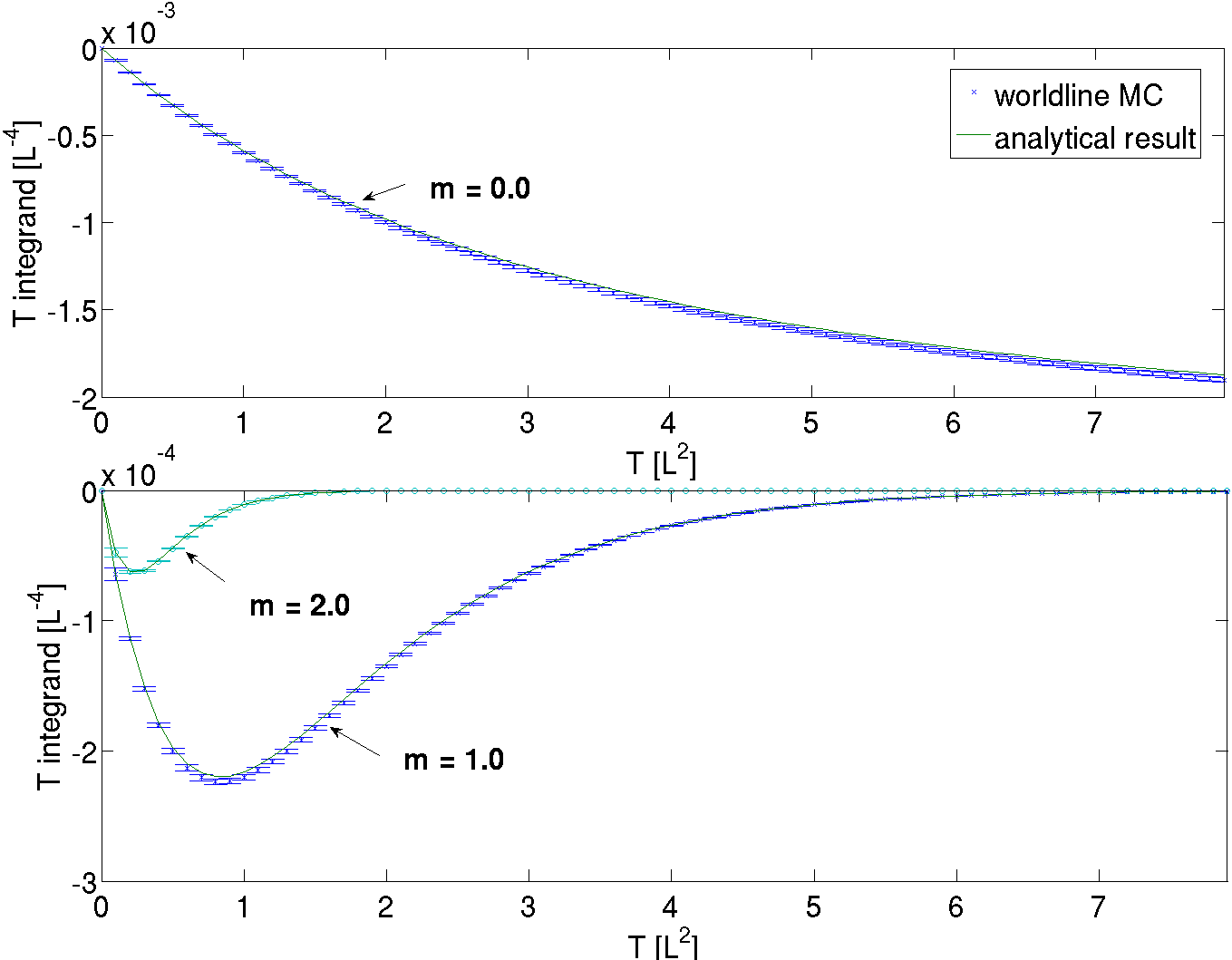
Figure 1: Comparison of the analytical and numerical results of the propertime integrands of Eqs. (III.1) and (III.1) for $k_{\mu}=(1,1,1,1)$ (in arbitrary inverse length units $L^{-1}$ and Lorentz indices chosen to point into the 11-direction for different values of the electron mass: $m=0$ (upper panel) and $m=1$ and $m=2$ (lower panel). In all cases, we have used the same ensemble of random worldlines. A test of the algorithm shows that an ensemble with $N_{\text{ppl}}=1000$, $n_{\text{L}}=40000$ gives us acceptable results with respect to both the calculation time and the numerical errors.

In Fig. 2, the diagonal (upper panel) and off-diagonal (lower panel) components of the vacuum polarization tensor in Euclidean space are shown as a function of the mass parameter $m$ again for the case $k_{\mu}=(1,1,1,1)$. The good agreement between analytical and numerical results for a wide range of mass values demonstrates that our method is capable of computing perturbative correlation functions with worldline numerics.

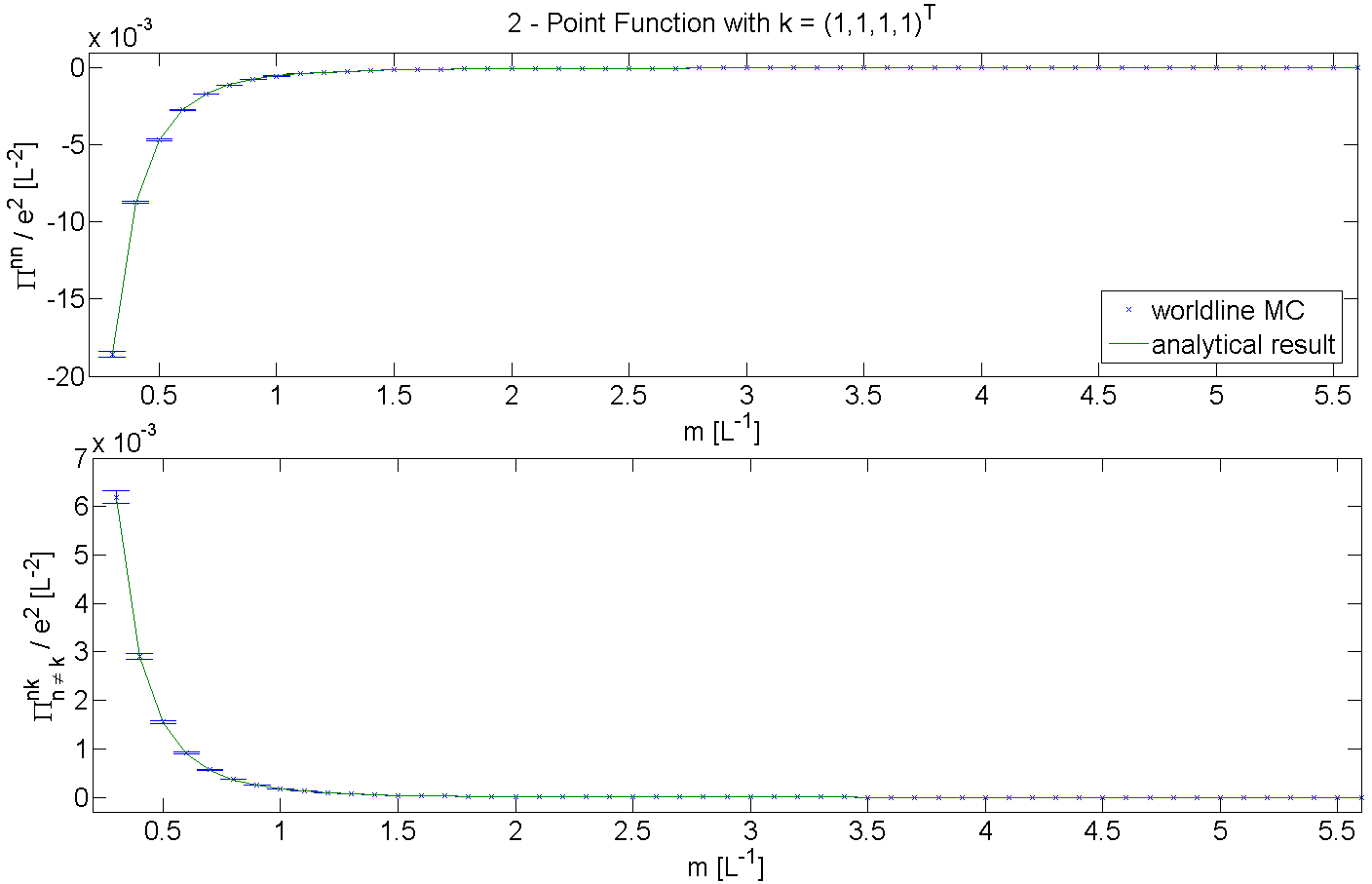
Figure 2: Comparison of the analytical and numerical results for the full polarization tensor $\Pi^{\mu\nu}$ in scalar QED as a function of the electron mass $m$. The upper panel depicts a generic result for the diagonal elements ($\mu=\nu$). The lower panel shows the same for off-diagonal elements.

As described above, we have performed the renormalization by polynomially fitting the propertime integrand and successively subtracting the counterterm corresponding to charge renormalization. More precisely, the term in curly brackets in Eq. (III.1) is fitted, for instance, to

$$P=bT+cT^{2}+dT^{3},$$ (16)

or higher-order polynomials. The algorithm can be stabilized by inserting the analytically known coefficients from the heat-kernel expansion, $b=-k^{2}/30$, $c=k^{4}/420$, $d=-k^{6}/7560$. Similar techniques and knowledge of the heat-kernel expansion can as well be employed in the case of nonvanishing electromagnetic fields.

IV Polarization tensor in a homogeneous magnetic field

As is obvious in the worldline approach, the generalization to nonvanishing background fields is straightforward, by inserting the Wegner-Wilson loop

$$e^{-ie\int_{0}^{T}d\tau\leavevmode\nobreak\ \dot{x}_{\mu}A^{\mu}(x(\tau))}.$$

into the worldline average in Eq. (III.1), cf. Eq. (13), with $x(\tau)=x_{\text{CM}}+\sqrt{T}y(t)$, $t=\tau/T$. As another test of our method, we compute the vacuum refractive indices arising from fluctuations in a homogeneous magnetic field. Due to homogeneity, the 4-momentum of the photon is conserved, implying $k_{1}+k_{2}=0$, such that we can directly study the polarization tensor. Writing the gauge potential in the form

$$A^{\mu}=\frac{1}{2}F^{\mu\nu}\dot{x}_{\nu}=\frac{1}{2}B\Lambda^{\mu\nu}\dot{x}_{\nu}$$

with the magnetic field strength $B$ and a dimensionless 4-dimensional tensor $\Lambda^{\mu\nu}$. Choosing the magnetic field to point into the $\mathbb{e}_{1}$ direction, $\Lambda^{\mu\nu}$ in Euclidean as well as in Minkowski space reads:

$$\Lambda=\left(\begin{matrix}0&0&0&0\\ 0&0&1&0\\ 0&-1&0&0\\ 0&0&0&0\end{matrix}\right).$$

The refractive indices are the inverse of the phase velocities of photons propagating in a magnetized quantum vacuum. As the magnetic field distinguishes a direction in space, the magnetized quantum vacuum is birefringent like a uniaxial crystal, featuring two polarization dependent phase velocities,

$$v_{\|/\perp}^{2}=1-\frac{\Pi_{\|,\perp}}{\mathbb{k}^{2}}=(1-\Delta v_{\|/\perp})^{2},$$ (17)

where $\Pi_{\|,\perp}$ are the nontrivial eigenvalues of the eigenmodes $\epsilon_{\mu}$ of the polarization tensor Dittrich:2000zu , $\Pi^{\mu\nu}\epsilon_{\mu,\|/\perp}=\Pi_{\|/\perp}\epsilon_{\mu,\|/\perp}$ satisfying the Minkowski-space photon dispersion relation

$$k^{2}+\Pi_{\|/\perp}=0.$$ (18)

Equations (17) and (18) are actually identical as the phase velocity is defined as $v=\omega/|\mathbf{k}|$. Here, we use the Minkowski metric $g=(-,+,+,+)$ and parameterize the Minkowskian momentum as $(k^{\mu})_{\text{M}}=(\omega,|\mathbf{k}|)$. For scalar QED, the velocity shifts, $\Delta v_{\|/\perp}=1-v_{\|,\perp}$ in the weak-field limit yield Ahlers:2006iz

$$\Delta v_{\|/\perp}=a_{\|/\perp}\frac{\alpha}{(4\pi)}\frac{(eB)^{2}}{m^{4}}\sin^{2}\theta,\quad a_{\|/\perp}=\left\{\begin{matrix}\frac{1}{90}\\ \\ \frac{7}{90}\end{matrix}\right\}.$$ (19)

Here $\theta$ denotes the angle spanned by the magnetic field $\mathbf{B}$ and the propagation direction $\mathbf{k}$. For weak fields, the $\|$ mode is polarized in the plane spanned by $\mathbf{B}$ and $\mathbf{k}$, whereas the $\perp$ mode is polarized orthogonal to this plane; more explicitly, $\epsilon_{\|}\sim\widetilde{\Lambda}k$ and $\epsilon_{\perp}\sim\Lambda k$, with $\widetilde{\Lambda}$ denoting the dual field strength matrix.

Even though the worldline numerical formalism is set up in Euclidean space, as the Monte Carlo procedure requires a positive action, extracting these light propagation properties obviously requires a transition to Minkowski space. In particular, we have to insert a Minkowski-valued 4-momentum vector into the worldline average to have access to real light-cone properties. We do so by choosing the Euclidean 4-momentum vector as $k_{\mu}=(i\omega,\mathbf{k})$. As illustrated in the Appendix, the algorithm remains stable at moderate frequencies, even though larger fluctuations require typically two orders of magnitude more statistics than typical Euclidean computations.

In Fig. 3, we compare our worldline Monte-Carlo results with those of the analytically known velocity shifts Ahlers:2006iz over a wider range of magnetic field strength (also exceeding the simple weak field limit). This benchmark test is performed for orthogonal incident $\theta=\pi/2$ and for the $\|$ mode at a frequency $\omega=0.1m$. The numerical results approach the velocity shift in the weak-field limit with very good accuracy and also yield reliable results for larger field strengths.

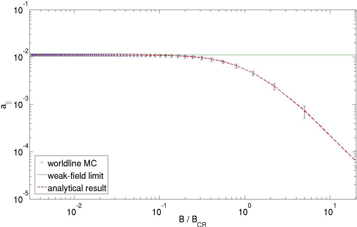
Figure 3: Benchmark test: velocity shift prefactor $a_{\|}$ in a homogeneous magnetic field for the $\|$ mode at orthogonal incident $\theta=\pi/2$ and for $\omega=0.1m$. For weak fields, $a_{\|}$ approaches the analytical result $1/90$ ($\approx 0.01111$), see Eq. (19). Also for larger fields, $a_{\|}$ follows the analytically known nonperturbative result Ahlers:2006iz .

V Polarization tensor in a spatially inhomogeneous magnetic field

Let us now explore new vacuum polarization effects in inhomogeneous fields, revealing the nonlocal nature of fluctuation-induced processes. For this, we use a magnetic background pointing into, say, $\mathbf{e}_{1}$ direction, consisting of a constant magnetic field $\overline{B}$ superimposed with a sinusoidal oscillation varying in $\mathbf{e}_{3}$ direction with amplitude $B_{1}$ and wavelength $\lambda_{B}$,

$$\mathbf{B}(x_{3})=\left[\overline{B}+B_{1}\cos\left(\frac{2\pi}{\lambda_{B}}x_{3}\right)\right]\mathbb{e}_{1}.$$ (20)

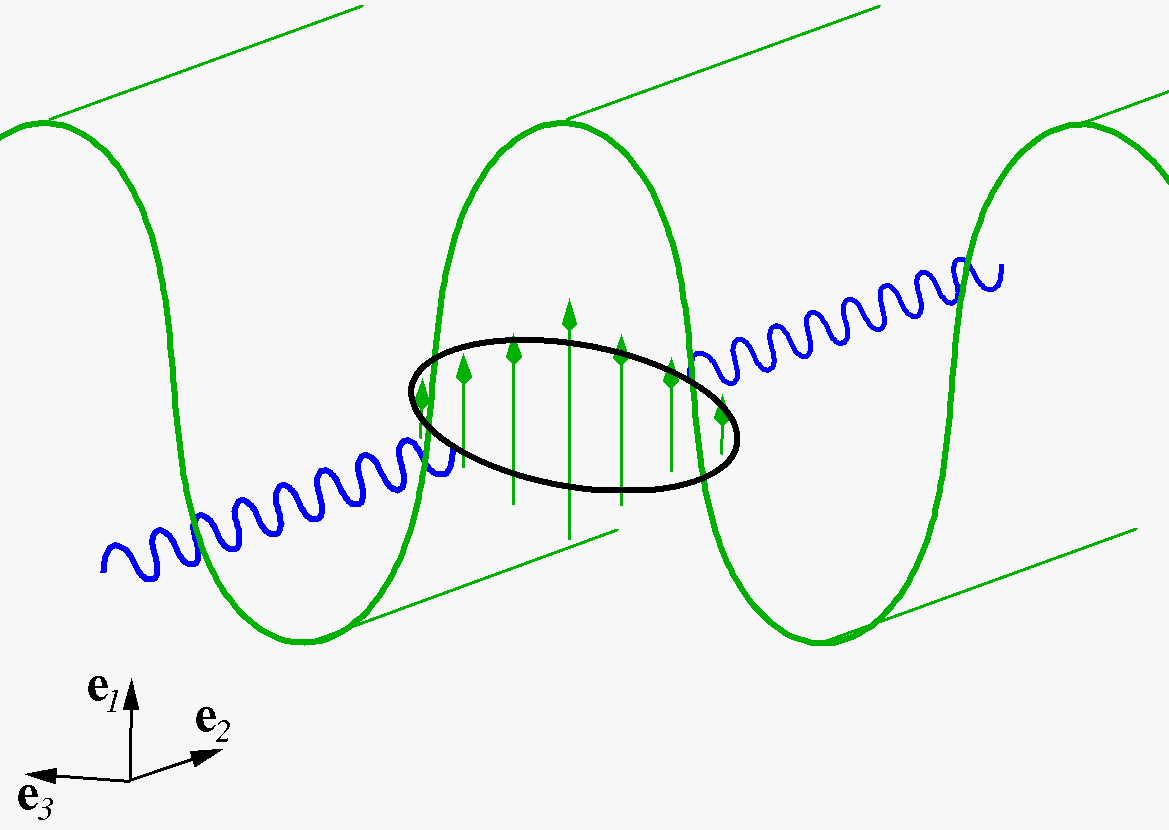
Figure 4: Sketch of the geometry of our configuration with an inhomogeneous magnetic field $\text{{B}}(x_{3})$ (green arrows and corrugated surface) with a constant magnetic component $\overline{B}$ in $\mathbf{e}_{1}$ direction and a spatial variation along the $\mathbf{e}_{3}$ direction with field amplitude $B_{1}$ also pointing into the $\mathbf{e}_{1}$ direction. The photon (blue wiggly line) propagates perpendicular to the field in $\mathbf{e}_{2}$ direction. The fluctuation-induced interaction between the photon and the magnetic field is represented by a Feynman diagram (black ellipse).

A similar electric field has already been used to analyze the role of spatial inhomogeneities in Schwinger pair production Gies:2005bz . This field configuration can be viewed as a rough approximation to a realistic strong and broad laser pulse in standing wave mode superposed with higher harmonics.

For the worldline simulation, we use the corresponding gauge potential

$$A_{2}=-\overline{B}x_{3}-\frac{B_{1}\lambda_{B}}{2\pi}\sin\left(\frac{2\pi}{\lambda_{B}}x_{3}\right),$$ (21)

which is numerically convenient, as it depends only on one spatial coordinate.

As a relevant observable, we compute the local velocity shift $\Delta v(x_{3})$ for a photon propagating along the $\mathbf{e}_{2}$ direction from the local polarization tensor. The geometry of our configuration is sketched in Fig. 4. As the magnetic field is homogeneous in $\mathbf{e}_{2}$ direction, the photon momentum is conserved $k_{1}+k_{2}=0$ for $\mathbf{k}_{1}\sim\mathbf{k}_{2}\sim\mathbf{e}_{2}$. Hence, setting $k=k_{1}=-k_{2}$ and inserting (21) into the local polarization tensor (13), we can determine $\pi^{\mu\nu}[k,x_{3,\text{CM}};A]$, which is diagonalized by the same polarization eigenmodes $\epsilon_{\mu,\|/\perp}$ as the in constant-field case. The local phase velocity shifts then are computed analogous to Eq. (17),

$$v_{\|/\perp}^{2}(x_{3,\text{CM}})=1-\frac{\pi_{\|,\perp}(x_{3,\text{CM}})}{\mathbb{k}^{2}}=(1-\Delta v_{\|/\perp}(x_{3,\text{CM}}))^{2},$$ (22)

where $\pi_{\|,\perp}(x_{3,\text{CM}})$ are the local eigenvalues of the polarization tensor.

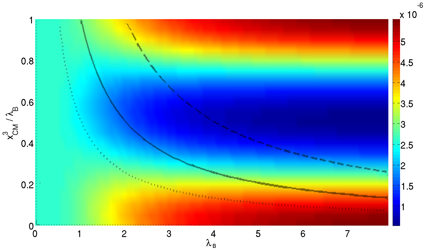
Figure 5: Contour plot of the phase velocity shift $\Delta v$ for an incoming $\|$-photon at orthogonal incident with respect to the direction of the external field ($\theta=\frac{\pi}{2}$). The inhomogeneous field has a sinusoidal variation along the $\mathbf{e}_{3}$ direction, cf. Eq. (20), with $e\overline{B}=0.2m^{2}$ and $B_{1}=0.5\overline{B}$. The phase velocity is plotted horizontally versus the oscillation wavelength $\lambda_{B}$ and vertically versus the normalized position $x_{3,\text{CM}}/\lambda_{B}$ of the photon relative to the oscillation phase. Lines of constant absolute position $x_{3,\text{CM}}=0.5,1.0,2.0$ in units of mass $m$ for varying wavelength $\lambda_{B}$ are indicated as dotted, solid and dashed lines.

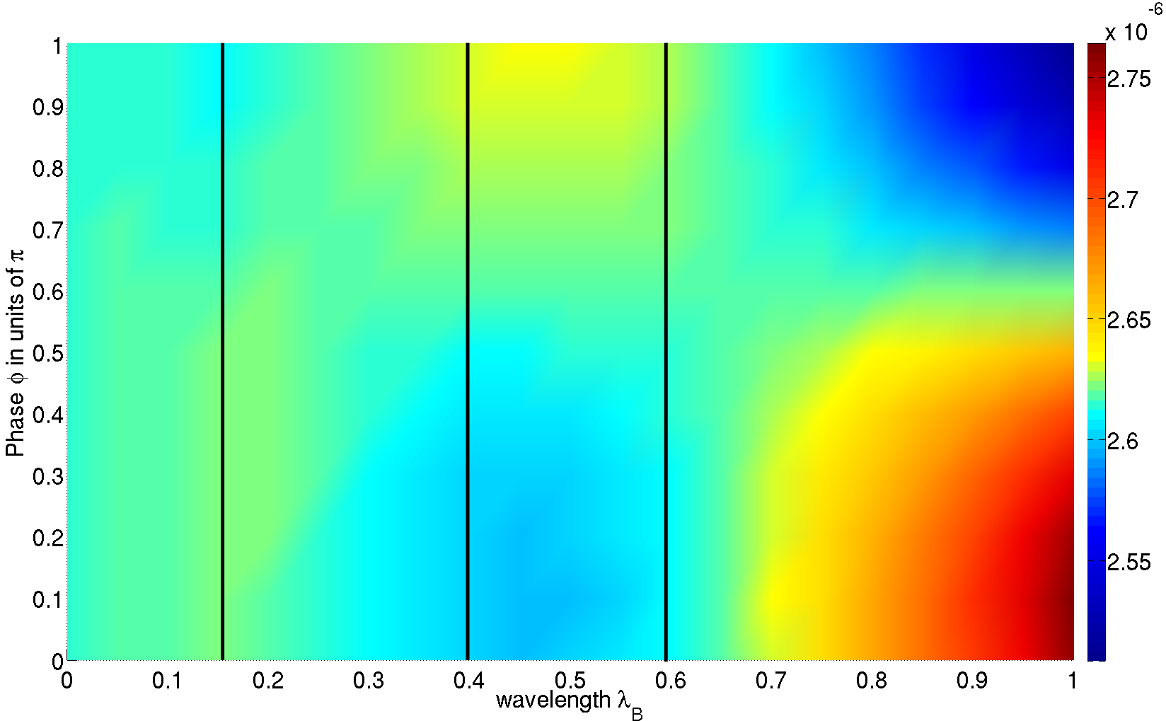
Figure 6: Contour plot with the same physical parameters as in Figure 5 but with a higher resolution in the region of small $\lambda_{B}$. The $y$ axis is now given in terms of the phase in units of $\pi$, $\phi/\pi=2x_{\text{CM}}/\lambda_{B}$. The straight lines are cuts at $\lambda=0.15,0.4,0.6$, which we discuss in Figure 8.

In our computation, we use $e\overline{B}=0.2m^{2}$ and $B_{1}=0.5\overline{B}$. Figure 5 shows a contour plot of the local velocity shift as a function of the oscillation wavelength $\lambda_{B}$ and the normalized coordinate $x_{3,\text{CM}}/\lambda_{B}$ for the $\|$-mode; the latter corresponds to the phase inside the oscillation period, $\phi=2\pi x_{3,\text{CM}}/\lambda_{B}$. For large $\lambda_{B}$ when the field becomes slowly varying with respect to the Compton wavelength $\lambda_{B}m\gg 1$, the local velocity shifts approach the constant field values as expected. A “locally-constant-field” approximation becomes reliable in this limit. By contrast, if the two characteristic length scales become similar $\lambda_{B}m\simeq 1$ the oscillating structure of the magnetic field starts to become washed out in the local velocity shift. The propagating photon undergoing virtual electron-positron loops with an inherent length scale of the Compton wavelength “sees” a field averaged over this length scale. For a rapidly oscillating field, $\lambda_{B}m\ll 1$, the field oscillations are completely washed out and become invisible in the velocity shift. In our present example, the limiting velocity shift in this rapid-oscillation limit corresponds precisely to that induced by the background field $\overline{B}$, $\Delta v\sim\overline{B}^{2}$. This is in line with the interpretation that the averaging arises from the nonlocal nature of the fluctuations. For instance, naively averaging over the constant-field velocity shift, depending quadratically on $B$, would give a different (and wrong) averaging result, $\Delta v\not\sim(\overline{B}^{2}+\frac{1}{2}B_{1}^{2})$.

An interesting parameter regime occurs at small $\lambda_{B}$, i.e., for rapidly varying background field, see Fig. 6. In Fig. 7, we show horizontal slices of the contour plot Fig. 6 at the ordinate values $x_{3,\text{CM}}/\lambda_{B}=0,0.25,0.5$, corresponding to different positions in the phase of the variation $\phi/\pi=2x_{3,\text{CM}}/\lambda_{B}=0,0.5,1$, as a function of the variation length $\lambda_{B}$. For large $\lambda_{B}$, the velocity shifts approach their constant-field limits with a clear ordering from large to small background field from top to bottom. This is in accordance with expectations from a locally-constant-field approximation becoming applicable for large $\lambda_{B}$.

By contrast, this ordering is lost at small $\lambda_{B}$, where the curves show a characteristic oscillation pattern, see inlay of Fig. 7. Depending on the value of $\lambda_{B}$, the velocity shift in a local minimum of the field (red stars, $\phi/\pi=1$) can become larger than that in a local maximum (blue dots, $\phi/\pi=0$), cf. inlay of Fig. 7 at around $\lambda_{B}\simeq 0.65$.

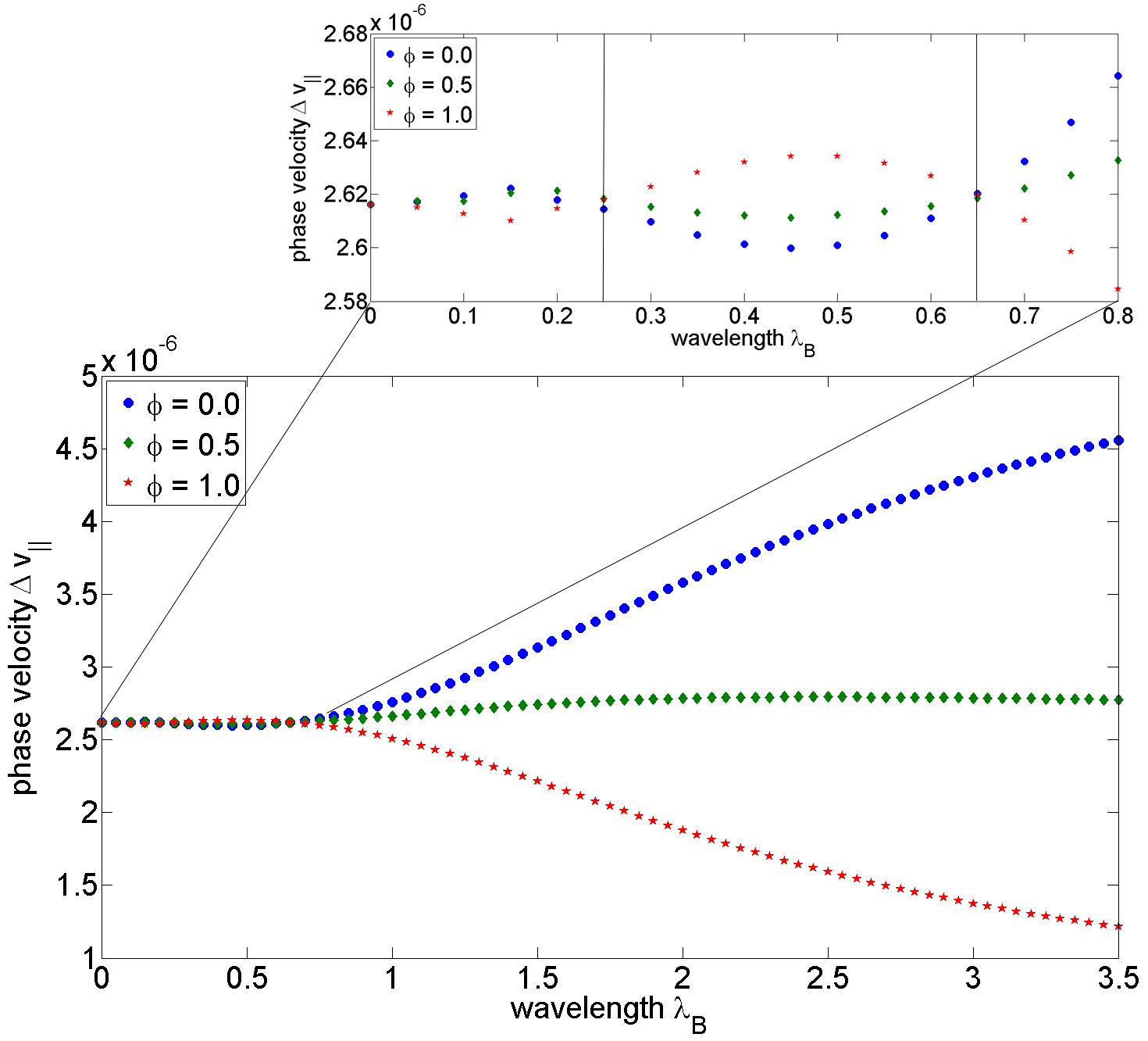
Figure 7: Phase velocity shift $\Delta v_{\|}$ for different positions in the phase of the variation $\phi=2\pi x_{3,\text{CM}}/\lambda_{B}$ as a function of the variation length $\lambda_{B}$. The curves correspond to horizontal slices of the contour plot Figs. 5,6 at the ordinate values $\phi/\pi=2x_{\text{CM}}/\lambda_{B}=0,0.5,1$. For large $\lambda_{B}$, the velocity shifts approach their constant-field limits with a clear ordering from large to small background field from top to bottom (blue dots at field maximum to red stars at minimum field). By contrast, this ordering is modified at small $\lambda_{B}$ in various patterns depending on the value of $\lambda_{B}$ (see inlay). The straight lines in the inlay at $\lambda_{B}\simeq 0.25,0.65$ mark the turning points.

We interpret this phenomenon as a consequence of the local averaging property of the quantum fluctuations on scales of the Compton wavelength $m$. In this way, the local velocity shift in a minimum of the field can receive dominant contributions from the nearby maxima if they are significantly probed by the quantum fluctuations on the scale $1/m$. Conversely, the local velocity shift in a maximum of the field can receive dominant contributions from the nearby minima. This can lead to an inversion of the hierarchy of the velocity shifts with respect to the local background field. Our data is compatible with further oscillations setting in at even smaller values of $\lambda_{B}\simeq 0.25$, which would correspond to further minima or maxima entering the local fluctuation average.

variation length $\lambda_{B}$	amplitude $A$	phase shift $\phi_{0}/\pi$	constant velocity shift $\Delta v_{0}$
0.15	7.36$\cdot 10^{-9}\pm$2.5$\cdot 10^{-9}$	0.31$\pm$0.30	2.62$\cdot 10^{-6}\pm$3.4$\cdot 10^{-8}$
0.40	1.61$\cdot 10^{-8}\pm$4.8$\cdot 10^{-8}$	1.09$\pm$5.4$\cdot 10^{-1}$	2.62$\cdot 10^{-6}\pm$5.1$\cdot 10^{-8}$
0.60	8.66$\cdot 10^{-9}\pm$3.4$\cdot 10^{-8}$	1.13$\pm$6.8$\cdot 10^{-1}$	2.62$\cdot 10^{-6}\pm$5.1$\cdot 10^{-8}$
2.00	8.52$\cdot 10^{-7}\pm$2.1$\cdot 10^{-7}$	0.02$\pm$3.0$\cdot 10^{-2}$	2.74$\cdot 10^{-6}\pm$3.8$\cdot 10^{-8}$

Table 1: Fit parameters deduced from the numerical results of Fig. 8 using a least-squares fit to Eq. (23). Starting from large $\lambda_{B}$ (slowly varying field), the velocity shift is in phase with the external field, $\phi_{0}\simeq 0$. For $\lambda_{B}=0.4,0.6$, we observe a jump of the phase by $\phi_{0}/\pi\simeq 1$. For an even smaller variation scale $\lambda_{B}=0.15$ the phase $\phi_{0}$ goes back to values compatible with zero (the deviations from zero arise from the comparatively large signal to noise ratio of our data for small $\lambda_{B}$; this is also reflected in the large error bars for the amplitude $A$ for smaller $\lambda_{B}$).

This becomes visible in vertical slices of the contour plot Fig. 6 at the abscissa values $\lambda_{B}=0.15,0.4,0.6$, and $2$ as a function of the phase of the field variation $\phi=2\pi x_{3,\text{CM}}/\lambda_{B}$. In Fig. 8, we show the varying part of the velocity shift normalized by the maximum oscillation amplitude $A$. We observe the expected $2\pi$-periodicity of the phase velocity with respect to $\phi$. Most importantly, the oscillation is shifted by an offset $\phi_{0}=\pi$ for small wavelengths, e.g., $\lambda_{B}=0.4,0.6$, compared to larger $\lambda_{B}=2$ where the velocity shift tends to approach the locally-constant-field limit. This implies that velocity shift minima occur at field maxima and vice versa in the range $0.25\lesssim\lambda_{B}\lesssim 0.65$. For even more rapid field oscillations $\lambda_{B}\lesssim 0.25$, our data is compatible with the velocity shift being in phase with the external field again. This goes hand in hand with our interpretation in terms of fluctuation averages. The full Monte Carlo data can be parametrized by a simple fit,

$$f(x)=A\cos\left(2\pi\frac{x_{\text{CM}}}{\lambda_{B}}-\phi_{0}\right)+\Delta v_{0}.$$ (23)

The fitting results are given in Tab. 1.

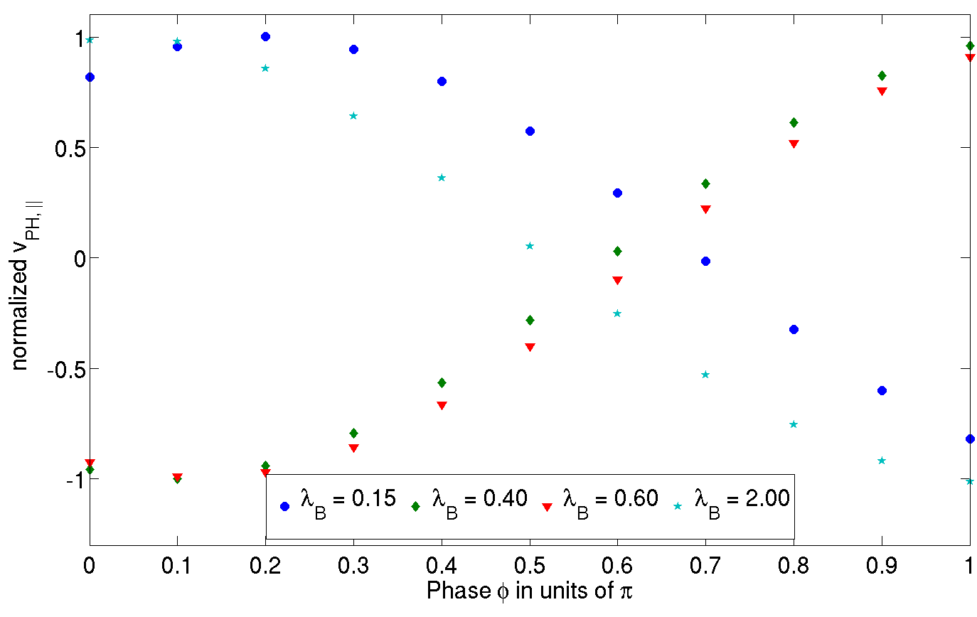
Figure 8: Normalized phase velocity shift $\Delta v_{\|}$ for different field inhomogeneities $\lambda_{B}=0.15,0.40,0.6,2.0$ as a function of the phase of the field variation $\phi/\pi=2x_{3,\text{CM}}/\lambda_{B}$. The curves correspond to vertical slices of the contour plot Fig. 6 at the given abscissa values for $\lambda_{B}$. The picture shows the expected $2\pi$-periodicity of the phase velocity with respect to $\phi$. For large $\lambda_{B}=2$ (light blue stars), the velocity shift is in phase with the background field $\sim\cos\phi$ as expected from a locally-constant field approximation. For $\lambda_{B}=0.4,0.6$ (green diamongs, red triangles), the velocity shift oscillates out of phase $\sim\cos(\phi-\phi_{0}$ with $\phi_{0}\simeq\pi$. For even smaller variation length $\lambda_{B}=0.15$, the oscillation is approximately in phase again $\sim\cos\phi$.

A similar phenomenon had already been observed for the case of pair production in inhomogeneous fields Gies:2005bz ; however, due to the exponential dependence of pair production on the background field, this averaging phenomenon was much more pronounced in this case. In fact, the amplitude of the oscillations is on the order of our statistical error bars for the velocity shift data. However, fitting the data at fixed $\lambda_{B}$ to sinusoidal fit functions translates into a correspondingly large error for the amplitude, but a significantly small error for the phase of the oscillation, see Tab.1. The size of our statistical errors can also be estimated from the deviations from symmetry about the horizontal $x_{3,\text{CM}}/\lambda_{B}=0.5$ axis in Fig. 5 or from anti-symmetry about the horizontal $\phi=0.5$ axis in Fig. 6. This latter anti-symmtry also guarantees that the exact result for the phase velocity shift at $\phi=0.5$ should not depend on $\lambda_{B}$; the slight dependence of the Monte Carlo data for the $\phi=0.5$ curve (green diamonds) on $\lambda_{B}$, hence is a measure for our statistical error.

As these velocity shifts correspond to shifts of the local refractive indices this new phenomenon has a direct consequence for the self-focussing property of the quantum vacuum Kharzeev:2006wg : in the locally-constant-field limit (a pure Heisenberg-Euler-type calculation), the refractive index increases with increasing field strength. This implies that photons are dragged into local maxima of the field strength. This even enhances the field strength at local maxima, thus giving rise to self-focussing properties. Our observation in turn predicts that this self-focussing naturally terminates on the scale of the Compton wavelength. If field maxima are self-focussed down to a critical scale $\lambda_{\text{cr,1}}$, field maxima with nearby minima can become local minima of the velocity shift (and thus minima of the local refractive index) such that the quantum vacuum becomes defocussing again. From the inlay of Fig. 7, we estimate this critical scale to be near $\lambda_{\text{cr,1}}\simeq 0.65$ in units of the Compton wavelength. This critical scale provides a natural limit to the self-focussing property of the quantum vacuum. As our data is compatible with an in-phase dependence of the refractive index on the field inhomogeneities for $\lambda_{B}\lesssim 0.25$, the quantum vacuum may become self-focussing again on this shorter variation scale. But this regime is also expected to terminate at another critical scale $\lambda_{\text{cr,2}}$ where the velocity shift may run out of phase again. Our data is compatible with $\lambda_{\text{cr,2}}\lesssim 0.05$.

VI Conclusions

Based on the successful worldline approach to perturbative correlation functions, we have developed numerical Monte-Carlo techniques for the computation of the vacuum polarization tensor in inhomogeneous background fields for scalar QED. These techniques generalize earlier methods which have been frequently applied to effective action or quantum energy computations. The new challenge in the case of correlation functions is the appearance of further scales provided by the incoming and outgoing momenta.

The stability of the numerical algorithm also originates in the fact that it satisfies the Ward identity exactly and operates on the level of renormalized quantities. We have explicitly demonstrated that the algorithm can also be used to determine correlation functions as a function of Minkowski-valued momenta and fields, even though stability is expected to become an issue for increasing Minkowski momenta or dominating electric field components.

We have verified our algorithm with the analytically known cases of the vacuum polarization tensor for off-shell momenta and the polarization tensor in homogeneous fields using the magnetically induced light-cone deformations as an observable. In these cases, the algorithm is capable to reach a precision on the percent level at moderate numerical cost.

Furthermore, we have studied for the first time light propagation in a spatially varying magnetic field. For small variations of the field compared to the Compton wavelength, the local derivative expansion (or locally-constant-field approximation) is well applicable as expected, such that the vacuum polarization tensor quickly approaches the constant-field limit.

For rapidly varying fields, the vacuum-magnetic refractive indices can exhibit a non-monotonic dependence on the local field strength. This new behavior can geometrically be understood in the worldline picture, as the worldlines and their spatial extent probes the nonlocal structure of quantum field theory. Local values of the refractive indices can receive dominant contributions from nearby maxima or minima of the field strength. This inherent averaging mechanism induces a smearing and even non-monotonical features of the refractive indices. For the properties of light propagation, this can provide a natural limit on the self-focussing property of the quantum vacuum.

Our present study represents a first step into the largely unknown territory of quantum correlation functions in inhomogeneous fields. Even though we have concentrated on the two-point function in the present work, we expect that our algorithmic strategy can rather straightforwardly be generalized to higher-order correlation functions. Also a generalization to spinor QED is in principle straightforward and merely requires the inclusion of the worldline spin factor involving a numerically moderately expensive path-ordering prescription.

Appendix A Validity control of the numerical algorithm

The worldline Monte Carlo method has proven its efficiency and accuracy in many examples in the context of effective action and quantum energy computations. Generically, the convergence is very satisfactory and scales with a typical Monte Carlo $1/\sqrt{n_{\text{L}}}$ dependence, where $n_{\text{L}}$ is the number of configurations, i.e., worldlines in this case. Precision with an error on the 1% level can be achieved with moderate numerical cost. In the present case, it is worthwhile to critically re-examine the quality and efficiency of the algorithm, as the calculation of correlation functions goes along with further technical requirements. Most prominently, the physical observables need to be computed with Minkowski-valued momenta which technically is a potential source of numerical instability. This is because the Euclidean phase factors $\sim\exp(ik_{\mu}x_{\mu})$ receive real exponential contributions for Minkowskian momenta $k_{0}\to i\omega$. Also, the frequency and spatial momentum dependence introduces further scales which can interfere with the scale of inhomogeneity.

All error estimates in this work are based on the Jackknife method. We have checked explicitly, that this error estimate using the same random number seed yields results equivalent to an error estimate derived from a set of ensembles created with different random number seeds.

In Fig. 9, we compare the relative error for the velocity shift $\Delta v_{\|}$ in percent as a function of the number of worldline configurations $n_{\text{L}}$ for various parameters. The smallest error is observed for a purely Euclidean constant field calculation (green dots). This type of calculation is closest to conventional effective action and quantum energy computations; however, in the present case it does not describe a physical observable. The corresponding physical Minkowskian calculation for the constant-field case (blue diamonds) shows an error increase of roughly an order of magnitude. This implies that an error on the level of a typical Euclidean calculation requires two orders of magnitude more statistics.

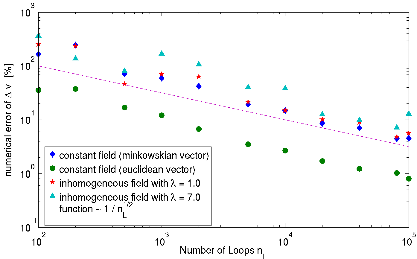
Figure 9: Relative error (jackknife estimate) for the velocity shift $\Delta v$ in percent as a function of $n_{\text{L}}$ for a Euclidean vs. Minkowskian calculation including its dependence on the field inhomogeneity. We have used a worldline ensemble with $N=1000$ points per loop. The plot shows a comparison between the Euclidean constant-field case with $e\overline{B}/m^{2}=0.2$ and a Minkowskian calculation for the same constant-field case (blue diamonds). Two Minkowskian calculations for the inhomogeneous field of Sect. V with wavelengths $\lambda_{B}=1.0$ (red stars) and $\lambda_{B}=7.0$ (light blue triangles) are also shown. Because of the stronger fluctuations in the Minkowskian case, all Minkowskian calculations show larger relative errors. The dependence of the error on the background inhomogeneity is comparatively minor. For illustration, also a line $\sim 1/\sqrt{n_{\text{L}}}$ is shown reflecting the expected error depletion for Monte Carlo calculations.

The interference of the error with the external scales is also illustrated in Fig. 9, where we determine the relative error for the velocity shift $\Delta v$ in percent as a function of $n_{\text{L}}$ and its dependence on the field inhomogeneity for two different values $\lambda_{B}$ parameterizing the field inhomogeneity. Even though we observe some dependence on the field inhomogeneity leading to slightly larger errors, the main effect on the error clearly arises from the necessity to perform Minkowski-valued calculations.

Fig. 9 also depicts a straight line exhibiting a $\sim 1/\sqrt{n_{\text{L}}}$ dependence in this double-log plot. This indicates that the numerical error decreases with increasing number of worldlines $n_{\text{L}}$ as $\sim 1/\sqrt{n_{\text{L}}}$, as expected. Even for these perturbatively small Minkowski-valued quantities, errors below the 10% level are achievable at managable numerical cost.

References

- (1) J. S. Toll, Ph.D. thesis, Princeton Univ., 1952 (unpublished).
- (2) R. Baier and P. Breitenlohner, Act. Phys. Austriaca 25, 212 (1967); Nuov. Cim. B 47 117 (1967).
- (3) Z. Bialynicka-Birula and I. Bialynicki-Birula, Phys. Rev. D 2, 2341 (1970).
- (4) S. L. Adler, Annals Phys. 67, 599 (1971).
- (5) W. y. Tsai and T. Erber, Phys. Rev. D 12, 1132, (1975).
- (6) H. Gies, Phys. Rev. D 61, 085021 (2000).
- (7) W. Dittrich and H. Gies, Springer Tracts Mod. Phys. 166, 1 (2000).
- (8) W. y. Tsai and T. Erber, Phys. Rev. D 10, 492 (1974).
- (9) J. K. Daugherty and A. K. Harding, Astrophys. J. 273, 761 (1983).
- (10) R. Cameron et al. [BFRT Collaboration], Phys. Rev. D 47 (1993) 3707.
- (11) E. Zavattini et al. [PVLAS Collaboration], arXiv:0706.3419 [hep-ex].
- (12) S. J. Chen, H. H. Mei and W. T. Ni, Mod. Phys. Lett. A 22, 2815 (2007) [arXiv:hep-ex/0611050].
- (13) C. Robilliard et al., Phys. Rev. Lett. 99, 190403 (2007); F. Bielsa et al., arXiv:0911.4567 [physics.optics].
- (14) P. Pugnat et al., CERN-SPSC-2006-035, CERN-SPSC-P-331, (2006); P. Pugnat et al. [OSQAR Collaboration], Phys. Rev. D 78, 092003 (2008) [arXiv:0712.3362 [hep-ex]].
- (15) L. Maiani, R. Petronzio and E. Zavattini, Phys. Lett. B 175, 359 (1986); G. Raffelt and L. Stodolsky, Phys. Rev. D 37, 1237 (1988).
- (16) H. Gies, J. Jaeckel and A. Ringwald, Phys. Rev. Lett. 97, 140402 (2006) [arXiv:hep-ph/0607118];
- (17) M. Ahlers, H. Gies, J. Jaeckel and A. Ringwald, Phys. Rev. D 75, 035011 (2007).
- (18) M. Ahlers, H. Gies, J. Jaeckel, J. Redondo and A. Ringwald, Phys. Rev. D 76, 115005 (2007); Phys. Rev. D 77, 095001 (2008) [arXiv:0711.4991 [hep-ph]].
- (19) T. Heinzl et al., Opt. Commun. 267, 318 (2006) [arXiv:hep-ph/0601076].
- (20) B. Marx, et al., Opt. Commun. 284, 915 (2011).
- (21) A. Di Piazza, K. Z. Hatsagortsyan and C. H. Keitel, Phys. Rev. D 72, 085005 (2005); A. Di Piazza, K. Z. Hatsagortsyan and C. H. Keitel, Phys. Rev. Lett. 97, 083603 (2006) [arXiv:hep-ph/0602039]. A. Di Piazza, A. I. Milstein and C. H. Keitel, arXiv:0704.0695 [hep-ph]; . C. Muller, A. Di Piazza, A. Shahbaz, T. Burvenich, J. Evers, K. Hatsagortsyan and C. Keitel, Laser Phys. 18, 175 (2008).
- (22) R. Schutzhold, H. Gies and G. Dunne, Phys. Rev. Lett. 101, 130404 (2008) [arXiv:0807.0754 [hep-th]]; G. V. Dunne, H. Gies and R. Schutzhold, Phys. Rev. D 80, 111301 (2009) [arXiv:0908.0948 [hep-ph]]; M. Ruf, G. R. Mocken, C. Muller, K. Z. Hatsagortsyan and C. H. Keitel, Phys. Rev. Lett. 102, 080402 (2009) [arXiv:0810.4047 [physics.atom-ph]]; T. Heinzl, A. Ilderton and M. Marklund, arXiv:1002.4018 [hep-ph].
- (23) A. Di Piazza, E. Lotstedt, A. I. Milstein and C. H. Keitel, Phys. Rev. Lett. 103, 170403 (2009) [arXiv:0906.0726 [hep-ph]]; S. S. Bulanov, V. D. Mur, N. B. Narozhny, J. Nees and V. S. Popov, Phys. Rev. Lett. 104, 220404 (2010) [arXiv:1003.2623 [hep-ph]]; M. Orthaber, F. Hebenstreit and R. Alkofer, arXiv:1102.2182 [hep-ph].
- (24) F. Hebenstreit, R. Alkofer, G. V. Dunne and H. Gies, Phys. Rev. Lett. 102, 150404 (2009) [arXiv:0901.2631 [hep-ph]]; arXiv:0910.4457 [hep-ph].
- (25) F. Mackenroth, A. Di Piazza and C. H. Keitel, Phys. Rev. Lett. 105, 063903 (2010) [arXiv:1001.3614 [physics.acc-ph]]; C. K. Dumlu and G. V. Dunne, “The Stokes Phenomenon and Schwinger Vacuum Pair Production in Phys. Rev. Lett. 104, 250402 (2010) [arXiv:1004.2509 [hep-th]].
- (26) D. Tommasini, A. Ferrando, H. Michinel and M. Seco, JHEP 0911, 043 (2009) [arXiv:0909.4663 [hep-ph]].
- (27) B. King, A. Di Piazza, and C.H. Keitel, Nature Photon. 4, 92 (2010).
- (28) D. B. Blaschke, G. Roepke, V. V. Dmitriev, S. A. Smolyansky and A. V. Tarakanov, arXiv:1101.6021 [physics.plasm-ph]; G. Gregori et al., High Energy Dens. Phys. 6, 166 (2010) [arXiv:1005.3280 [hep-ph]].
- (29) C. Harvey, T. Heinzl, A. Ilderton, Phys. Rev. A79, 063407 (2009). [arXiv:0903.4151 [hep-ph]]; T. Heinzl, D. Seipt, B. Kampfer, Phys. Rev. A81, 022125 (2010). [arXiv:0911.1622 [hep-ph]].
- (30) M. Marklund and J. Lundin, Eur. Phys. J. D 55, 319 (2009) [arXiv:0812.3087 [hep-th]].
- (31) G. V. Dunne, Eur. Phys. J. D 55, 327 (2009) [arXiv:0812.3163 [hep-th]].
- (32) T. Heinzl, A. Ilderton, Eur. Phys. J. D55, 359-364 (2009). [arXiv:0811.1960 [hep-ph]].
- (33) H. Gies, Eur. Phys. J. D 55, 311 (2009) [arXiv:0812.0668 [hep-ph]].
- (34) K. Homma, D. Habs and T. Tajima, arXiv:1006.4533 [quant-ph].
- (35) B. Dobrich and H. Gies, JHEP 1010, 022 (2010) [arXiv:1006.5579 [hep-ph]]; B. Dobrich and H. Gies, arXiv:1010.6161 [hep-ph].
- (36) T. Heinzl, A. Ilderton, M. Marklund, Phys. Rev. D81, 051902 (2010). [arXiv:0909.0656 [hep-ph]].
- (37) I. A. Batalin and A. E. Shabad, Zh. Eksp. Teor. Fiz. 60, 894 (1971).
- (38) V. I. Ritus, “Radiative corrections in quantum electrodynamics with intense field and Annals Phys. 69, 555 (1972).
- (39) R. A. Cover and G. Kalman, Phys. Rev. Lett. 33, 1113 (1974).
- (40) L. F. Urrutia, Phys. Rev. D 17, 1977 (1978).
- (41) G. K. Artimovich, “Properties of the photon polarization operator in an electric field: Sov. Phys. JETP 70, 787 (1990) [Zh. Eksp. Teor. Fiz. 97, 1393 (1990)].
- (42) C. Schubert, Nucl. Phys. B 585, 407 (2000) [arXiv:hep-ph/0001288].
- (43) W. Dittrich and R. Shaisultanov, Phys. Rev. D 62, 045024 (2000) [arXiv:hep-th/0001171].
- (44) S. Konar, Int. J. Mod. Phys. A 17, 1055 (2002) [arXiv:hep-ph/0111104].
- (45) S. Villalba-Chavez, Phys. Lett. B 692, 317 (2010) [arXiv:1008.0547 [hep-th]].
- (46) A. I. Nikishov, Nucl. Phys. B 21, 346 (1970).
- (47) D. Cangemi, E. D’Hoker and G. V. Dunne, Phys. Rev. D 52, 3163 (1995) [arXiv:hep-th/9506085].
- (48) S. P. Kim and D. N. Page, Phys. Rev. D 65, 105002 (2002) [arXiv:hep-th/0005078].
- (49) M. B. Halpern, A. Jevicki and P. Senjanovic, “Field Theories In Terms Of Particle-String Variables: Spin, Internal Phys. Rev. D 16, 2476 (1977); Z. Bern and D. A. Kosower, Nucl. Phys. B 379, 451 (1992).
- (50) M. J. Strassler, Nucl. Phys. B 385, 145 (1992) [arXiv:hep-ph/9205205];
- (51) M. G. Schmidt and C. Schubert, Phys. Lett. B 318, 438 (1993) [arXiv:hep-th/9309055].
- (52) C. Schubert, Phys. Rept. 355, 73 (2001) [arXiv:hep-th/0101036].
- (53) H. Gies and K. Langfeld, Nucl. Phys. B 613, 353 (2001) [arXiv:hep-ph/0102185]; Int. J. Mod. Phys. A 17, 966 (2002) [arXiv:hep-ph/0112198].
- (54) K. Langfeld, L. Moyaerts and H. Gies, Nucl. Phys. B 646, 158 (2002) [arXiv:hep-th/0205304].
- (55) H. Gies and K. Klingmuller, Phys. Rev. D 72, 065001 (2005) [arXiv:hep-ph/0505099].
- (56) H. Gies, K. Langfeld and L. Moyaerts, JHEP 0306, 018 (2003) [arXiv:hep-th/0303264]; H. Gies and K. Klingmuller, Phys. Rev. Lett. 97, 220405 (2006) [arXiv:quant-ph/0606235]; A. Weber and H. Gies, Phys. Rev. Lett. 105, 040403 (2010) [arXiv:1003.0430 [hep-th]].
- (57) G. Dunne, H. Gies, K. Klingmuller and K. Langfeld, JHEP 0908, 010 (2009) [arXiv:0903.4421 [hep-th]].
- (58) D. Kharzeev and K. Tuchin, Phys. Rev. A 75, 043807 (2007) [arXiv:hep-ph/0611133].
- (59) H. Gies, J. Sanchez-Guillen and R. A. Vazquez, JHEP 0508, 067 (2005) [arXiv:hep-th/0505275].