Collisional rates for the inelastic Maxwell model: application to the divergence of anisotropic high-order velocity moments in the homogeneous cooling state

Abstract

The collisional rates associated with the isotropic velocity moments $\langle V^{2r}\rangle$ and the anisotropic moments $\langle V^{2r}V_{i}\rangle$ and $\langle V^{2r}(V_{i}V_{j}-d^{-1}V^{2}\delta_{ij})\rangle$ are exactly derived in the case of the inelastic Maxwell model as functions of the exponent $r$, the coefficient of restitution $\alpha$, and the dimensionality $d$. The results are applied to the evolution of the moments in the homogeneous free cooling state. It is found that, at a given value of $\alpha$, not only the isotropic moments of a degree higher than a certain value diverge but also the anisotropic moments do. This implies that, while the scaled distribution function has been proven in the literature to converge to the isotropic self-similar solution in well-defined mathematical terms, nonzero initial anisotropic moments do not decay with time. On the other hand, our results show that the ratio between an anisotropic moment and the isotropic moment of the same degree tends to zero.

1 Introduction

The prototypical model of a granular gas consists of a system of (smooth) inelastic hard spheres (IHS) with a constant coefficient of normal restitution $0<\alpha\leq 1$ BP04 . Under low-density conditions, the one-particle velocity distribution function $f(\mathbf{r},\mathbf{v};t)$ obeys the (inelastic) Boltzmann equation. On the other hand, because of the intricacy of the collision operator, one has to resort to approximate or numerical methods to get explicit results, even in the elastic case ($\alpha=1$). The main mathematical difficulty lies in the fact that the collision frequency of IHS is proportional to the relative velocity of the two colliding particles. As in the elastic case E81 ; TM80 , a significant way of overcoming the above problem is to apply a mean-field approach whereby the collision frequency is replaced by an effective quantity independent of the relative velocity. This defines the so-called inelastic Maxwell model (IMM), which has received much attention in the last few years, especially in the applied mathematics literature (see, for instance, BMP02 ; BK00 ; BK02 ; BCT06 ; BCG00 ; BC03 ; BCG09 ; BCT03 ; BG06 ; BC07 ; BGM10 ; CCC09 ; CCG00 ; EB02a ; EB02b ; FPTT10 ; GS07 ; KB02 ; S03 and the review papers BK03 ; BCG08 ; BE04 ; CT07 ; GS11 ).

Although the Boltzmann equation for the IMM keeps being a mathematically involved nonlinear integro-differential equation, a number of exact results can still be obtained. In particular, the collisional velocity moments of a certain degree $k$ can be exactly expressed as a bilinear combination of velocity moments of degrees $k^{\prime}\leq k$ and $k^{\prime\prime}=k-k^{\prime}$. Of course, the terms with $k^{\prime}=k$ or $k^{\prime\prime}=k$ are products of a moment of degree $k$ and a coefficient proportional to density (moment of zeroth degree). We will refer to the latter coefficient as a collisional rate. While all the collisional rates have been evaluated in the one-dimensional case BK00 , to the best of our knowledge, only the ones related to the isotropic moments of any degree BK03 ; EB02b and those related to isotropic and anisotropic moments of degree equal to or smaller than four GS07 have been obtained for general dimensionality $d$.

The aim of this paper is to derive the collisional rates associated, not only with the isotropic velocity moments $\langle V^{2r}\rangle$, but also with the anisotropic moments $\langle V^{2r}V_{i}\rangle$ and $\langle V^{2r}(V_{i}V_{j}-d^{-1}V^{2}\delta_{ij})\rangle$. This is done by a method alternative to that followed in Refs. BK03 ; EB02b for the isotropic moments. The knowledge of the above collisional rates is applied to the study of the time evolution of the moments in the homogeneous cooling state (HCS). It is known that the isotropic moments, scaled with respect to the thermal velocity, diverge in time beyond a certain degree that depends on $\alpha$, as a consequence of the algebraic high-velocity tail exhibited by the HCS self-similar solution BK02 ; EB02a ; EB02b . The relevant finding of our study is that, at a given value of $\alpha$, also the anisotropic moments diverge beyond a certain degree. This might seem to be a paradoxical result in view of the mathematical proofs, both in weak BCT06 ; BC03 ; BCG08 ; BCG09 ; BCT03 ; BG06 and strong CCC09 ; FPTT10 senses, that the scaled distribution function $f^{*}$ tends for long times toward the isotropic HCS self-similar solution $\phi_{\infty}$ for any initial state (isotropic or anisotropic) with finite second-degree moments. The solution of the paradox lies in the fact that the above convergence properties do not imply that any moment of $f^{*}$ of degree higher than two should converge toward the corresponding moment of $\phi_{\infty}$. In fact, our results provide a counter-example of that strong moment-based convergence property. On the other hand, we show that the ratio between an anisotropic moment and the isotropic moment of the same degree goes to zero.

2 The inelastic Maxwell model

In the absence of external forces, the inelastic Boltzmann equation for a granular gas reads BP04

$$\left(\partial_{t}+\mathbf{v}\cdot\nabla\right)f(\mathbf{r},\mathbf{v};t)=J[\mathbf{v}|f,f],$$ (1)

where $J[\mathbf{v}|f,f]$ is the Boltzmann collision operator. The form of the operator $J$ for the IMM can be obtained from the form for IHS by replacing the IHS collision frequency (which is proportional to the relative velocity of the two colliding particles) by an effective velocity-independent collision frequency BK03 . With this simplification, the velocity integral of the product $h(\mathbf{v})J[\mathbf{v}|f,f]$, where $h(\mathbf{v})$ is an arbitrary test function (“weak” form of $J$), becomes

$$\int{\text{d}}{\bf v}_{1}h({\bf v}_{1})J[{\bf v}_{1}|f,f] = \frac{\nu}{n\Omega_{d}}\int{\text{d}}{\bf v}_{1}\,\int{\text{d}}{\bf v}_{2}f({\bf v}_{1})f({\bf v}_{2})$$ (2)

$$\times\int{\text{d}}\widehat{\bm{\sigma}}\,\left[h({\bf v}_{1}^{\prime\prime})-h({\bf v}_{1})\right],$$

where

$${\bf v}_{1}^{\prime\prime}={\bf v}_{1}-\frac{1}{2}(1+\alpha)(\widehat{\bm{\sigma}}\cdot{\bf g})\widehat{\bm{\sigma}}$$ (3)

denotes the post-collisional velocity, ${\bf g}={\bf v}_{1}-{\bf v}_{2}$ being the relative velocity and $\alpha\leq 1$ being the constant coefficient of restitution, $n$ is the number density, $\Omega_{d}=2\pi^{d/2}/\Gamma(d/2)$ is the total solid angle in $d$ dimensions, and $\nu$ is the effective collision frequency, which can be seen as a free parameter in the model. In particular, in order to get the same expression for the cooling rate as the one found for IHS (evaluated in the local equilibrium approximation) the adequate choice is BGM10 ; S03

$$\nu=\frac{d+2}{2}\nu_{0},\quad\nu_{0}=\frac{4\Omega_{d}}{\sqrt{\pi}(d+2)}n\sigma^{d-1}\sqrt{\frac{T}{m}},$$ (4)

where $\sigma$ is the diameter of the spheres, $m$ is the mass, and $T$ is the granular temperature. However, the results derived in this paper will be independent of the specific choice of $\nu_{0}$.

In the case of Maxwell models (both elastic and inelastic), it is convenient to introduce the Ikenberry polynomials TM80 $Y_{2r|i_{1}i_{2}\ldots i_{s}}(\mathbf{V})=V^{2r}Y_{i_{1}i_{2}\ldots i_{s}}(\mathbf{V})$ of degree $k=2r+s$, where $\mathbf{V}=\mathbf{v}-\mathbf{u}(\mathbf{r})$ is the peculiar velocity, $\mathbf{u}(\mathbf{r})$ being the mean flow velocity. The $s$th-degree polynomials $Y_{i_{1}i_{2}\ldots i_{s}}(\mathbf{V})$ are obtained by subtracting from $V_{i_{1}}V_{i_{2}}\ldots V_{i_{s}}$ that homogeneous symmetric polynomial of degree $s$ such as to make $Y_{i_{1}i_{2}\ldots i_{s}}(\mathbf{V})$ vanish upon contraction on any pair of indices. In particular, for $s=0$, 1, and 2 one has

$$Y_{2r|0}(\mathbf{V})=V^{2r},\quad Y_{2r|i}(\mathbf{V})=V^{2r}V_{i},$$ (5)

$$Y_{2r|ij}(\mathbf{V})=V^{2r}\left(V_{i}V_{j}-\frac{1}{d}V^{2}\delta_{ij}\right).$$ (6)

Henceforth we will use the notation $M_{2r|\bar{s}}$ and $J_{2r|\bar{s}}$, where $\bar{s}\equiv i_{1}i_{2}\ldots i_{s}$, for the moments and collisional moments, respectively, associated with the polynomials $Y_{2r|\bar{s}}(\mathbf{V})$. Note that the collisional moments are defined by Eq. (2) with $h\to Y_{2r|\bar{s}}$.

As said before, the mathematical structure of the Maxwell collision operator implies that a collisional moment of degree $k$ can be expressed in terms of velocity moments of a degree less than or equal to $k$. More specifically,

$$J_{2r|\bar{s}}=-\nu_{2r|s}M_{2r|\bar{s}}+\sum_{r^{\prime},r^{\prime\prime},\bar{s}^{\prime},\bar{s}^{\prime\prime}}^{\dagger}\lambda_{r^{\prime}r^{\prime\prime}|\bar{s}^{\prime}\bar{s}^{\prime\prime}\bar{s}}M_{2r^{\prime}|\bar{s}^{\prime}}M_{2r^{\prime\prime}|\bar{s}^{\prime\prime}},$$ (7)

where the dagger in the summation denotes the constraints $2(r^{\prime}+r^{\prime\prime})+s^{\prime}+s^{\prime\prime}=2r+s$, $2r^{\prime}+s^{\prime}\geq 2$, and $2r^{\prime\prime}+s^{\prime\prime}\geq 2$. Since the first term on the right-hand side of Eq. (7) is linear, then $\nu_{2r|s}$ represents the collisional rate associated with the polynomial $Y_{2r|\bar{s}}(\mathbf{V})$. In particular,

$$\nu_{2|0}=\frac{d+2}{4d}\left(1-\alpha^{2}\right)\nu_{0},$$ (8)

$$\nu_{0|2}=\frac{(1+\alpha)(d+1-\alpha)}{2d}\nu_{0}=\nu_{2|0}+\frac{(1+\alpha)^{2}}{4}\nu_{0}.$$ (9)

The quantity $\nu_{2|0}$ is actually the cooling rate, i.e., the rate of change of the granular temperature due to the inelasticity of collisions. In general, it is possible to decompose $\nu_{2r|s}$ as

$$\nu_{2r|s}=\frac{2r+s}{2}\nu_{2|0}+\omega_{2r|s}.$$ (10)

The first term is the one inherent to the collisional cooling, while the second term ($\omega_{2r|s}$) can be seen as a shifted collisional rate associated with the scaled moment

$$M_{2r|\bar{s}}^{*}\equiv\frac{M_{2r|\bar{s}}}{n(2T/m)^{(2r+s)/2}}.$$ (11)

The explicit forms for the collisional rates $\nu_{2r|s}$ and the $\lambda$ coefficients appearing in Eq. (7) have been evaluated in Ref. GS07 for $2r+s\leq 4$ and general $d$.

3 Evaluation of $\nu_{2r|0}$, $\nu_{2r|1}$, and $\nu_{2r|2}$

The aim of this section is to evaluate the collisional rates $\nu_{2r|0}$, $\nu_{2r|1}$, and $\nu_{2r|2}$ associated with the polynomials (5) and (6) as functions of the coefficient of restitution and the dimensionality. The procedure consists of inserting the polynomials $h=Y_{2r|0}$, $h=Y_{2r|i}$, and $h=Y_{2r|ij}$ into Eq. (2) and focusing only on the term proportional to the moments $M_{2r|0}$, $M_{2r|i}$, and $M_{2r|ij}$, respectively.

Let us describe the method with some detail in the case of $\nu_{2r|0}$. From the collision rule (3) one gets

$${V_{1}^{\prime\prime}}^{2r}-{V_{1}}^{2r} = \sum_{\ell=1}^{r}\binom{r}{\ell}{V_{1}}^{2(r-\ell)}(1+\alpha)^{\ell}(\widehat{\bm{\sigma}}\cdot\mathbf{g})^{\ell}$$ (12)

$$\times\left[\frac{1+\alpha}{4}(\widehat{\bm{\sigma}}\cdot\mathbf{g})-(\widehat{\bm{\sigma}}\cdot\mathbf{V}_{1})\right]^{\ell}.$$

This equation expresses the difference ${V_{1}^{\prime\prime}}^{2r}-{V_{1}}^{2r}$ as a linear combination of terms of order $V_{1}^{r_{1}}V_{2}^{r_{2}}$ with $r_{1}+r_{2}=2r$. Now, we need to extract those terms of order $V_{1}^{2r}$ and $V_{2}^{2r}$ only. The terms of order $V_{1}^{2r}$ are obtained from Eq. (12) by formally replacing $\mathbf{g}\to\mathbf{V}_{1}$, while the terms of order $V_{2}^{2r}$ are obtained by formally replacing $\mathbf{g}\to-\mathbf{V}_{2}$ and taking the term corresponding to $\ell=r$ in the summation. Therefore,

$${V_{1}^{\prime\prime}}^{2r}-{V_{1}}^{2r} = \sum_{\ell=1}^{r}\binom{r}{\ell}{V_{1}}^{2(r-\ell)}(1+\alpha)^{\ell}\left(\frac{\alpha-3}{4}\right)^{\ell}(\widehat{\bm{\sigma}}\cdot\mathbf{V}_{1})^{2\ell}$$ (13)

$$+\left(\frac{1+\alpha}{2}\right)^{2r}(\widehat{\bm{\sigma}}\cdot\mathbf{V}_{2})^{2r}+\Delta_{2r|0}(\mathbf{V}_{1},\mathbf{V}_{2}),$$

where $\Delta_{2r|0}(\mathbf{V}_{1},\mathbf{V}_{2})$ denotes terms of order $V_{1}^{r_{1}}V_{2}^{r_{2}}$ with $r_{1}+r_{2}=2r$, $r_{1}\neq 0$, and $r_{2}\neq 0$. When inserting Eq. (13) into Eq. (2), and ignoring $\Delta_{2r|0}(\mathbf{V}_{1},\mathbf{V}_{2})$, we obtain $-\nu_{2r|0}M_{2r|0}$ with the following expression for $\nu_{2r|0}$:

$$\nu_{2r|0} = -\frac{\nu}{\Omega_{d}}\left[\sum_{\ell=1}^{r}\binom{r}{\ell}(1+\alpha)^{\ell}\left(\frac{\alpha-3}{4}\right)^{\ell}B_{\ell}\right.$$ (14)

$$\left.+\left(\frac{1+\alpha}{2}\right)^{2r}B_{r}\right],$$

where $B_{\ell}\equiv\int{\text{d}}\widehat{\bm{\sigma}}\,(\widehat{\bm{\sigma}}\cdot{\widehat{\bf g}})^{2\ell}=2\pi^{(d-1)/2}\Gamma\left(\ell+\frac{1}{2}\right)/{\Gamma\left(\ell+\frac{d}{2}\right)}$. Equation (14) can be rewritten in a more compact form as

$$\nu_{2r|0}=\nu_{0}\frac{d+2}{2}\left[1-\left(\frac{1+\alpha}{2}\right)^{2r}\frac{(\frac{1}{2})_{r}}{(\frac{d}{2})_{r}}-{}_{2}\!F_{1}\left(-r,\frac{1}{2};\frac{d}{2};z\right)\right],$$ (15)

where $(a)_{r}$ denotes the Pochhammer symbol AS72 , ${}_{2}\!F_{1}(a,b;c;z)$ is the hypergeometric function AS72 , and $z\equiv(1+\alpha)(3-\alpha)/4$. Equation (15) agrees with the result derived by Ernst and Brito EB02b by a different method.

Proceeding in a similar way, and after lengthy algebra, one can evaluate the collisional rates $\nu_{2r|1}$ and $\nu_{2r|2}$. The results are

$$\nu_{2r|1} = \nu_{0}\frac{d+2}{2}\left[1-\left(\frac{1+\alpha}{2}\right)^{2r+1}\frac{(\frac{3}{2})_{r}}{d(1+\frac{d}{2})_{r}}\right.$$

$$\left.-{}_{2}\!F_{1}\left(-r,\frac{1}{2};\frac{d}{2};z\right)+\frac{1+\alpha}{2d}\,{}_{2}\!F_{1}\left(-r,\frac{3}{2};\frac{d+2}{2};z\right)\right],$$

$$\nu_{2r|2} = \nu_{0}\frac{d+2}{2}\left[1-\left(\frac{1+\alpha}{2}\right)^{2(r+1)}\frac{r+1}{d(1+d/2)}\frac{(\frac{3}{2})_{r}}{(2+\frac{d}{2})_{r}}\right.$$ (17)

$$-{}_{2}\!F_{1}\left(-r,\frac{1}{2};\frac{d}{2};z\right)+\frac{z}{d}\,{}_{2}\!F_{1}\left(-r,\frac{3}{2};\frac{d+2}{2};z\right)$$

$$\left.+\left(\frac{1+\alpha}{2}\right)^{2}\frac{1}{2+d}\,{}_{2}\!F_{1}\left(-r,\frac{3}{2};\frac{d+4}{2};z\right)\right].$$

Note that, since $r$ is integer, the hypergeometric function ${}_{2}\!F_{1}(-r,b;c;z)$ is a polynomial in $z$ of degree $r$.

In the one-dimensional case ($d=1$), Eqs. (15) and (LABEL:17) become

$$\nu_{2r|0}=\frac{3}{2}\nu_{0}\left[1-\left(\frac{1+\alpha}{2}\right)^{2r}-\left(\frac{1-\alpha}{2}\right)^{2r}\right],$$ (18)

$$\nu_{2r|1}=\frac{3}{2}\nu_{0}\left[1-\left(\frac{1+\alpha}{2}\right)^{2r+1}-\left(\frac{1-\alpha}{2}\right)^{2r+1}\right].$$ (19)

These expressions coincide with those previously derived in Ref. BK00 .

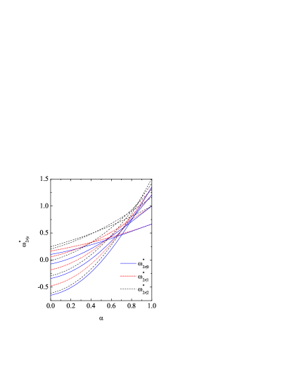
Figure 1: Plot of (from bottom to top at $\alpha=0$) $\omega_{10|0}^{*}$, $\omega_{8|2}^{*}$, $\omega_{8|1}^{*}$, $\omega_{8|0}^{*}$, $\omega_{6|2}^{*}$, $\omega_{6|1}^{*}$, $\omega_{6|0}^{*}$, $\omega_{4|2}^{*}$ $\omega_{4|1}^{*}$, $\omega_{4|0}^{*}$, $\omega_{2|1}*$, $\omega_{2|2}^{*}$, and $\omega_{0|2}^{*}$. The dimensionality is $d=3$.

Figure 1 displays the $\alpha$-dependence of the (scaled) shifted collisional rates $\omega_{2r|s}^{*}\equiv\omega_{2r|s}/\nu_{0}$ with $s=0,1,2$ and $2r+s\leq 10$ for the three-dimensional case ($d=3$). Of course, the null collisional rates $\omega_{0|0}=\omega_{0|1}=\omega_{2|0}=0$ are not plotted. Several comments are in order. Firstly, the degeneracy $\omega_{2r-2|1}=\omega_{2r|0}$ present in the elastic limit S09b ; TM80 is broken, yielding $\omega_{2r-2|1}<\omega_{2r|0}$. Analogously, the linear relationship $d\omega_{2r|1}=(d-1)\omega_{2r-2|2}+\omega_{2r|0}$ for elastic Maxwell particles no longer holds if $\alpha<1$, except in the case $r=1$, where one has $d\omega_{2|1}=(d-1)\omega_{0|2}$ for any $\alpha$ GS07 . Secondly, we observe that all the shifted collisional rates monotonically decrease with increasing dissipation, eventually becoming negative, except those corresponding to $2r+s\leq 5$. The physical implications of this change of sign will be discussed in the next section. A further observation that can be extracted from Fig. 1 is that the impact of $\alpha$ on $\omega_{2r|s}$ becomes generally more pronounced as the degree $2r+s$ increases. In the case of the unshifted collisional rates $\nu_{2r|s}$, a graph similar to Fig. 1 (not reported here) shows a non-monotonic dependence on $\alpha$: they first increase with increasing inelasticity, reach a maximum, and then decrease smoothly. In contrast to the shifted collisional rates $\omega_{2r|s}$, the collisional rates $\nu_{2r|s}$ are always positive, as expected on physical grounds.

4 Diverging moments in the HCS

The Boltzmann equation for the HCS is given by Eq. (1) with $\nabla\to 0$. It is more convenient to rewrite it in terms of the scaled distribution

$$f^{*}(\mathbf{c}(t),t)=\frac{1}{n}[{2T(t)}/{m}]^{d/2}f(\mathbf{v},t),\quad\mathbf{c}(t)={\mathbf{v}}/{\sqrt{2T(t)/m}}.$$ (20)

The resulting Boltzmann equation is

$$\partial_{\tau}f^{*}(\mathbf{c},\tau)+\frac{\nu_{0|2}^{*}}{2}\frac{\partial}{\partial{\mathbf{c}}}\cdot\left[\mathbf{c}f^{*}(\mathbf{c},\tau)\right]=J^{*}[\mathbf{c}|f^{*},f^{*}],$$ (21)

where ${\text{d}}\tau=\nu_{0}{\text{d}}t$, $\nu_{2|0}^{*}\equiv\nu_{2|0}/\nu_{0}$ is the reduced cooling rate, and $J^{*}$ is the dimensionless Boltzmann collision operator. From Eq. (21), and taking into account Eq. (7), one gets the time evolution equation of the moments:

$$\partial_{\tau}M_{2r|\bar{s}}^{*}=-\omega_{2r|s}^{*}M_{2r|\bar{s}}^{*}+\frac{n}{\nu_{0}}\sum_{r^{\prime},r^{\prime\prime},\bar{s}^{\prime},\bar{s}^{\prime\prime}}^{\dagger}\lambda_{r^{\prime}r^{\prime\prime}|\bar{s}^{\prime}\bar{s}^{\prime\prime}\bar{s}}M_{2r^{\prime}|\bar{s}^{\prime}}^{*}M_{2r^{\prime\prime}|\bar{s}^{\prime\prime}}^{*}.$$ (22)

If the distribution function is isotropic, i.e., $f^{*}(\mathbf{c},\tau)=f^{*}(c,\tau)$, then the only non-vanishing moments are $M_{2r|0}^{*}(\tau)$. We will refer to them as the isotropic moments. On the other hand, if the initial distribution function $f^{*}(\mathbf{c},0)$ is not isotropic, the other moments, in particular $M_{2r|i}^{*}(\tau)$ and $M_{2r|ij}^{*}(\tau)$, are not necessarily zero. We will call anisotropic odd moments to $M_{2r|i}^{*}(\tau)$ and anisotropic even moments to $M_{2r|ij}^{*}(\tau)$.

Since the time evolution of the scaled velocity moments in the HCS is governed by the shifted collisional rates $\omega_{2r|s}$, the fact that the latter can become negative (for $\alpha$ smaller than a certain threshold value depending on $r$ and $s$) implies that the associated moments diverge in time.

Among the (scaled) moments $M_{2r|0}^{*}$, $M_{2r|i}^{*}$, and $M_{2r|ij}^{*}$, Fig. 1 shows that the lowest-degree diverging moments are (in the three-dimensional case) the sixth-degree moments $M_{4|ij}^{*}$ and $M_{6|0}^{*}$, which diverge for $\alpha\leq 0.020$ and $\alpha\leq 0.145$, respectively. Moments of higher degree diverge for smaller inelasticities. More specifically, $M_{6|i}^{*}$, $M_{6|ij}^{*}$, $M_{8|0}^{*}$, $M_{8|i}^{*}$, $M_{8|ij}^{*}$, and $M_{10|0}^{*}$ diverge for $\alpha$ smaller than $0.261$, $0.331$, $0.386$, $0.444$, $0.482$, and $0.514$, respectively. In general, the larger the degree the larger the threshold value of the coefficient of restitution below which the moment diverges. Given a degree $2r$, the isotropic moment $M_{2r|0}^{*}$ diverges earlier (i.e., with a larger threshold value $\alpha=\alpha_{2r|0}$) than the anisotropic (even) moment $M_{2r-2|ij}^{*}$. The threshold value of $\alpha_{2r|0}$ can be obtained as the solution of the equation $\omega_{2r|0}=0$. From Eq. (15), this is equivalent to

$$\frac{r}{2d}(1-\alpha^{2})=1-\left(\frac{1+\alpha}{2}\right)^{2r}\frac{(\frac{1}{2})_{r}}{(\frac{d}{2})_{r}}-{}_{2}\!F_{1}\left(-r,\frac{1}{2};\frac{d}{2};z\right).$$ (23)

Given an integer value of $r$, Eq. (23) is an equation of degree $2r$ in $\alpha$.

The Boltzmann equation (21) for the scaled distribution function $f^{*}(\mathbf{c},\tau)$ admits a stationary and isotropic solution $\phi_{\infty}(c)$. This corresponds to a self-similar solution to the original Boltzmann equation where all the velocity and time dependence is encapsulated in the scaled velocity $\mathbf{c}$. About ten years ago, Ernst and Brito EB02a ; EB02b conjectured that the general solution of Eq. (21) asymptotically tends to $\phi_{\infty}(c)$ for long times. Let us loosely express this conjecture as

$$\lim_{\tau\to\infty}f^{*}(\mathbf{c},\tau)=\phi_{\infty}(c),$$ (24)

where the precise meaning of the limit needs to be fixed in a rigorous mathematical sense. The existence of the self-similar solution and the convergence rate for the general approach to this state was first addressed in Ref. BC03 . However, in that work the authors imposed conditions that were proven to be unnecessary in Refs. BCG08 ; BCG09 ; BG06 . More recently, proofs of the strong convergence in Sobolev and $L^{1}$ norms for small CCC09 and finite FPTT10 inelasticity have been published. Those proofs hold for any initial data (probability densities with bounded second-degree moments), regardless of being isotropic or not, but they do not imply that any moment of degree higher than two converges to the corresponding moment of the self-similar solution. This stronger moment-to-moment interpretation of the Ernst–Brito conjecture would read

$${\lim_{\tau\to\infty}M_{2r|\bar{s}}^{*}(\tau)=\int{\text{d}}\mathbf{c}\,Y_{2r|\bar{s}}(\mathbf{c})\phi_{\infty}(c).}$$ (25)

As discussed below, this stronger notion of the convergence statement (24) does not hold.

Although the explicit form of $\phi_{\infty}(c)$ is not known, except in the one-dimensional case BMP02 , it is known that it possesses an algebraic high-velocity tail of the form $\phi_{\infty}(\mathbf{c})\sim c^{-d-\gamma_{0}(\alpha)}$, where $\gamma_{0}(\alpha)$ obeys a transcendental equation BK02 ; BCG08 ; BCG09 ; EB02a ; EB02b ; KB02 . As a consequence, the isotropic moments $M_{2r|0}^{*}$ with $2r\geq\gamma_{0}(\alpha)$ diverge. According to the strong convergence property (25), this would imply that, if $M_{2r|0}^{*}(0)=\text{finite}$, then $\lim_{\tau\to\infty}M_{2r|0}^{*}(\tau)=\infty$ if $2r\geq\gamma_{0}(\alpha)$. This is fully consistent with the fact that $\omega_{2r|0}<0$, so that $M_{2r|0}^{*}(\tau)$ indeed diverges in time if $\alpha<\alpha_{2r|0}$. In fact, formally setting $2r=\gamma_{0}$ in Eq. (23) one recovers the transcendental equation for $\gamma_{0}$ derived by an independent method BK02 ; EB02a ; EB02b ; KB02 .

The interesting point is that, as shown above, the anisotropic moments $M_{2r|i}^{*}$ and $M_{2r|ij}^{*}$ can also diverge, unless they are zero in the initial state. The possibility that $\lim_{\tau\to\infty}M_{2r|i}^{*}(\tau)=\infty$ and $\lim_{\tau\to\infty}M_{2r|ij}^{*}(\tau)=\infty$ contradicts the strict moment-to-moment limit (25), since all the anisotropic moments of $\phi_{\infty}(c)$ vanish. Let us elaborate this result in more detail.

In principle, we have derived Eqs. (15)–(17) for $r=\text{integer}$. However, since the hypergeometric function and the Pochhammer symbols are well defined for $r\neq\text{integer}$, we speculate that an analytic continuation of Eqs. (15)–(17) to $r\neq\text{integer}$ is possible. It is then tempting to interpret $\omega_{k|0}^{*}$, $\omega_{k-1|1}^{*}$, and $\omega_{k-2|2}^{*}$ as the quantities governing the asymptotic time evolution of the averages $M_{k|0}^{*}\equiv\langle c^{k}\rangle$, $M_{k-1|i}^{*}\equiv\langle c^{k-1}c_{i}\rangle$, and $M_{k-2|ij}^{*}\equiv\langle c^{k-2}\left(c_{i}c_{j}-d^{-1}c^{2}\delta_{ij}\right)\rangle$, respectively, even if $k/2\neq\text{integer}$ and $(k-1)/2\neq\text{integer}$, although a formal proof of this expectation is beyond the scope of this paper. As said before, $M_{k|0}^{*}\to\infty$ if $k>\gamma_{0}(\alpha)$, where $\omega_{\gamma_{0}|0}^{*}=0$. Analogously, we can expect that the anisotropic quantities $M_{k-1|i}^{*}$ and $M_{k-2|ij}^{*}$ diverge if $k>\gamma_{1}(\alpha)$ and $k>\gamma_{2}(\alpha)$, respectively, where $\gamma_{1}$ and $\gamma_{2}$ are the solutions to the equations $\omega_{\gamma_{1}-1|1}^{*}=0$ and $\omega_{\gamma_{2}-2|2}^{*}=0$.

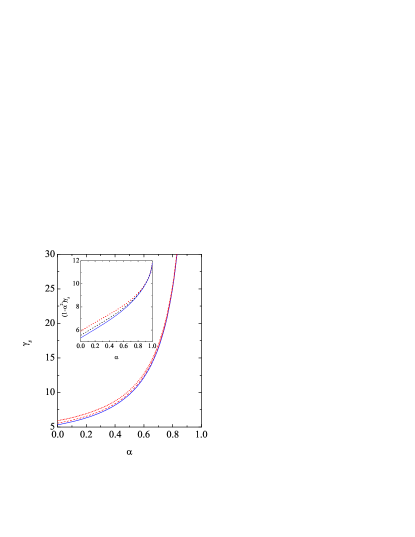
Figure 2: Plot of (from bottom to top) $\gamma_{0}(\alpha)$, $\gamma_{1}(\alpha)$, and $\gamma_{2}(\alpha)$. The inset shows $(1-\alpha^{2})\gamma_{s}$ versus $\alpha$. The dimensionality is $d=3$.

The functions $\gamma_{0}(\alpha)$, $\gamma_{1}(\alpha)$, and $\gamma_{2}(\alpha)$ are displayed in Fig. 2 for $d=3$. In the elastic limit $\alpha\to 1$, the three exponents diverge as $\gamma_{s}\approx 4d/(1-\alpha^{2})$ BK02 ; KB02 , as shown in the inset of Fig. 2. We observe that $\gamma_{0}(\alpha)<\gamma_{1}(\alpha)<\gamma_{2}(\alpha)$. This implies that, at a given value of $\alpha$ the isotropic average $M_{k|0}^{*}$ starts to diverge before the anisotropic (odd) average $M_{k-1|i}^{*}$ does, and the latter does it before the anisotropic (even) average $M_{k-2|ij}^{*}$ does. Stated differently, if we focus on the ratios between the anisotropic and the isotropic averages, we can expect the asymptotic behaviors

$$\frac{M_{k-1|i}^{*}}{M_{k|0}^{*}}\sim e^{-(\omega_{k-1|1}^{*}-\omega_{k|0}^{*})\tau},\quad\frac{M_{k-2|ij}^{*}}{M_{k|0}^{*}}\sim e^{-(\omega_{k-2|2}^{*}-\omega_{k|0}^{*})\tau}.$$ (26)

Since $\omega_{k-2|2}^{*}>\omega_{k-1|1}^{*}>\omega_{k|0}^{*}$, it turns out that

$$\lim_{\tau\to\infty}\frac{M_{k-1|i}^{*}}{M_{k|0}^{*}}=0,\quad\lim_{\tau\to\infty}\frac{M_{k-2|ij}^{*}}{M_{k|0}^{*}}=0.$$ (27)

Therefore, the anisotropic moments, relative to the isotropic moments of the same degree, asymptotically go to zero (the anisotropic even moments more rapidly than the anisotropic odd ones). From that point of view, Eq. (27) can be seen as a weak validation of a moment-to-moment interpretation of Eq. (24) for initial anisotropic distributions.

The one-dimensional system deserves some separate comments. In that case, the self-similar solution is $\phi_{\infty}(c)=(2^{3/2}/\pi)(1+2c^{2})^{-2}$ BMP02 , so that $\gamma_{0}=3$ and the moments $\langle c^{k}\rangle$ with $k\geq 3$ diverge. This agrees with Eq. (18), according to which $\omega_{k|0}^{*}\leq 0$ for $k\geq 3$. Analogously, from Eq. (19) one gets $\gamma_{1}=3$. In particular, the isotropic moment $\langle c^{3}\rangle$ diverges, while the anisotropic moment $\langle c^{2}c_{x}\rangle$ (proportional to the heat flux) keeps its initial value BK00 ; GS07 . Therefore, $\langle c^{2}c_{x}\rangle/\langle c^{3}\rangle\to 0$. On the other hand, since $\omega_{k|0}^{*}=\omega_{k-1|1}^{*}<0$ for $k>3$, there exist two possible scenarios for the ratios $\langle c^{k-1}c_{x}\rangle/\langle c^{k}\rangle$: either they tend to constant values or they decay more slowly than exponentially. A deeper investigation is needed to elucidate between these two possibilities.

5 Conclusion

To summarize, we have shown that the strong notion (25) of the Ernst–Brito conjecture cannot be strictly true since it does not hold for anisotropic initial conditions. However, we conjecture that $M^{*}_{2r|\bar{s}}(\tau)/M^{*}_{2r+s|0}(\tau)\to 0$ when $\bar{s}\neq 0$, even if $M^{*}_{2r|\bar{s}}(\tau)\to\infty$, as shown by Eq. (27) for $\bar{s}=i$ ($s=1$) and $\bar{s}=ij$ ($s=2$). In order to elaborate further this conjecture, let us decompose $f^{*}(\mathbf{c},\tau)$ into its isotropic, anisotropic symmetric, and antisymmetric parts:

$$f^{*}(\mathbf{c},\tau)=\phi(c,\tau)+\widetilde{f}_{+}^{*}(\mathbf{c},\tau)+f_{-}^{*}(\mathbf{c},\tau),\quad$$ (28)

where

$$\widetilde{f}_{+}^{*}(\mathbf{c},\tau)\equiv f_{+}^{*}(\mathbf{c},\tau)-\phi({c},\tau),\quad\phi({c},\tau)\equiv\frac{1}{\Omega_{d}}\int{\text{d}}\widehat{\mathbf{c}}\,f_{+}(\mathbf{c},\tau),$$ (29)

$$f_{\pm}^{*}(\mathbf{c},\tau)\equiv\frac{1}{2}\left[f^{*}(\mathbf{c},\tau)\pm f^{*}(-\mathbf{c},\tau)\right].$$ (30)

As a consequence, the velocity moments $M_{k|0}^{*}(\tau)$, $M_{k-1|i}^{*}(\tau)$, and $M_{k-2|ij}^{*}(\tau)$ are related to $\phi(c,\tau)$, ${f}_{-}^{*}(\mathbf{c},\tau)$, and $\widetilde{f}_{+}^{*}(\mathbf{c},\tau)$, respectively. If the “sizes” of these three contributions are measured through those three classes of moments, we can say that, as time progresses, the two anisotropic parts of $f^{*}$ become negligible versus the isotropic part, i.e., $|f_{-}^{*}(\mathbf{c},\tau)|\ll\phi({c},\tau)$ and $|\widetilde{f}_{+}^{*}(\mathbf{c},\tau)|\ll\phi({c},\tau)$, in the sense of Eq. (27). Moreover, $\lim_{\tau\to\infty}\phi(c)=\phi_{\infty}(c)$. We further speculate that the high-velocity tails of the anisotropic contributions tend to the forms

$$f_{-}^{*}(\mathbf{c},\tau)\to\chi_{-}(\widehat{\mathbf{c}})c^{-d-\gamma_{1}(\alpha)},\quad\widetilde{f}_{+}^{*}(\mathbf{c},\tau)\to\widetilde{\chi}_{+}(\widehat{\mathbf{c}})c^{-d-\gamma_{2}(\alpha)},$$ (31)

where the angular functions $\chi_{-}(\widehat{\mathbf{c}})$ and $\widetilde{\chi}_{+}(\widehat{\mathbf{c}})$ depend on the initial conditions. A confirmation of the above expectations requires a more refined analysis.

- (1) Abramowitz, M., Stegun, I.A. (eds.): Handbook of Mathematical Functions. Dover, New York (1972)
- (2) Baldassarri, A., Marini Bettolo Marconi, U., Puglisi, A.: Influence of correlations on the velocity statistics of scalar granular gases. Europhys. Lett. 58, 14–20 (2002)
- (3) Ben-Naim, E., Krapivsky, P.L.: Multiscaling in inelastic collisions. Phys. Rev. E 61, R5–R8 (2000)
- (4) Ben-Naim, E., Krapivsky, P.L.: Scaling, multiscaling, and nontrivial exponents in inelastic collision processes. Phys. Rev. E 66, 011,309 (2002)
- (5) Ben-Naim, E., Krapivsky, P.L.: The inelastic Maxwell model. In: T. Pöschel, S. Luding (eds.) Granular Gas Dynamics, Lecture Notes in Physics, vol. 624, pp. 65–94. Springer, Berlin, Germany (2003)
- (6) Bisi, M., Carrillo, J.A., Toscani, G.: Decay rates in probability metrics towards homogeneous cooling states for the inelastic Maxwell model. J. Stat. Phys. 124, 625–653 (2006)
- (7) Bobylev, A.V., Carrillo, J.A., Gamba, I.M.: On some properties of kinetic and hydrodynamic equations for inelastic interactions. J. Stat. Phys. 98, 743–773 (2000)
- (8) Bobylev, A.V., Cercignani, C.: Self-similar asymptotics for the Boltzmann equation with inelastic and elastic interactions. J. Stat. Phys. 110, 333–375 (2003)
- (9) Bobylev, A.V., Cercignani, C., Gamba, I.M.: Generalized kinetic Maxwell models of granular gases, Lecture Notes in Mathematics, vol. 1937, pp. 23–58. Springer, Berlin (2008)
- (10) Bobylev, A.V., Cercignani, C., Gamba, I.M.: On the self-similar asymptotics for generalized non-linear kinetic Maxwell models. Commun. Math. Phys. 291, 599–644 (2009)
- (11) Bobylev, A.V., Cercignani, C., Toscani, G.: Proof of an asymptotic property of self-similar solutions of the Boltzmann equation for granular materials. J. Stat. Phys. 111, 403–417 (2003)
- (12) Bobylev, A.V., Gamba, I.M.: Boltzmann equations for mixtures of Maxwell gases: exact solutions and power like tails. J. Stat. Phys. 124, 497–516 (2006)
- (13) Bolley, F., Carrillo, J.A.: Tanaka theorem for inelastic Maxwell models. Commun. Math. Phys. 276, 287–314 (2007)
- (14) Brey, J.J., García de Soria, M.I., Maynar, P.: Breakdown of hydrodynamics in the inelastic Maxwell model of granular gases. Phys. Rev. E 82, 021,303 (2010)
- (15) Brilliantov, N.V., Pöschel, T.: Kinetic Theory of Granular Gases. Oxford University Press, Oxford (2004)
- (16) Brito, R., Ernst, M.H.: Anomalous velocity distributions in inelastic Maxwell gases. In: E. Korutcheva, R. Cuerno (eds.) Advances in Condensed Matter and Statistical Mechanics, pp. 177–202. Nova Science Publishers, New York, USA (2004)
- (17) Carlen, E.A., Carrillo, J.A., Carvalho, M.C.: Strong convergence towards homogeneous cooling states for dissipative Maxwell models. Ann. I. H. Poincaré – AN 26, 167–1700 (2009)
- (18) Carrillo, J.A., Cercignani, C., Gamba, I.M.: Steady states of a Boltzmann equation for driven granular media. Phys. Rev. E 62, 7700–7707 (2000)
- (19) Carrillo, J.A., Toscani, G.: Contractive probability metrics and asymptotic behavior of dissipative kinetic equations. Riv. Mat. Univ. Parma 6, 75–198 (2007)
- (20) Ernst, M.H.: Exact solutions of the nonlinear Boltzmann equation. Phys. Rep. 78, 1–171 (1981)
- (21) Ernst, M.H., Brito, R.: High-energy tails for inelastic Maxwell models. Europhys. Lett. 58, 182–187 (2002)
- (22) Ernst, M.H., Brito, R.: Scaling solutions of inelastic Boltzmann equations with over-populated high energy tails. J. Stat. Phys. 109, 407–432 (2002)
- (23) Furioli, G., Pulvirenti, A., Terraneo, E., Toscani, G.: Convergence to self-similarity for the Boltzmann equation for strongly inelastic Maxwell molecules. Ann. I. H. Poincaré – AN 27, 719–737 (2010)
- (24) Garzó, V., Santos, A.: Third and fourth degree collisional moments for inelastic Maxwell model. J. Phys. A: Math. Theor. 40, 14,927–14,943 (2007)
- (25) Garzó, V., Santos, A.: Hydrodynamics of inelastic Maxwell models. Math. Model. Nat. Phenom. 6(4), 37–76 (2011)
- (26) Krapivsky, P.L., Ben-Naim, E.: Nontrivial velocity distributions in inelastic gases. J. Phys. A: Math. Gen. 35, L147–L152 (2002)
- (27) Santos, A.: Transport coefficients of -dimensional inelastic Maxwell models. Physica A 321, 442–466 (2003)
- (28) Santos, A.: Solutions of the moment hierarchy in the kinetic theory of Maxwell models. Cont. Mech. Thermodyn. 21, 361–387 (2009)
- (29) Truesdell, C., Muncaster, R.G.: Fundamentals of Maxwell’s Kinetic Theory of a Simple Monatomic Gas. Academic Press, New York (1980)