Quasiparticle Renormalization and Pairing Correlations in Spherical Superfluid Nuclei

Abstract

We present a detailed discussion of the solution of Nambu-Gor’kov equations in superfluid nuclei, which provide a consistent framework to deal with the interplay between particle-hole and particle-particle channel, including the effects of the fragmentation of the quasiparticle strength and of the pairing interaction induced by the exchange of collective vibrations. The coupling between quasiparticle and vibrations is determined from the experimental polarizability of the low-lying collective surface vibrations. This coupling is used to renormalize the properties of quasiparticles obtained from a BCS calculation using the bare nucleon-nucleon interaction. We apply the formalism to the case of the nucleus ¹²⁰Sn, showing results for the low-energy spectrum and the quasiparticle strength distribution in neighbouring odd nuclei and for the neutron pairing gap.

I Introduction

The key role played by pairing correlations in atomic nuclei was recognized soon after the development of BCS theory. The number of Cooper pairs involved is small, and one can study nuclear superfluidity within BCS in terms of specific orbitals lying close to the Fermi energy, interacting through an attractive nucleon-nucleon force. However, the properties of the particles are considerably renormalized by the coupling to the collective vibration of the system, which leads to an enhancement of the effective mass and of the level density close to the Fermi energy, and to a fragmentation of the particle strength observed in one-nucleon transfer reactions. While these phenomena have been extensively studied in normal nuclei mah:85 ; soloviev , their consequences on pairing correlations have been much less investigated. Obtaining an accurate description of these effects requires to go beyond the BCS framework. A convenient formalism that allows one to consider the interplay between the particle-hole and the particle-particle channel is offered by the Nambu-Gor’kov equations, used in condensed matter to deal with strong coupling superconductivity gorkov ; nambu ; eliashberg . These equations imply the calculation of energy-dependent normal and abnormal self-energies, take into account the pairing interaction induced by the exchange of collective vibrations between members of the Cooper pairs and lead to theoretical predictions concerning the low-energy part of the nuclear spectrum; they also produce the structure elements needed for a consistent calculation of one- and two-nucleon transfer reactions gregory .

In this paper we extend our previous investigations concerning the microscopic origin of pairing (cf. in particular prl_noi -pastore:08 ). In Section II we provide a detailed account of the formalism, comparing two different schemes for the dealing with the Nambu-Gor’kov equations, either solving first the BCS equations with the bare nucleon-nucleon force and then adding renormalization effects (prior scheme, cf. Section II.1) , or dealing at the same time with both sources of pairing (post scheme, cf. Section II.2). The coupling between quasiparticle and vibrations is computed according to the basic rules of Nuclear Field Theory (NFT) nft1 ; nft2 ; BM:75 . Use is made of the collective model of Bohr and Mottelson to calculate the properties of vibrational states in the Quasiparticle Random Phase Approximation (QRPA) with a separable force, with a coupling constant chosen so as to reproduce the experimental properties of low-lying collective surface modes. In this way we avoid the use of free parameters in the calculation, which then only depends on the choice of the interaction adopted to produce the mean field. In most of the computations we shall use the SLy4 effective interaction, which provides a good reproduction of the overall mean field properties, and leads to a reasonable level density around the Fermi energy, after including renormalization effects. We shall derive gap equations which generalize the usual BCS expression, lend themselves to useful approximations and allow one to make contact with other studies. In Section III we shall solve the Nambu-Gor’kov equations in the case of ¹²⁰Sn, comparing the theoretical low-lying spectrum in neighbouring odd nuclei with experimental data derived from one-neutron transfer reactions. We shall also compare the results obtained with a self-consistent iterative solution of the Nambu-Gor’kov equations with the quasiparticle approximation. It is possible to clearly separate the contributions to the pairing gap associated with the bare nucleon-nucleon force and with the renormalization effects. We find that the two contributions have comparable magnitudes, confirming previous studies. We shall also briefly consider the role played by spin modes, which provide a repulsive contribution to pairing in the ${}^{1}S_{0}$ channel, whose magnitude is however very uncertain. Conclusions and a hindsight will be presented in Section IV. The sensitivity of our results to various elements of the calculations is discussed in the Appendix.

II The formalism

The object of our study are pairing correlations in superfluid nuclei taking into account both the contribution of the bare nucleon-nucleon interaction, and the many-body effects associated with the coupling between particles and vibrations (cf. Fig. 1).

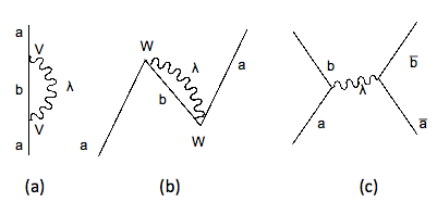
Figure 1: Basic diagrams taken into account in the present study, which renormalize the normal and abnormal self-energies obtained in mean field calculations: polarization (a), correlation (b), induced pairing interaction (c) processes.

Our approach will be based on two basic assumptions:

(A) We shall start from a mean field obtained with a Hartree-Fock (HF) calculation with an effective force. Our quantitative results will then depend to some extent on the choice of the force adopted to produce the mean field, because pairing correlations are very sensitive to the position of the single-particle levels. In principle, one could aim at determining the parameters of a new effective force, by comparing the results obtained including renormalization with experimental data. This would require an extensive investigation, considering several isotopic chains. In this work we shall limit ourselves to the study of renormalization effects in the single nucleus ¹²⁰Sn, adopting existing effective forces which lead to a reasonable description of the available data - although we are aware that the quantitative aspects of our findings might be improved by a more careful determination of the mean field.

(B) We shall not consider explicitly the renormalization processes affecting the vibrations of the system epj:04 ; bort:80 ; broglia:03 . The main diagrams renormalizing the energy of the phonons are shown in Fig. 2(b1) (self-energy correction renormalizing the energy of the particle-hole transitions) and Fig. 2(b2) (vertex correction renormalizing the particle-hole interaction), while the diagrams shown in Fig. 2(d1) and Fig. 2(d2) renormalize the transition strength. The explicit inclusion of renormalization effects on phonons, on par with those on single-particle levels, represents an ambitious program that has been attempted only in a few cases for closed-shell nuclei dickhoff1 ; dickhoff2 ; barbieri . We shall instead take the view that such renormalization effects, if taken properly into account, should lead to agreement with experiment. In particular, we shall take the transition densities which are at the basis of the interweaving of single-particle (quasiparticle) degrees of freedom and collective modes from the collective macroscopic Bohr-Mottelson model. We shall determine the Particle-Vibration Coupling (PVC) strength (cf. Fig. 2(b2)) from a QRPA calculation tuned to reproduce the experimental properties of the low-lying phonons, using a mean field with an effective mass $m^{*}=m$ that reproduces the experimental single-particle level density (cf. Fig. 2(b1)) (see Section III for more details).

Within this frozen-phonon approximation, as a possible alternative, one might calculate the PVC microscopically making use of the transition density of the RPA phonons obtained from a self-consistent calculation performed with the same effective force employed to obtain the HF mean field. Calculations of this kind have been performed several times in the past for non-superfluid nuclei, with various degree of approximations mah:85 ; see colo for a recent calculation aiming at a complete self-consistence. The main drawback in this approach lies in the fact that QRPA leads to a relatively poor reproduction of the experimental energy and of the transition strength of the low-lying collective vibrational states in semimagic nuclei (for recent QRPA calculations cf. e.g. ansari:06 ,tera:08 ), which provide the main contribution to renormalization effects. This is consistent with the fact that processes beyond QRPA can strongly renomalize the phonon properties. We shall instead take the view that renormalization effects, if taken properly into account beyond the frozen phonon approximation, should lead to agreement with experiment. As a consequence, we shall take the PVC from a QRPA calculation tuned to reproduce the experimental properties of the low-lying phonons, using a mean field with an effective mass $m^{*}=m$ that reproduces the experimental level density. In other words, we shall assume that vertex corrections are effectively included in our PVC.

Figure 2: The self-energy (a) of the vibrations calculated in the QRPA approximation is renormalized by the basic diagrams (b1) (leading to a renormalization of the particle-hole energies) and (b2) (vertex correction renormalizing the particle-hole interaction). Similarly, the QRPA transition strength (c) is renormalized by the corresponding diagrams (d1) and (d2).

The actual implementation of assumptions (A) and (B) will be presented below in the next Sections. Other, less essential assumptions will be adopted in our calculation in order to reduce the computational complexity. First of all, we shall limit the investigation of renormalization processes to states lying close to the Fermi energy. We shall then take into account the fact that the bare interaction - even considering its soft-core or $V_{{\rm low}k}$ versions - couples the single-particle states lying close to the Fermi energy with states lying up to several hundreds of MeV, while the phonon-mediated pairing interaction acts between pair of states separated by a few MeV noi_schuck ; dick:book . This suggests the convenience of a separate treatment of the two interactions in the pairing problem, by performing a HF+BCS calculation prior to the calculation of many-body effects. We shall refer to this approach as the ${\it prior\;scheme}$. Otherwise, one is forced to consider the bare and the induced interaction on the same footing (${\it post\;scheme}$). In the following we shall first illustrate in detail the prior scheme, which will be used in most calculations presented in this paper. We shall then outline the main modifications involved in the post scheme.

II.1 The prior scheme

A convenient formalism for the calculation of the properties of quasiparticles in superfluid nuclei within the prior scheme was given by Van der Sluys et al. Sluys:93 , although they did not devote particular attention to the renormalization of pairing correlations. In this approach one first accounts for the action of the bare force with a HF+BCS calculation, discussed in more detail in Section III.1.1 , leading to quasiparticle energies $E_{a}$, quasiparticles amplitudes $u_{a}$ and $v_{a}$ and to a pairing gap $\Delta^{BCS}_{a}$. One then renormalizes the obtained quasiparticles including the coupling to vibrations calculated in the QRPA. The derivation of the formalism was based on the equation of motion method, which has a very close relation to the Green’s functions formalism used to derive the Nambu-Gor’kov equations, commonly used to study superconductivity in condensed matter physics Schr:64 .

In order to calculate the renormalization of a quasiparticle in spherical nuclei, denoted by its associated quantum numbers $a\equiv\{nlj\}$, one has to solve a system of linear equations obtained coupling the quasiparticle with more complex configurations including phonon states through the basic vertices $V$ and $W$ shown in Fig. 1. The phonons are characterized by their angular momentum $\lambda$ and by their energy $\hbar\omega_{\lambda,\nu}$. We shall assume that phonons have natural parity, $\pi=(-1)^{\lambda}$ (see however Section III.1.3). For illustration, we write the diagonalization problem including only two other quasiparticle states $b$ and $c$, and a single phonon ${\lambda,\nu}$:

$$\left(\matrix{E_{a}&V(ab\lambda\nu)&V(ac\lambda\nu)&W(ab\lambda\nu)&W(ac\lambda\nu)&0\cr V(ab\lambda\nu)&\hbar\omega_{\lambda\nu}+E_{b}&0&0&0&W(ab\lambda\nu)\cr V(ac\lambda\nu)&0&\hbar\omega_{\lambda\nu}+E_{c}&0&0&W(ac\lambda\nu)\cr W(ab\lambda\nu)&0&0&-\hbar\omega_{\lambda\nu}-E_{b}&0&-V(ab\lambda\nu)\cr W(ac\lambda\nu)&0&0&0&-\hbar\omega_{\lambda\nu}-E_{c}&-V(ac\lambda\nu)\cr 0&W(ab\lambda\nu)&W(ac\lambda\nu)&-V(ab\lambda\nu)&-V(ac\lambda\nu)&-E_{a}}\right)\left(\matrix{x_{a(n)}\cr C_{a(n),b,\lambda\nu}\cr C_{a(n),c,\lambda\nu}\cr-D_{a(n),b,\lambda\nu}\cr-D_{a(n),c,\lambda\nu}\cr-y_{a(n)}}\right)=$$

$$\tilde{E}_{a(n)}\left(\matrix{x_{a(n)}\cr C_{a(n),b,\lambda\nu}\cr C_{a(n),c,\lambda\nu}\cr-D_{a(n),b,\lambda\nu}\cr-D_{a(n),c,\lambda\nu}\cr-y_{a(n)}}\right)$$ (1)

Many eigenvalues $\tilde{E}_{a(n)}$ and eigenstates $a(n)$ are obtained from the diagonalization of the matrix (1), giving rise to a fragmentation of the associated quasiparticle strength. For a given eigenvalue $\tilde{E}_{a(n)}>0$ there exists a corresponding eigenvalue $\tilde{E}_{a(-n)}=-\tilde{E}_{a(n)}$. As in standard BCS theory, we will keep only positive energy solutions, $n>0$.

The amplitudes obey the normalization condition

$$x_{a(n)}^{2}+\sum_{b,\lambda,\nu}\left[C_{a(n),b,\lambda\nu}^{2}\right]+y_{a(n)}^{2}+\sum_{b,\lambda,\nu}\left[D_{a(n),b,\lambda\nu}^{2}\right]=1,$$ (2)

$C_{a(n),b,\lambda\nu}$ and $D_{a(n),b,\lambda\nu}$ being the components on the complex $1qp\otimes 1ph$ states, while $x_{a(n)}$ and $y_{a(n)}$ are the components on the original $1qp$ state $a$. The fragment $a(n)$ carries a fraction of the strength

$$N_{a(n)}=x_{a(n)}^{2}+y_{a(n)}^{2}<1$$ (3)

which is to be compared with the experimental quasiparticle strength, as determined for example in one-particle-transfer reactions.

The excitation operator appearing in Eq.(1)

$$\tilde{O}^{\dagger}_{a(n)}=\tilde{\alpha}^{\dagger}_{a(n)_{qp}}+C_{a(n)b\lambda\nu}\alpha^{\dagger}_{b}\Gamma^{\dagger}_{\lambda\nu}-D_{a(n)b\lambda\nu}\alpha_{\bar{b}}\Gamma_{\lambda\bar{\nu}}$$

contains the quasiparticle component

$$\tilde{\alpha}^{\dagger}_{a(n)_{qp}}=x_{a(n)}\alpha^{\dagger}_{a}-y_{a(n)}\alpha_{\bar{a}}.$$

Taking into account the BCS Bogoliubov transformation,

$$\alpha^{\dagger}_{a}=u_{a}a^{\dagger}_{a}+v_{a}a_{\bar{a}}$$

one can write

$$\tilde{\alpha}^{\dagger}_{a(n)_{qp}}=\tilde{u}_{a(n)}a^{\dagger}_{a}+\tilde{v}_{a(n)}a_{\bar{a}},$$

where the quantities

$$\tilde{u}_{a(n)}=x_{a(n)}u_{a}-y_{a(n)}v_{a}$$ (4)

$$\tilde{v}_{a(n)}=x_{a(n)}v_{a}+y_{a(n)}u_{a}.$$ (5)

represent the new quasiparticle amplitudes associated with a given fragment $a(n)$: their squares give the spectroscopic factors associated with one-nucleon transfer reactions.

We can then calculate the renormalized pairing gap as (cf. below Eq. (54))

$$\tilde{\Delta}_{a(n)}=\frac{2\tilde{E}_{a(n)}\tilde{u}_{a(n)}\tilde{v}_{a(n)}}{\tilde{u}_{a(n)}^{2}+\tilde{v}_{a(n)}^{2}}.$$ (6)

The quasiparticle-phonon matrix elements $V(ab\lambda\nu)$ and $W(ab\lambda\nu)$ in Eq. (1) are given by

$$V(ab\lambda\nu)=\left[\frac{2\lambda+1}{2j_{a}+1}\right]^{1/2}\sum_{c\leq d}(1+\delta_{cd})^{-1/2}\times$$ (7)

$$\left[X_{cd}(\lambda\nu)V(cd\lambda b;a)+(-1)^{j_{a}-j_{b}+\lambda}Y_{cd}(\lambda\nu)V(cd\lambda a;b)\right]$$ (8)

and

$$W(ab\lambda\nu)=\left[\frac{2\lambda+1}{2j_{a}+1}\right]^{1/2}\sum_{c\leq d}(1+\delta_{cd})^{-1/2}\times$$ (9)

$$\left[X_{cd}(\lambda\nu)R(cd\lambda b;a)+(-1)^{j_{a}-j_{b}+\lambda}Y_{cd}(\lambda\nu)Q(cd\lambda a;b)\right],$$ (10)

where $X_{cd}$ and $Y_{cd}$ are the forward and backward amplitudes resulting from the QRPA calculation.

The terms $V(cd\lambda b;a)$, $Q(cd\lambda b;a)$ and $R(cd\lambda b;a)$ are given by

$$V(cd\lambda b;a)=-(u_{a}v_{b}u_{c}u_{d}-v_{a}u_{b}v_{c}v_{d})G(abcd\lambda)$$ (11)

$$+(u_{a}u_{b}u_{c}v_{d}-v_{a}v_{b}v_{c}u_{d})F(abcd\lambda)$$ (12)

$$+(-1)^{j_{c}-j_{d}+\lambda}(u_{a}u_{b}v_{c}u_{d}-v_{a}v_{b}u_{c}v_{d})F(abdc\lambda)$$ (13)

$$Q(cd\lambda b;a)=(u_{a}u_{b}u_{c}u_{d}+v_{a}v_{b}v_{c}v_{d})G(abcd\lambda)$$ (14)

$$+(u_{a}v_{b}u_{c}v_{d}+v_{a}u_{b}v_{c}v_{d})F(abcd\lambda)$$ (15)

$$+(-1)^{j_{c}-j_{d}+\lambda}(u_{a}v_{b}v_{c}u_{d}+v_{a}u_{b}v_{c}u_{d})F(abdc\lambda)$$ (16)

$$R(cd\lambda b;a)=-(u_{a}u_{b}v_{c}v_{d}+v_{a}v_{b}u_{c}u_{d})G(abcd\lambda)$$ (17)

$$+(u_{a}v_{b}v_{c}u_{d}+v_{a}u_{b}u_{c}v_{d})F(abcd\lambda)$$ (18)

$$+(-1)^{j_{c}-j_{d}+\lambda}(u_{a}v_{b}u_{c}u_{d}+v_{a}u_{b}v_{c}v_{d})F(abdc\lambda),$$ (19)

where $F(abcd\lambda)$ and $G(abcd\lambda)$ denote the angular momentum coupled antisymmetrized particle-hole and particle-particle $<ab\lambda|V|cd\lambda>_{as}$ matrix element respectively. Note that in the limit of non-superfluid nuclei (all $u,v$ terms equal to 0 or 1), the matrix elements $V(ab\lambda\nu)$ connect pairs of states $a,b$ above or below the Fermi energy through the $F-$terms, and pairs of states on opposite parts of the Fermi energy through the $G-$terms; while the opposite is true for the $W(ab\lambda\nu)$ matrix elements. In the following we shall not take into account the coupling with pair vibration modes, neglecting the $G$ terms in Eqs. (13)-(19). While this coupling is known to be relevant for closed shell nuclei, it is expected to be much less important for the superfluid case, since most of the two-particle transfer strength is already incorporated in the BCS ground state (gauge space deformed) wave function broglia:advances .

The QRPA amplitudes could be obtained from a calculation performed using the same force adopted in the HF+BCS calculations. In our approach, the QRPA calculation is instead decoupled from the renormalization process, in keeping with the main assumption (B) discussed above. In our QRPA calculation we shall use the separable force

$$V(\vec{r}_{1},\vec{r}_{2})=-\kappa_{self}\;r_{1}\frac{\partial U}{\partial r_{1}}r_{2}\frac{\partial U}{\partial r_{2}}\sum_{\lambda\mu}\chi_{\lambda}Y^{*}_{\lambda\mu}(\theta_{1})Y_{\lambda\mu}(\theta_{2})$$ (20)

where $U(r)$ is a potential that gives a good reproduction of the experimental levels. In practice, we adopt the Woods-Saxon parametrization given in BM:69 (cf. Eq. (2-182)) together with an empirical pairing coupling constant adjusted to reproduce the pairing gap deduced from the experimental odd-even mass difference. The parameters $\chi_{\lambda}$ are determined so as to get a good agreement with the observed properties (energy and transition strength) of the low-lying surface modes. More precisely, we shall reproduce the polarizability $\beta^{2}_{\lambda 1}/\hbar\omega_{\lambda 1}$ of the low-lying modes, where $\beta_{\lambda\nu}$ denotes the experimental nuclear deformation parameter. In fact, the matrix elements of the phonon-induced pairing interaction for levels close to the Fermi energy are approximately proportional to the polarizability of the mode (cf. Eq. (46) below). The resulting values of $\chi_{\lambda}$ turn out to be close to 1 (cf. Section III), indicating that the QRPA coupling constant is close to the Bohr-Mottelson self-consistent coupling constant $\kappa_{self}=\left[{\int r\frac{\partial\rho}{\partial r}r\frac{\partial U}{\partial r}r^{2}dr}\right]^{-1}$.

This scheme then reduces to the collective particle-shape vibration (phonon) coupling scheme given by Bohr and Mottelson BM:75 (cf. Eqs. 6-207- 6-209). In fact the particle-hole matrix elements, neglecting the exchange terms (cf. on this point rowe , Eq. (14.54) and Chap.16), are given by

$$F(abcd\lambda)=-\kappa_{self}\chi_{\lambda}<ab\lambda\mu|r_{1}\frac{\partial U}{\partial r_{1}}Y^{*}_{\lambda\mu}(\theta_{1})|0><0|r_{2}\frac{\partial U}{\partial r_{2}}Y^{*}_{\lambda\mu}(\theta_{2})|cd\lambda\mu>$$ (21)

where $\mu$ is any of the $z$-projections of the angular momentum $\lambda$. In this expression the QRPA-like single-particle indices $(c,d)$ and the scattered particle indices $(a,b)$ appear in separated factors, so that one gets the angular momentum reordering property $F(abdc\lambda)=(-1)^{j_{c}-j_{d}+\lambda}F(abcd\lambda)=(-1)^{j_{a}-j_{b}+\lambda}F(bacd\lambda)$, and

$$V(ab\lambda\nu)=-\kappa_{self}\chi_{\lambda}(u_{a}u_{b}-v_{a}v_{b})<ab\lambda\mu|r_{1}\frac{\partial U}{\partial r_{1}}Y^{*}_{\lambda\mu}(\theta_{1})|0>\left[\frac{2\lambda+1}{2j_{a}+1}\right]^{1/2}$$ (22)

$$\times\sum_{c\leq d}(1+\delta_{cd})^{-1/2}\left[(X_{cd}(\lambda\nu)+Y_{cd}(\lambda\nu))(u_{c}v_{d}+v_{c}v_{d})<0|r_{2}\frac{\partial U}{\partial r_{2}}Y^{*}_{\lambda\mu}(\theta_{2})|cd\lambda\mu>\right]$$ (23)

The quantity in the summation is precisely the transition amplitude $M(\lambda\nu)$ of the $\hat{M}=r_{2}\frac{\partial U}{\partial r_{2}}Y^{*}_{\lambda\mu}(\theta_{2})$ operator, which is usually expressed in terms of the so-called collective deformation parameter as $M(\lambda\nu)=\alpha^{o}_{\lambda\nu}/\kappa_{self}$, assuming a collectively deformed density $\delta\rho=-r\frac{\partial\rho}{\partial r}\sum_{\lambda\mu}Y^{*}_{\lambda\mu}(\theta)\alpha_{\lambda\mu}$

In this way we can write

$$V(ab\lambda\nu)=-\chi_{\lambda}(u_{a}u_{b}-v_{a}v_{b})<ab\lambda\mu|r_{1}\frac{\partial U}{\partial r_{1}}Y^{*}_{\lambda\mu}(\theta_{1})|0>\left[\frac{2\lambda+1}{2j_{a}+1}\right]^{1/2}\alpha^{o}_{\lambda\nu}.$$ (24)

Finally, following the notation in BM:75 , Eqs.(6-207 to 6-209) using the reduced matrix element $<j_{b}||Y_{\lambda}||j_{a}>=(-1)^{j_{a}-j_{b}}<j_{a}j_{b};\lambda\mu|Y_{\lambda\mu}|0>\sqrt{2\lambda+1}$ and the relation $\alpha^{o}_{\lambda\nu}=\beta_{\lambda\nu}/\sqrt{2\lambda+1}$, we can write

$$V(ab\lambda\nu)=h(ab\lambda\nu)(u_{a}u_{b}-v_{a}v_{b}),$$ (25)

where

$$h(ab\lambda\nu)=-(-1)^{j_{a}-j_{b}}\beta^{eff}_{\lambda\nu}<a|r_{1}\frac{\partial U}{\partial r_{1}}|b><j_{b}||Y_{\lambda}||j_{a}>$$ (26)

$$\left[\frac{1}{(2j_{a}+1)(2\lambda+1)}\right]^{1/2},$$ (27)

which is the basic vertex in BM:75 corrected by our effective deformation parameter $\beta^{eff}_{\lambda}=\chi_{\lambda\nu}\beta_{\lambda\nu}$.

Analogously one finds

$$W(ab\lambda\nu)=h(ab\lambda\nu)(u_{a}v_{b}+v_{a}u_{b}).$$ (28)

A self-consistent renormalization procedure by iterating the diagonalization process, using the previously renormalized quasiparticles to build the complex $1qp\otimes 1ph$ states. This means that the basic $V,W$ matrix elements are now calculated as

$$V(ab(m)\lambda\nu)= h(ab\lambda\nu)(u_{a}\tilde{u}_{b(m)}-v_{a}\tilde{v}_{b(m)})$$ (29)

$$W(ab(m)\lambda\nu)= h(ab\lambda\nu)(u_{a}\tilde{v}_{b(m)}+v_{a}\tilde{u}_{b(m)})$$ (30)

where the $u_{a}$ and $v_{a}$ amplitudes obtained from the initial HF+BCS calculation are kept fixed in the iteration process; on the other hand the amplitudes $\tilde{u}_{b(m)}$ and $\tilde{v}_{b(m)}$ refer to the amplitudes associated with the $m-$fragment resulting from the renormalization of the state $b$ in the previous iteration step. In this way a consistent fragmentation of the different states is constructed through the iterative procedure.

The iteration process gives rise to the so called no-line crossing rainbow series of the self-energy (see below), in which all orders are summed up coherently, and which is expected to play an important role in the limit of strong coupling (cf. Fig.3). The size of the matrix to be diagonalized increases exponentially at each iteration, and some sort of numerical approximation is needed, as will be discussed in Section III.

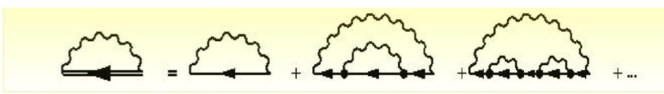
Figure 3: The coupling of the quasiparticle to many-phonon states, corresponding to the rainbow diagrams shown in the figure, is included in our approach through the iteration of the self-consistent diagonalization of the Nambu-Gor’kov matrix.

II.1.1 Energy dependent, BCS-like formulation

The diagonalization of the eigenvalue problem (1) is equivalent to the $2\times 2$ energy-dependent eigenvalue problem derived from an approach based on Green’s function formalism (cf. e.g. Ter:02 ):

$$\left(\matrix{E_{a}+\Sigma^{11pho}_{a(n)}&\Sigma^{12pho}_{a(n)}\cr\Sigma^{12pho}_{a(n)}&-E_{a}+\Sigma^{22pho}_{a(n)}}\right)\left(\matrix{x_{a(n)}\cr y_{a(n)}}\right)=\tilde{E}_{a(n)}\left(\matrix{x_{a(n)}\cr y_{a(n)}}\right)$$ (31)

where one has introduced the energy-dependent, normal self-energies $\Sigma^{11pho}_{a(n)}$ and $\Sigma^{22pho}_{a(n)}$ given by

$$\Sigma^{11pho}_{a(n)}=\sum_{b,m,\lambda,\nu}\frac{V^{2}(ab(m)\lambda\nu)}{\tilde{E}_{a(n)}-\tilde{E}_{b(m)}-\hbar\omega_{\lambda\nu}}+\sum_{b,m,\lambda,\nu}\frac{W^{2}(ab(m)\lambda\nu)}{\tilde{E}_{a(n)}+\tilde{E}_{b(m)}+\hbar\omega_{\lambda\nu}}$$ (32)

$$\Sigma^{22pho}_{a(n)}=\sum_{b,m,\lambda,\nu}\frac{W^{2}(ab(m)\lambda\nu)}{\tilde{E}_{a(n)}-\tilde{E}_{b(m)}-\hbar\omega_{\lambda\nu}}+\sum_{b,m,\lambda,\nu}\frac{V^{2}(ab(m)\lambda\nu)}{\tilde{E}_{a(n)}+\tilde{E}_{b(m)}+\hbar\omega_{\lambda\nu}}$$ (33)

and the abnormal self-energy

$$\Sigma^{12pho}_{a(n)}=-\sum_{b,m,\lambda,\nu}V(ab(m)\lambda\nu)W(ab(m)\lambda\nu)$$ (34)

$$\left[\frac{1}{\tilde{E}_{a(n)}-\tilde{E}_{b(m)}-\hbar\omega_{\lambda\nu}}-\frac{1}{\tilde{E}_{a(n)}+\tilde{E}_{b(m)}+\hbar\omega_{\lambda\nu}}\right].$$ (35)

We note that $\Sigma^{11}$ evaluated at a given energy $E$ is equal to $-\Sigma^{22}$ evaluated at $-E$, that is, $\Sigma^{11pho}_{a(n)}=-\Sigma^{22pho}_{a(-n)}$. The normalization of the quasiparticle strength of the $n$-fragment (cf. Eq. (2)) is given by Bloch

$$x_{a(n)}^{2}+y_{a(n)}^{2}-\frac{\partial\Sigma^{11pho}_{a(n)}}{\partial\tilde{E}_{a(n)}}x^{2}_{a(n)}-\frac{\partial\Sigma^{22pho}_{a(n)}}{\partial\tilde{E}_{a(n)}}y^{2}_{a(n)}-2\frac{\partial\Sigma^{12pho}_{a(n)}}{\partial\tilde{E}_{a(n)}}x_{a(n)}y_{a(n)}=1.$$ (36)

In this form one can easily make contact with the formalism based on the Green’s function for superfluid systems,

$$\hat{G}_{a}(\tilde{E}_{a}+i\delta)=[(\tilde{E}_{a}+i\delta){\bf 1}-E_{a}\tau_{3}-\hat{\Sigma}^{pho}_{a}(\tilde{E}_{a}+i\delta)]^{-1},$$ (37)

where $\tau_{3}$ denotes a Pauli matrix, and where

$$\hat{\Sigma}^{pho}_{a}(\tilde{E}_{a}+i\delta)=\left(\matrix{\Sigma^{11pho}_{a}(\tilde{E}_{a}+i\delta)&\Sigma^{12pho}_{a}(\tilde{E}_{a}+i\delta)\cr\Sigma^{12pho}_{a}(\tilde{E}_{a}+i\delta)&\Sigma^{22pho}_{a}(\tilde{E}_{a}+i\delta)}\right)$$ (38)

is our phonon-mediated self-energy matrix evaluated at the complex energy $\tilde{E}_{a}+i\delta$, which coincides with the matrix introduced by Nambu and extensively used in condensed matter to deal with strong coupling superconductivity Schr:64 . Eqs. (37),(38) must be solved self-consistently due to the fact that the quasiparticle strengths needed for the evaluation of $\hat{\Sigma}^{pho}_{a}(\tilde{E}_{a}+i\delta)$ through the $V$ and $W$ matrix elements are obtained from the imaginary part of $\hat{G}_{a}(E+i\delta)$ (cf. Sluys:93 , Eqs.(46-47)).

In order to get more insight concerning the respective contributions of the bare and of the phonon-induced interaction to the pairing gap, it is useful to rewrite the 2x2 eigenvalue problem (31) in terms of the amplitudes $\tilde{u},\tilde{v}$, instead of $x,y$, by inverting the relation (5), obtaining

$$\left(\matrix{(\epsilon_{a}-\epsilon_{F})+\tilde{\Sigma}^{11}_{a(n)}&\tilde{\Sigma}^{12}_{a(n)}\cr\tilde{\Sigma}^{12}_{a(n)}&-(\epsilon_{a}-\epsilon_{F})+\tilde{\Sigma}^{22}_{a(n)}}\right)\left(\matrix{\tilde{u}_{a(n)}\cr\tilde{v}_{a(n)}}\right)=\tilde{E}_{a(n)}\left(\matrix{\tilde{u}_{a(n)}\cr\tilde{v}_{a(n)}}\right),$$ (39)

where $\epsilon_{a}$ denotes the HF single-particle energy, while the new normal self-energies are given by

$$\tilde{\Sigma}^{11}_{a(n)}=u_{a}^{2}\Sigma^{11pho}_{a(n)}+v_{a}^{2}\Sigma^{22pho}_{a(n)}-2u_{a}v_{a}\Sigma^{12pho}_{a(n)}$$ (40)

$$\tilde{\Sigma}^{22}_{a(n)}=u_{a}^{2}\Sigma^{22pho}_{a(n)}+v_{a}^{2}\Sigma^{11pho}_{a(n)}+2u_{a}v_{a}\Sigma^{12pho}_{a(n)}.$$ (41)

One can separate the abnormal self-energy into two terms, writing

$$\tilde{\Sigma}^{12}_{a(n)}=\Delta^{BCS}_{a}+\tilde{\Sigma}^{12,pho}_{a(n)}.$$ (42)

The first term, $\Delta^{BCS}_{a}$, is the pairing gap associated with the bare interaction obtained in the HF+BCS calculation, while the second term is associated with the phonon-induced interaction and is given by

$$\tilde{\Sigma}^{12,pho}_{a(n)}=\Sigma^{12pho}_{a(n)}(u^{2}_{a}-v_{a}^{2})+u_{a}v_{a}(\Sigma^{11pho}_{a(n)}-\Sigma^{22pho}_{a(n)}).$$ (43)

Using Eqs. (30), (33) and (35) this expression can be simplified and the abnormal self-energy can be rewritten as

$$\tilde{\Sigma}^{12,pho}_{a(n)}=-\sum_{b,m}\frac{(2j_{b}+1)}{2}V_{ind}(a(n)b(m))\tilde{u}_{b(m)}\tilde{v}_{b(m)},$$ (44)

where we have introduced the induced pairing interaction:

$$V_{ind}(a(n)b(m))=\sum_{\lambda,\nu}\frac{2h^{2}(ab\lambda\nu)}{(2j_{b}+1)}\times$$ (45)

$$\left[\frac{1}{\tilde{E}_{a}(n)-\tilde{E}_{b}(m)-\hbar\omega_{\lambda\nu}}-\frac{1}{\tilde{E}_{a}(n)+\tilde{E}_{b}(m)+\hbar\omega_{\lambda\nu}}\right].$$ (46)

Furthermore, we can symmetrize the matrix (39) in order to get a $2\times 2$ eigenvalue equation which is formally identical to the BCS eigenvalue equation. This can be achieved multiplying Eq. (39) by the $Z_{a(n)}$ energy-dependent function,

$$Z_{a(n)}=\left(1-\frac{\tilde{\Sigma}^{odd}_{a(n)}}{\tilde{E}_{a(n)}}\right)^{-1},$$ (47)

where $\tilde{\Sigma}^{odd}$ is the odd part of $\tilde{\Sigma}^{11}_{a(n)}$

$$\tilde{\Sigma}^{odd}_{a(n)}=\frac{\tilde{\Sigma}^{11}_{a(n)}+\tilde{\Sigma}^{22}_{a(n)}}{2}=\frac{\Sigma^{11pho}_{a(n)}+\Sigma^{22pho}_{a(n)}}{2}.$$ (48)

We note that according to the definition above, $Z$ is the inverse of the correspondent quantity as defined in Ter:02 ,Schr:64 . We also note that the symbol $Z$ is often used instead of $N$ to define the quasiparticle strength. In fact the two quantities tend to take similar values close to the Fermi energy (cf. Fig. 7 below). This similarity can be explained, on the one hand, by noting that for the lowest pole, the finite difference in the expression of $Z$ can be approximated by a derivative:

$$Z_{a(n)}=\left(1-\frac{\Sigma^{11}_{a(n)}-\Sigma^{11}_{a(-n)}}{2\tilde{E}_{a(n)}}\right)^{-1}\approx\left(1-\frac{\partial\Sigma^{11}_{a(n)}}{\partial\tilde{E}_{a(n)}}\right)^{-1}.$$ (49)

On the other hand, in the normalization of the strength of quasiparticles close to the Fermi energy, $x>>y$ so that, using Eq. (36),

$$N_{a(n)}=x_{a(n)}^{2}+y_{a(n)}^{2}\approx x_{a(n)}^{2}\approx\left(1-\frac{\partial\Sigma^{11}_{a(n)}}{\partial\tilde{E}_{a(n)}}\right)^{-1}.$$ (50)

It is possible to rewrite Eq. (39) as

$$\left(\matrix{\tilde{\epsilon}_{a(n)}-e_{F}&\tilde{\Delta}_{a(n)}\cr\tilde{\Delta}_{a(n)}&-(\tilde{\epsilon}_{a(n)}-e_{F})}\right)\left(\matrix{\tilde{u}_{a(n)}\cr\tilde{v}_{a(n)}}\right)=\tilde{E}_{a(n)}\left(\matrix{\tilde{u}_{a(n)}\cr\tilde{v}_{a(n)}}\right)$$ (51)

where

$$\tilde{\epsilon}_{a(n)}-e_{F}=Z_{a(n)}\left[(\epsilon_{a}-e_{F})+\tilde{\Sigma}^{even}_{a(n)}\right],$$ (52)

and where $\tilde{\Sigma}^{even}_{a(n)}$ is the even part of $\tilde{\Sigma}^{11}_{a(n)}$:

$$\tilde{\Sigma}^{even}_{a(n)}=\frac{\tilde{\Sigma}^{11}_{a(n)}-\tilde{\Sigma}^{22}_{a(n)}}{2}=(u_{a}^{2}-v_{a}^{2})\frac{\Sigma^{11pho}_{a(n)}-\Sigma^{22pho}_{a(n)}}{2}-2u_{a}v_{a}\Sigma^{12pho}_{a(n)}.$$ (53)

The term $\tilde{\epsilon}_{a(n)}$ in Eq. (51) represents the renormalized single-particle energy, and one can now identify the pairing gap with the term $\tilde{\Delta}_{a(n)}$ Schr:64 :

$$\tilde{\Delta}_{a(n)}=Z_{a(n)}\tilde{\Sigma}^{12}_{a(n)}=Z_{a(n)}\left(\Delta^{BCS}_{a}+\tilde{\Sigma}^{12,pho}_{a(n)}\right)\equiv\tilde{\Delta}_{a(n)}^{bare}+\tilde{\Delta}_{a(n)}^{pho}.$$ (54)

This quantity coincides with the expression 6 introduced above, which can be used when solving the energy independent problem (1), because it involves only quasiparticle energies and amplitudes. Note also that the quasiparticle energy relates to the new gap and single-particle energy as in the usual BCS equations:

$$\tilde{E}_{a(n)}=\sqrt{(\tilde{\epsilon}_{a(n)}-e_{F})^{2}+\tilde{\Delta}^{2}_{a(n)}}$$ (55)

It is now possible to write a generalized gap equation. Introducing the total quasiparticle strength for a given fragment,

$$\tilde{u}^{2}_{a_{n}}+\tilde{v}^{2}_{a_{n}}=N_{a(n)},$$ (56)

the product $\tilde{u}_{a(n)}\tilde{v}_{a(n)}$ may be obtained in the usual way from the 2x2 secular equation as

$$\tilde{u}_{a(n)}\tilde{v}_{a(n)}=N_{a(n)}\frac{\tilde{\Delta}_{a(n)}}{2\sqrt{(\tilde{\epsilon}_{a(n)}-e_{F})^{2}+\tilde{\Delta}^{2}_{a(n)}}}.$$ (57)

$$\tilde{u}_{a(n)}\tilde{v}_{a(n)}=N_{a(n)}\frac{Z_{a(n)}\tilde{\Sigma}^{12}_{a(n)}}{2\sqrt{Z^{2}_{a(n)}(\epsilon_{a}-e_{F}+\tilde{\Sigma}^{even}_{a(n)})^{2}+(Z_{a(n)}\tilde{\Sigma}^{12}_{a(n)})^{2}}}.$$ (58)

Substituting in Eq. (44) one obtains

$$\tilde{\Sigma}^{12}_{a(n)}=\Delta_{a}-\sum_{b(m)}V_{ind}(anbm)N_{b(m)}\frac{\tilde{\Sigma}^{12}_{b(m)}}{2\sqrt{(\epsilon_{b}-e_{F}+\tilde{\Sigma}^{even}_{b(m)})^{2}+(\tilde{\Sigma}^{12}_{b(m)})^{2}}}.$$ (59)

The second term in this equation is a generalization of the usual BCS gap equation, and clearly demonstrates how the action of the different fragments of the original quasiparticles is modulated by their quasiparticle strength $N_{b(m)}$. The equation, however, is of little practical use as it stands because it involves the energy dependent interaction $V_{ind}$ which contains a ”dangerous” denominator (cf. Eq. (46)). The formula will be further discussed in Section III.1.4, and we shall present a similar expression in Section II.2 (cf. Eqs. 70-71).

The approach presented so far (and in Sluys:93 ) neglects the $1qp$-exchange interaction between the complex $1qp\otimes 1ph$ states (see fig. 6.10 c-d in BM:75 ). In fact the associated matrix elements are set to 0 in the matrix (1). The ignored processes would account for some violation of the Pauli principle arising from the microscopic structure of the QRPA phonons, which may imply double occupation of the quasiparticle state in the complex $1qp\otimes 1ph$ state. These violations are anyway very small for the calculation reported in this paper (cf. Section VI.4).

Those processes account also for vertex renormalization terms in the self-energy, which are not taken into account in the rainbow series we have considered. While in condensed matter they are usually neglected based on the Migdal theorem, in nuclear physics they are usually considered to be of minor importance because their contribution to the self-energy implies a recoupling of angular momenta that when summed up over all possible intermediate states is expected to lead to a rather strong cancellation belyaev ; avdeenkov . As we have mentioned discussing approximation (B) above, we shall assume that they are implicitely included in our effective PVC, computed making use of phenomenological phonons and single-particle levels.

Although within NFT tadpole diagrams should be included nft3 , we will neglect the energy-independent contributions associated with them (cf. Fig. 4), which take into account the effect of zero-point fluctuations on the quasiparticle energy khodel . This kind of diagrams modifies the nuclear density (cf. Fig. 5) and plays a particular important role in the calculation of nuclear radii barranco_radii ; khodel_radii ; fayans , representing the leading correction beyond mean field for closed shell nuclei, and producing sizeable isotopic effects barranco_plb . However, they lead to relatively small changes in the mean-field potential. The shifts of the single-particle energies for $A=120$ can be estimated to be of the order of 150 keV madurga , and, being of static nature, we shall assume that they are effectively taken into account in the mean field. The tadpole diagrams can also influence the abnormal density an the calculation of the bare pairing gap saperstein:08 , but no calculations have been performed for superfluid nuclei. We have estimated that the effect of diagrams (a) and (b) in Fig. 5 changes the abnormal density $\kappa$ by about 5%. This value can be obtained from the expression

$$\delta{\kappa}(r)=\sum_{ab\lambda}(2\lambda+1)Y_{ab\lambda}^{2}\kappa_{a}(r)/(2j_{a}+1),$$ (60)

where $Y_{ab\lambda}$ denotes a backward amplitude calculated in QRPA. The diagrams (c) and (d), in the normal case, give a contribution to the renormalization of the radius which is about three times larger than the one produced by (a) and (b) barranco_radii . This can be considered as an upper limit since the strong $r^{2}$ dependence tend to enhance their relative importance.

Thus we estimate a total tadpole effect to the pairing field of less than 20/value, that is less than 200 keV, which is a number rather consistent with that estimated above for the normal single-particle energy.

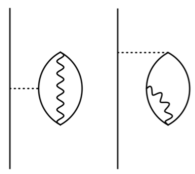
Figure 4: Lowest order diagrams representing the renormalization of the quasiparticle self-energy by zero-point fluctuations.

Figure 5: Lowest order diagrams representing the renormalization of the density operator (represented by the cross) by zero-point fluctuations in closed shell nuclei.

Finally, we note that the formalism presented in this Section is similar to the one adopted by Avdeenkov and Kamerdzhiev Avd:1 ; Avd:2 . However, a precise comparison of their results with ours is difficult, because they have followed a different approach, trying to extract ’bare’ single-particle levels and pairing gaps from the experimental levels, instead of renormalizing the levels obtained from an effective mean field.

II.2 The post scheme

In the previous Section we have outlined the prior scheme in the calculation of the pairing properties of superfluid nuclei. That is, we have started from a HF+BCS calculation which accounts for the bare pairing interaction and we have then added the effects of the PVC diagonalizing the matrix in Eq.(1). However one could also adopt a different scheme (which we will call the post-scheme) in which one starts from the HF solution and then one includes simultaneously both renormalization effects and the bare pairing interaction through the iterative procedure. This approach is particularly appropriate when the phonon induced pairing provides the leading contribution to pairing correlations, and is certainly needed when the bare interaction alone is not able to produce a superfluid solution. This is the case, for instance, in calculations of halo nuclei based on the PVC coupling noi:11li ; noi:11be . On the other hand, the prior-scheme is more natural, in the framework of general schemes based on the corrections to mean field properties.

In the following we shall apply the post scheme to the calculation of pairing properties in ¹²⁰Sn, which is a well bound, superfluid nucleus. In this case we expect that the two schemes should give similar results concerning physically relevant quantities, namely quasiparticle energies, spectroscopic factors and pairing gaps.

The calculation in the post scheme is performed by introducing the bare pairing field $\Sigma^{12bare}$ associated with the bare interaction in Eq.(1), by writing

$$\left(\matrix{E_{a}&V(ab\lambda\nu)&V(ac\lambda\nu)&W(ab\lambda\nu)&W(ac\lambda\nu)&\mp\Sigma^{12,bare}\cr V(ab\lambda\nu)&\hbar\omega_{\lambda\nu}+E_{b}&0&0&0&W(ab\lambda\nu)\cr V(ac\lambda\nu)&0&\hbar\omega_{\lambda\nu}+E_{c}&0&0&W(ac\lambda\nu)\cr W(ab\lambda\nu)&0&0&-\hbar\omega_{\lambda\nu}-E_{b}&0&-V(ab\lambda\nu)\cr W(ac\lambda\nu)&0&0&0&-\hbar\omega_{\lambda\nu}-E_{c}&-V(ac\lambda\nu)\cr\mp\Sigma^{12bare}&W(ab\lambda\nu)&W(ac\lambda\nu)&-V(ab\lambda\nu)&-V(ac\lambda\nu)&-E_{a}}\right)\left(\matrix{x_{a(n)}\cr C_{a(n),b,\lambda\nu}\cr C_{a(n),c,\lambda\nu}\cr-D_{a(n),b,\lambda\nu}\cr-D_{a(n),c,\lambda\nu}\cr-y_{a(n)}}\right)=$$

$$\tilde{E}_{a(n)}\left(\matrix{x_{a(n)}\cr C_{a(n),b,\lambda\nu}\cr C_{a(n),c,\lambda\nu}\cr-D_{a(n),b,\lambda\nu}\cr-D_{a(n),c,\lambda\nu}\cr-y_{a(n)}}\right)$$ (61)

where now the unperturbed ”quasiparticle” energy $E_{a}$ contains no contribution from pairing and is simply equal to the difference between the HF single-particle energy and the Fermi energy,

$$E_{a}=|{\epsilon_{a}-\epsilon_{F}}|,$$

where $\Sigma^{12bare}$ obeys the equation

$$\Sigma^{12bare}=-\sum_{b,n}V_{bare}(ab)\frac{(2j_{b}+1)}{2}\tilde{u}_{b(n)}\tilde{v}_{b(n)},$$ (62)

and the -(+) sign is to be used for particle-(hole-) states, that is $\epsilon_{a}>e_{F}$ ($\epsilon_{a}<e_{F}$).

The amplitudes $\tilde{u}_{a(n)},\tilde{v}_{a(n)}$ are given by Eq. (5), taking into account the fact that the initial $u_{a}$ and $v_{a}$ factors to be inserted in the iterative solution of Eq.(1) are now equal to 1 or 0, depending on whether the level is above or below the Fermi energy:

$$\tilde{u}_{a(n)}=x_{a(n)}\quad\tilde{v}_{a(n)}=y_{a(n)}$$ (63)

and

$$\tilde{u}_{a(n)}=-y_{a(n)}\quad\tilde{v}_{a(n)}=x_{a(n)}$$ (64)

respectively in the case of a particle- and a hole-state.

Note that, putting the $V-W$ matrix elements to zero, Eq. (62) reduces to the standard BCS equation for the pairing gap. The solution must be obtained through a self-consistent iterative procedure which in the general case involves simultaneously the bare interaction and the PVC vertices $V$ and $W$. In general this is not equivalent to the two-step diagonalization performed in the prior scheme, in which one considers first only $\Sigma^{12bare}$ (which is exactly equivalent to solve the bare BCS problem), and then takes into account the matrix elements $V$’s and $W$’s. Nevertheless we expect that the two schemes lead to similar results, as long as the first diagonalization leads to a finite value of the order parameter, the pairing gap.

As in the prior scheme one can use the $2\times 2$ energy dependent BCS-like matrix to solve the problem. The only difference with respect to Eq. (51) is that now the renormalized pairing gap must include a term $\Sigma^{12bare}$ representing the contribution of the bare pairing interaction:

$$\tilde{\Delta}_{a(n)}=Z_{a(n)}\left(\Sigma^{12bare}_{a(n)}+\tilde{\Sigma}^{12,pho}_{a(n)}\right)=\tilde{\Delta}^{bare}_{a(n)}+\tilde{\Delta}^{pho}_{a(n)}.$$ (65)

This expression can be rewritten in the more appealing way

$$\tilde{\Delta}_{a(n)}=-Z_{a(n)}\sum_{b,m}\frac{(2j_{b}+1)}{2}V_{eff}(a(n)b(m))\tilde{u}_{b(m)}\tilde{v}_{b(m)}=$$ (66)

where one has introduced the effective interaction $V_{eff}$, which is the sum of the bare and phonon-induced interactions:

$$V_{eff}(a(n)b(m))=V_{bare}(ab)+V_{ind}(a(n)b(m))$$ (67)

Furthermore one can obtain a very closed form for the gap equation by eliminating the amplitudes $u$ and $v$ using Eq. (51):

$$\tilde{u}_{a(n)}\tilde{v}_{a(n)}=N_{a(n)}\frac{\tilde{\Delta}_{a(n)}}{2\tilde{E}_{a(n)}}=N_{a(n)}\frac{Z_{a(n)}\tilde{\Sigma}^{12}_{a(n)}}{2\sqrt{Z^{2}_{a(n)}(\epsilon_{a}-e_{F}+\tilde{\Sigma}^{even}_{a(n)})^{2}+(Z_{a(m)}\tilde{\Sigma}^{12}_{a(n)})^{2}}}.$$ (68)

leading to

$$\tilde{\Delta}_{a(n)}=Z_{a(n)}\tilde{\Sigma}^{12}_{a(n)}=$$ (69)

$$-Z_{a(n)}\sum_{b(m)}\frac{2(j_{b}+1)}{2}V_{eff}(a(n)b(m))N_{b(m)}\frac{\tilde{\Sigma}^{12}_{b(m)}}{2\sqrt{(\epsilon_{b}-e_{F}+\tilde{\Sigma}^{even}_{b(m)})^{2}+(\tilde{\Sigma}^{12}_{b(m)})^{2}}}.$$ (70)

We note that for levels near to the Fermi energy the $Z-$factor is very close to the quasiparticle strength $N$. A more compact expression, bearing a direct resemblance to the standard BCS gap equation, may be obtained by reintroducing the $Z-$function both in the numerator and in the denominator:

$$\Delta_{a(n)}=-Z_{a(n)}\sum_{b(m)}V_{eff}(a(n)b(m))N_{b(m)}\frac{\Delta_{b(m)}}{2\tilde{E}_{b(m)}}.$$ (71)

This equation is an exact consequence of the Nambu-Gor’kov energy-dependent problem and can be used as an useful starting point for approximate gap equations (see Section III.1.4 ). In particular, restricting the sum to the main peak $m=1$ and neglecting the difference between $N$ and $Z$, Eq. (71) formally reduces to an approximate gap equation previously presented in the case of uniform matter (lombardo (cf. Eq.(12)), baldo ).

III Results

In the following we present the solution of the Nambu-Gor’kov equations for ¹²⁰Sn in various approximations. In all cases, we shall limit our attention to the five neutron levels belonging to the shell around the Fermi energy (namely, the 1$g_{7/2}$, the 2$d_{5/2}$, the 3$s_{1/2}$, the 2$d_{3/2}$ and the 1$h_{11/2}$ orbitals). Most of the calculations will be performed in the prior scheme, making use of the Argonne nucleon-nucleon interaction as the bare pairing force in the ${}^{1}S_{0}$ channel, which gives by far the dominant contribution to $T=1,J=0$ pairing baroni_gap . In Appendix VI.2 we shall also show a few results obtained with the $V_{{\rm low}k}$ potential.

In general we shall iterate the renormalization process. This requires looking for a self-consistent solution, either by successive diagonalizations of the matrix (1) or (61), or looking for the solutions of the equivalent energy-dependent $2\times 2$ problem (31). Nearly all of the results presented in this work have been obtained from the the diagonalization procedure. However, we have verified in several instances the numerical agreement between the two approaches. In order to control the iteration process, one must introduce a cutoff procedure, or perform some averaging, in order to avoid the exponential increase of the number of solutions, retaining at the same time the essential information vanneck:91 ,vanneck:93 . We shall make use of two simple numerical procedures. A cutoff procedure can be adopted when one solves the energy-dependent problem. In this case one can limit the number of solutions kept at each iteration, by selecting only those fragments carrying a quasiparticle strength larger than a given cutoff $N_{cut}$. An extreme case is represented by the so-called one-quasiparticle approximation, in which one keeps only the most important pole for each orbital $a$. We shall instead make use of the averaging procedure when we solve the energy-independent problem diagonalizing the matrices (1) or (61). In this case we define a number $N_{zones}$ of energy zones. The zones are generally not of the same size, but are chosen so as to reflect the main features of the quasiparticle strength function. After each iteration we collect all the strength obtained within a given energy zone into a single fragment, placed at the calculated average energy position. In this way, the number of solutions associated with a given orbital $a$ is kept fixed to $N_{dim}=2\times\left[N_{phon}\times N_{sps}\times N_{zones}+2\right]$, where $N_{phon}$ is the number of RPA solutions retained in the diagonalization and $N_{sps}$ is the number of single-particle levels considered.

We shall compute the PVC coupling by first performing a QRPA calculation with the separable force (20) for the multipolarities and parities $\lambda^{\pi}=2^{+},3^{-},4^{+}$ and $5^{-}$. In each case, the coupling constant as determined so as to reproduce the experimental value of the ratio $B(E\lambda)/\hbar\omega_{\lambda,1}$ (cf. the discussion about the approximation (B) in Section II above). Experimental data are taken from expdata_phon . The quasiparticle states used in the QRPA calculation are obtained from a BCS calculation with a monopole pairing interaction $-G_{0}P^{\dagger}P$ based on the levels of a Woods-Saxon potential parametrized as in ref. BM:69 , Eq. (2-182). The pairing coupling constant $G_{0}$ is adjusted so as to reproduce the value $\Delta_{exp}\approx 1.4$ MeV derived from the experimental odd-even mass difference. The PVC matrix elements are then obtained from Eq. (27).

Concerning the QRPA spectrum, we adopt an averaging procedure similar to that adopted for the quasiparticle strength. We include explicitly the strong collective low-lying vibrational states and we collect the remaining strength in a small number of peaks, reflecting the gross structure of the response for each multipolarity Ter:02 . We have verified that the results are not sensitive to the details of the high-lying phonons. The properties of the low-lying phonons employed in the calculations are listed in Table 1, where they are compared with the available experimental data. We remark that the values of $\chi_{\lambda}$ (cf. Eq. (20)) are close to 0.9, reflecting the rather good accuracy of the collective model.

	Exp.			Theory
$\lambda^{\pi}$	$\hbar\omega_{\lambda 1}$	$\beta_{\lambda 1}$	$\beta_{\lambda 1}^{2}/\hbar\omega_{\lambda 1}$	$\hbar\omega_{\lambda 1}$	$\beta^{eff}_{\lambda 1}$	$(\beta^{eff}_{\lambda 1})^{2}/\hbar\omega_{\lambda 1}$	$\chi_{\lambda}$
$2^{+}$	$1.17$	$0.13$	$0.014$	$1.20$	$0.13$	0.013	0.86
$3^{-}$	$2.40$	$0.16$	$0.011$	$2.71$	$0.16$	0.010	0.95
$4^{+}$	$3.10$	$0.11$	$0.004$	$2.33$	$0.10$	0.004	0.91
$5^{-}$	$2.27$	$0.08$	$0.003$	$2.48$	$0.09$	0.003	0.91

Table 1: In the first columns we list the experimental energies $\hbar\omega_{\lambda 1}$ in (MeV), deformation parameters $\beta_{\lambda 1}$ and polarizabilities $\beta^{2}_{\lambda 1}/\hbar\omega_{\lambda 1}$ of the low-lying states associated with the $2^{+}$, $3^{-}$, $4^{+}$ and $5^{-}$ multipolarities. They are compared with the corresponding quantities calculated in QRPA, making use of the effective deformation parameter $\beta^{eff}_{\lambda\nu}=\chi_{\lambda}\beta_{\lambda\nu}$. In the last column we give the values of $\chi_{\lambda}$. In the case of $4^{+}$, the experimental low-lying strength is fragmented in four peaks lying between 2.2 and 3.8 MeV; the numbers in the table refer to an average weighted with the transition strength of each peak.

III.1 Calculations with bare pairing potentials

In this Section, we shall discuss solutions of the Nambu-Gor’kov equations making use of bare nucleon-nucleon potentials as pairing interactions. As we have remarked above, we shall adopt the prior scheme. The practical difficulty with the post scheme is that the basis needed to account for the realistic bare interactions must span a broad energy interval (about 1 GeV in the case of the Argonne $v_{14}$ interaction, and about 200 MeV in the case of $V_{{\rm low}k})$. This implies a large numerical effort in order to handle Eq.(61), in particular because the matrix associated with a given angular momentum must include states with different number of nodes. We shall further consider the relation between the prior and post schemes presented in Section II, making use of a simplified bare interaction.

III.1.1 Bare pairing gap

The first step in our calculation is represented by the solution of the HF+BCS equation with the bare force in the pairing channel; we shall not consider the influence of pairing on the mean field.

We notice that the calculation with the bare force is in fact an extended BCS calculation, because for a hard-core interaction it is essential to consider the coupling between pairs of levels with different number of nodes, in order to take properly into account the coupling between bound and continuum levels noi_plb ; pizzo . We take into account states up to 1 GeV. As a consequence, for a given set of quantum numbers $a=\{lj\}$ one obtains a set of quasiparticles $\{E_{k}\}$; to each quasiparticle is associated an array of quasiparticle amplitudes $u_{nk}$ and $v_{nk}$, which are the components of the quasiparticle states over the HF basis states $\phi_{nlj}$. Going to the canonical basis, where the density matrix takes a diagonal form ring_schuck , we look for the state having the largest value of the abnormal density, $u_{max}v_{max}$. As a rule, for a stable nucleus like ¹²⁰Sn, this canonical state is dominated by the quasiparticle state having the lowest value of the quasiparticle energy, $E_{min}$. We then approximate the extended BCS calculation associating the value of $v_{max}$ and $E_{min}$, treating them as proper BCS quantities; in particular we derive an associated pairing gap as $\Delta^{BCS}=2u_{max}v_{max}E_{min}$, which is very close to the diagonal value of the gap in the original basis. The value of $v_{max},E_{min}$ and $\Delta^{BCS}$ are then employed as input values for the solution of the Nambu Gor’kov equations in the prior scheme described in Section II.1 (cf. Eqs. (1) and (5), where they are denoted $u_{a},v_{a}$ and $E_{a}$). This approximation leads to a substantial simplification of our numerical scheme. For nuclei close to the line of stability, where the canonical states have significant weight on continuum state and the PVC easily connects bound and continuum states, this approximation would not be justified and one should rather consider different numerical schemes, for example based on the continuum Green’s function.

The mean field will be taken from a HF calculation with the SLy4 interaction chabanat . This interaction gives a good reproduction of the bulk properties of nuclei; moreover the resulting level density close to the Fermi energy (associated with an effective mass $m_{k}\approx 0.7m$), once increased by renormalization effects, is in reasonable agreement with the experimental one (the associated effective mass increasing to $m^{*}=m_{k}m_{\omega}\approx m$). The energies of the five single-particle levels lying closest to the Fermi energies are shown in Appendix VI.1 (cf. Fig. 19). The detailed features of our calculations are of course influenced by the specific properties of the mean field, and in particular by its effective mass. In order to have some insight about the dependence on the adopted mean field, in the Appendix VI.1 we provide results obtained making use of two different Skyrme interactions, having effective masses smaller and larger than the SLy4 interaction. One should distinguish two different effects that influence the pairing gap calculated with the bare pairing interaction: on the one hand, the pairing gap is sensitive to the detailed position of the levels close to the Fermi energy, that could be influenced by static contributions not considered here, as those produced from tensor correlations duguet_tensor ; colo_tensor and from tadpole diagrams saperstein:08 (for the latter, cf. the comments at the end of Section II.1); on the other hand, the pairing gap is also sensitive to the momentum dependence of $m_{k}$ for large momenta.

In a previous work epj:04 we presented a solution of the HFB equations using the Argonne $v_{14}$ equation in the pairing channel, which led to a pairing gap of the order of 700 keV. There we used a modified SLy4 mean field, reducing the spin-orbit coupling strength by about 15% (furthermore we included in the Hamiltonian the terms proportional to the square of the spin density, which will not be included in the following, and used a slightly larger PVC strength). This was done, in order to improve the agreement of the results obtained after renormalization with the experimental spectrum and pairing gap. Here we prefer to take the HF field obtained with the original SLy4 interaction. This is associated with a larger level density around the Fermi energy. As a consequence, the obtained pairing gap, shown in Fig. 6 (full dots), is larger, being equal to about 1.1 MeV. Similar calculations have been performed with the $V_{{\rm low}k}$ potential using the same mean field hebeler . In that case, the result depends on the cutoff $\Lambda$ adopted to obtain $V_{{\rm low}k}$: for values of $\Lambda$ smaller than about 4 fm^-1, the gap is close to 1.4 MeV, (cf. Fig. 25), while for increasing values of $\Lambda$ the $V_{{\rm low}k}$ potential reduces to the Argonne potential and one obtains the result shown in Fig. 6. We notice that our numerical results with the Argonne potential are in very good agreement with those reported in ref. hebeler for very large values of $\Lambda$. The reason for the difference between the results obtained with the Argonne and $V_{{\rm low}k}$ interaction has been discussed in detail hebeler ; saperstein : using the Argonne potential implies using the Skyrme effective mass $m_{k}$ (equal to about 0.7$m$ inside the nucleus) up to very high momenta, while the renormalization process leading to $V_{{\rm low}k}$ implies that $m_{k}$ goes to the free mass for momenta larger than the cutoff $\Lambda$. The lower value of $m_{k}$ at high momenta leads to a smaller level density and to a reduction of about 300 keV in the value of the gap with the Argonne interaction with respect to the values obtained with $V_{{\rm low}k}$ for cutoffs $\Lambda$ up to about $4$fm^-1. An analogous difference shows up in calculation of the gap in uniform matter. While the lack of momentum dependence of the effective mass associated with Skyrme interactions is certainly unrealistic, the proper momentum dependence is still to be established; and the density dependence of $m_{k}$ associated with the SLy4 interaction in nuclear matter is not far from that resulting at the Fermi energy from calculations based on Brückner theory saperstein . Furthermore, a precise determination of the value of the bare gap within the $V_{{\rm low}k}$ scheme requires the consideration of the effects of the three-body force, which is expected to provide a repulsive contribution lombardo_three . A calculation of three-body effects within the $V_{{\rm low}k}$ renormalization scheme duguet_three ; duguet_threea leads in fact to a reduction of the gap, down to values close to those obtained with the Argonne interaction in Fig. 6. An average value of the bare gap close to 1 MeV was also derived in the analysis of refs. Avd:1 ; Avd:2 .

We have brought circumstantial evidence which testifies to the fact that a pairing gap $\Delta^{BCS}\approx$ 1.1 MeV for the levels around the Fermi energy obtained using the $v_{14}$ potential as bare pairing interaction and the effective mass associated with SLy4 represents a reasonable starting point, being well aware that the determination of the mean field and of the associated effective mass is one of the most important issues which remains to be fully clarified, for a quantitative and microscopic calculation of the gap in finite nuclei. In Section VI.1 we investigate the dependence of the results on the adopted mean field, whille in Section VI.2 we provide some results obtained adopting $V_{\rm{low}k}$ as bare pairing interaction.

III.1.2 Solution of the Nambu-Gor’kov equations

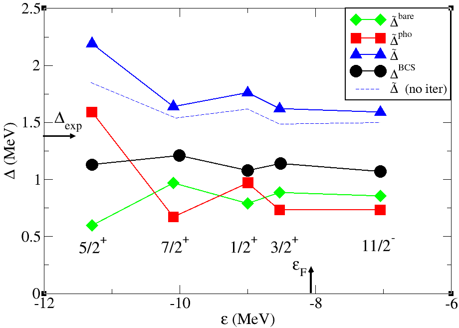
Figure 6: The state-dependent neutron paring gap $\Delta^{BCS}$ calculated in BCS with the bare $v_{14}$ interaction is shown as a function of the SLy4 HF single-particle energy of the five valence orbitals (cf. Fig. 19), and is compared to the renormalized gap $\tilde{\Delta}$ (cf. Eq. (54) ) obtained solving the Nambu-Gor’kov equations by iteration; also shown (dashed line) is the gap obtained at the first iteration. We also show the decomposition of $\tilde{\Delta}$ into the bare and phonon contributions $\tilde{\Delta}^{bare}$ and $\tilde{\Delta}^{pho}$. The value of the Fermi energy $\epsilon_{F}$ and of the gap obtained from the experimental odd-even mass difference $\Delta_{exp}$ are also indicated.

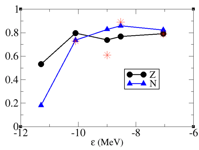
Figure 7: Comparison of the $N-$ and $Z-$ factors associated with the lowest quasiparticle peaks in the Nambu-Gor’kov calculation shown in Fig. 6. Also shown by stars are the values of the experimental quasiparticle strength exp_transf2 , except for the $d_{5/2}$ orbital which shows a pronounced fragmentation (cf. text).

The state-dependent pairing gap obtained from the solution of the Nambu-Gor’kov equations is compared to the bare gap in Fig. 6. Renormalization effects lead to a total gap $\tilde{\Delta}$ about 600 keV larger than $\Delta^{BCS}$. Most of the effect is obtained already with the first diagonalization of the Nambu-Gor’kov matrix. The self-consistent iteration process leads to a further increase of the gap by about 10%. We recall that one can distinguish two contributions to the renormalized gap $\tilde{\Delta}=Z[\Delta^{BCS}+\tilde{\Sigma}^{12,pho}]=\tilde{\Delta}^{bare}+\tilde{\Delta}^{pho}$, associated with the bare and with the phonon-induced interaction (cf. Eq. (54)). They are also shown in Fig. 6 and turn out to be of similar magnitude. This confirms that the phonon-induced pairing interaction is as important as the bare interaction in determining pairing properties of heavy nuclei. Notice that a proper comparison between the role of these two sources of pairing can only be made analyzing their contribution to the final physical result, and not just by comparing the BCS and complete pairing gaps. In fact, processes beyond mean field act in a complex way, not only giving rise to the induced pairing interaction, but also reducing the effect of the bare interaction through the $Z-$factors. The values of $Z$ for the five orbitals are shown in Fig. 7 where it can be seen that they are close to 0.7, bringing the bare contribution from the BCS result (about 1.1 MeV) down to about 0.8 MeV, which is about one half of the total renormalized gap. The other half is provided by the pairing induced interaction. The values of $Z$ are similar to the values of the quasiparticle strength $N=U^{2}+V^{2}$, except for the orbital $d_{5/2}$. The values of $N$ are in rather good agreement with the quasiparticle strength measured in one-nucleon transfer reactions, shown by stars in Fig. 7 (cf. also below Figs. 9 and 10 with the related discussion), although one has to consider that the experimental values are affected by a large error, estimated to be about 30%.

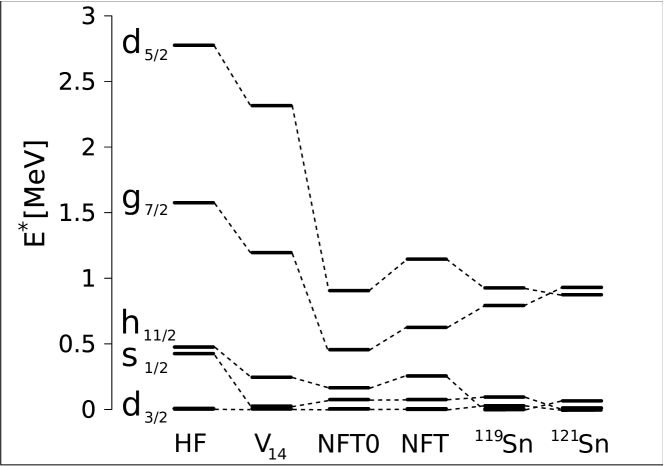
Figure 8: The theoretical quasiparticle spectra obtained at the various steps of the calculation are compared to the experimental data. See the text for more explanation.

The renormalized pairing gap exceeds the experimental value obtained from the odd-even mass difference by about 300 keV, the value of $\Delta_{exp}$ lying in between $\Delta^{BCS}$ and $\tilde{\Delta}$. We remark that the estimate of $\Delta_{exp}$ varies by about $\pm$ 100 keV depending on which odd-even mass formula is used bender ; duguet_oddeven ( the five-point formula $\Delta^{(5)}$ yielding a value of 1.39 MeV), and that a more consistent comparison would imply a theoretical calculation of the binding energies. Such a precise comparison of the gaps is probably not very significant at the present stage of the theory, given the uncertainties which affect both the BCS calculation - like the dependence on the adopted HF mean field and the effect of three-body forces mentioned above - and the renormalization process - in particular the exchange of spin modes, not included in this calculation (see the discussion in Section III.1.3 and Section IV.1). However, the fact that the value of the renormalized pairing gap is found to be relatively close to experiment is satisfactory. The necessity of going beyond mean field turns out anyway to be clearer considering other physical quantities, in particular the energy spectrum of neighbouring odd nuclei with the associated strength functions and spectroscopic factors. This can be seen in Fig. 8 where we compare the features of the quasiparticle spectrum obtained at the different steps of the calculation. In the first column (HF), we report the absolute value of the difference $|\epsilon_{a}-\epsilon_{F}|$ obtained in the HF calculation with the SLy4 force, referred to the value of this difference for the level $d_{3/2}$, which lies closest to the Fermi energy $\epsilon_{F}$ = -8.05 MeV (cf. Fig. 19). In the second column (BCS), we give the values of the quasiparticle energies obtained in the HF+BCS calculation with the Argonne force, referred to the lowest quasiparticle. In the third column (NFT0) we show the spectrum obtained taking into account processes beyond mean field calculated with the Nambu-Gor’kov equations without iterating, while in the fourth (NFT) we show the self-consistent solution: in these cases we show the energy of the lowest fragment for each quantum number (this is also the one collecting the largest quasiparticle strength, except for the $d_{5/2}$ orbital, which is very fragmented and whose case is discussed below): Finally in the fifth and sixth columns we give the position of the lowest peaks measured in ¹¹⁹Sn and ¹²¹Sn. The main discrepancy of the renormalized spectrum concerns the $7/2^{+}$ state, whose position is brought too low by the PVC by about 300 keV ( this is probably related to the initial position of the $g_{7/2}$ orbital in the HF spectrum, which lies too close to the Fermi energy, cf. Fig. 19). The experimental energies of the lowest three states are very close to each other, being separated by less than 100 keV, and are well separated by the other two levels. This gross structure is already present in the HF result, which, however, greatly underestimates the density of levels. This remains the case including pairing correlations at the BCS level (see second column), which lead to a limited improvement. The PVC leads to a denser spectrum, considerably improving the agreement with experiment, although one should not expect a detailed agreement in the order of three lowest levels. The main effect is already obtained with a single diagonalization (NFT0), but the self-consistent treatment leads to an appreciable rearrangement of the spectrum, somewhat reducing the initial compression of the levels, slightly improving the agreement with experiment. The increase of level density can be expressed as an increase of the neutron effective mass from $m^{*}\approx 0.7m$ to $m^{*}\approx m$. One could argue that a mean field BCS calculation in a potential with $m^{*}=1$ could lead to agreement with experiment in a simpler and more direct way. However, such a calculation (still performed with the bare interaction) would greatly overestimate the gap esb . Thus, the simultaneous consideration of gap and low-energy spectra clearly favours a description that includes renormalization effects on both quantities.

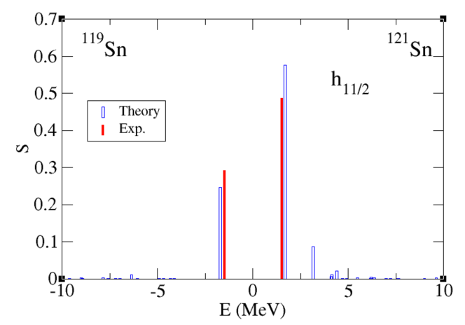
Figure 9: The theoretical strength function calculated for the $h_{11/2}$ orbital is compared to the spectroscopic factors associated with experimental levels detected in one-neutron transfer reactions.

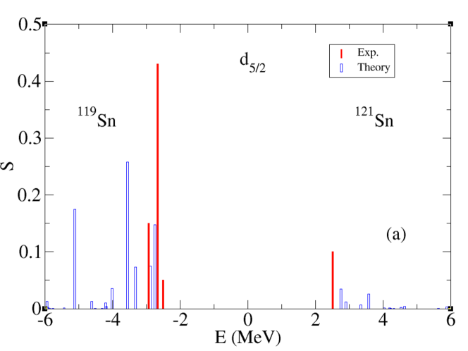
Figure 10: The theoretical strength function calculated for the $d_{5/2}$ orbital is compared to the spectroscopic factors associated with experimental levels detected in one-neutron transfer reactions.

The most specific fingerprint of the renormalization processes is represented by the fragmentation of the quasiparticle strength, that in our approach is due to the coupling with $1qp\otimes 1ph$ states. Experimentally, the effects of such a fragmentation leads to a breaking of the observed quasiparticle strength into several peaks, and consequently to a reduction of the strength observed in the main peaks, as compared to the full strength expected in mean field calculations. In the present case, strength functions measured in one-neutron transfer experiments involving ¹¹⁹Sn or ¹²¹Sn exp_transf1 ; exp_transf2 ; exp_transf3 show a strong, isolated peak for the quantum numbers $J^{\pi}=1/2^{+},3/2^{+},7/2^{+},11/2^{-}$. The case of $11/2^{-}$ is shown in Fig. 9, where we compare the theoretical values of $\tilde{v}^{2}$ ($\tilde{u}^{2})$ with the observed peak in ¹¹⁹Sn (¹²¹Sn). Here, and in similar figures, in order to compare the experimental to the theoretical strength functions, we have added the energy of the lowest calculated quasiparticle to the experimental excitation energy in the odd nuclei ¹¹⁹Sn and ¹²¹Sn. The summed strength of the two main peaks is equal to 0.79 in experiment and to 0.8 in theory. The remaining theoretical strength is calculated to lie at higher energy in ¹²¹Sn. A good agreement between theory and experiment is found also in the case of the other three quantum numbers, as was shown in Fig. 7.

It is interesting to notice that the main contribution to the renormalization effects originates from the coupling to the lowest vibrational state of each multipolarity : this demonstrates the key role played by the interweaving of collective and single-particle modes which is at the basis of the NFT treatment of the elementary modes of nuclear excitation. This is clearly seen in Fig. 11, where we compare the full calculations with results obtained including only couplings to the lowest vibrational states. It is seen that the coupling to the $2^{+}$ low-lying mode is the dominant one, providing half of the increase of the gap due to the renormalization effects. The other low-lying modes provide about one-third of the remaining increase of the gap, while higher energy modes (mainly giant resonances) complete the picture. The strength of the various PVC couplings is reported in Table 2, where for each pair of orbitals $(a,b)$ we list the value of the squares of the PVC matrix elements summed over the phonons of a given multipolarity, $\sum_{\nu}h^{2}(ab\lambda\nu)/(2j_{b}+1)$. We observe that although the deformation parameter associated with the lowest $3^{-}$ state is the largest one (cf. Table 1) its influence is hindered with respect to the $2^{+}$ by its higher energy and by the fact that it acts efficiently only between the $d_{5/2}$ and the $h_{11/2}$ orbitals, which are the only ones having opposite parity and the same spin alignment. We also note that the dominance of the coupling to low-lying vibrational states found in the present calculation makes our approach distinctly different from other approaches based on microscopic calculations of the PVC with zero-range forces, which need an energy cutoff to avoid an ultraviolet divergence in the self-energy colo:10 .

The strength of the remaining orbital, $5/2^{+}$, is much more fragmented both in theory and experiment, as is shown in Fig. 10. The experiment shows a number of low-energy peaks, which exhaust about 63% of the strength. The theoretical distribution is more fragmented than observed in the data; moreover most of the strength lies about 1 MeV above the experimental findings. In the calculation, the energy of the $d_{5/2}$ quasiparticle is lowered by its strong coupling with $s_{1/2}$ state (through the $2^{+}$ vibrations) and with the $h_{11/2}$ state (through the $3^{-}$ vibrations), as can be seen in Table 2. These couplings bring the energy of the $d_{5/2}$ state close to the energies of the $s_{1/2}\otimes 2^{+}_{1}$ and $d_{3/2}\otimes 2^{+}_{1}$ configurations. The matrix elements of the induced interaction $V_{ind}$ (cf. Eq. (46)) are listed in Table 3. They are calculated using the values of the renormalized quasiparticle energies $\tilde{E}_{a}(1)$ of the lowest fragment for each orbital. Their values can be compared to the typical value of the matrix elements of the bare interaction, which is about $G_{0}=-0.22$ MeV (cf. below Section III.2). They are rather well correlated with the PVC matrix elements reported in Table 2, with the remarkable exception of $d_{5/2}$: in the latter case, the induced interaction with the orbitals $s_{1/2}$ and $d_{3/2}$ takes large values, associated with the almost degeneracy of the energy of the $d_{5/2}$ quasiparticle with the configurations $s_{1/2}\otimes 2^{+}_{1}$ and $d_{3/2}\otimes 2^{+}_{1}$, which leads to the fragmentation of the $d_{5/2}$ strength.

These results may indicate that the unperturbed quasiparticle energy of the $d_{5/2}$ orbital lies too high. In fact, moving the energy of the single-particle energy by 600 keV towards the Fermi energy, and leaving everything else unchanged, and then solving the BCS and Nambu-Gor’kov equations, one obtains a better agreement with experiment, as will be shown below in Section IV.1 (cf. Fig. 18(d)). This shows that a detailed study of the fragmentation process can give important indications about how to improve the mean field (cf. also Section VI.1).

	$d_{5/2}$	$g_{7/2}$	$s_{1/2}$	$d_{3/2}$	$h_{11/2}$
$d_{5/2}$	$0.190$	$0.016$	$0.467$	$0.071$	$0.340$
	$0.088$	$0.041$	$0.$	$0.266$	$0.138$
$g_{7/2}$	$0.016$	$0.130$	$0.$	$0.236$	$0.020$
	$0.041$	$0.071$	$0.168$	$0.081$	$0.043$
$s_{1/2}$	$0.467$	$0.$	$0.$	$0.461$	$0.$
	$0.$	$0.168$	$0.$	$0.$	$0.389$
$d_{3/2}$	$0.071$	$0.236$	$0.461$	$0.253$	$0.$
	$0.266$	$0.081$	$0.$	$0.$	$0.092$
$h_{11/2}$	$0.340$	$0.020$	$0$	$0.$	$0.169$
	$0.138$	$0.043$	$0.389$	$0.092$	$0.100$

Table 2: For each pair $(a,b)$ of the five valence orbitals, we list the value of the sum $\sum_{\nu}h^{2}(ab\lambda\nu)/(2j_{b}+1)$, in MeV². For pairs of orbitals of the same parity, the numbers in the upper (lower) row give the contribution associated with $\lambda=2^{+}$ ($\lambda=4^{+}$) phonons; for pairs of orbital of different parity, the numbers in the upper (lower) row give the contribution associated with $\lambda=3^{-}$ ($\lambda=5^{-}$) phonons.

	$d_{5/2}$	$g_{7/2}$	$s_{1/2}$	$d_{3/2}$	$h_{11/2}$
$d_{5/2}$	$-0.223$	$-0.031$	$-1.701$	$-1.230$	$-0.309$
	$-0.054$	$-0.030$	$0.$	$-0.245$	$-0.075$
$g_{7/2}$	$-0.015$	$-0.157$	$0.$	$-0.513$	$-0.016$
	$-0.023$	$-0.045$	$-0.117$	$-0.062$	$-0.021$
$s_{1/2}$	$-0.383$	$0.$	$0.$	$-0.686$	$0.$
	$0.$	$-0.100$	$0.$	$0.$	$-0.177$
$d_{3/2}$	$-0.055$	$-0.219$	$-0.503$	$-0.319$	$0.$
	$-0.139$	$-0.047$	$0.$	$0.$	$-0.041$
$h_{11/2}$	$-0.183$	$-0.012$	$0$	$0.$	$-0.212$
	$-0.051$	$-0.017$	$-0.167$	$-0.042$	$-0.067$

Table 3: Matrix elements of the induced interaction $V_{ind(a(1)b(1))}$ (cf. Eq. (46)) between the lowest fragments of the five valence orbitals, in MeV. For pairs of orbitals for the same parity, the numbers in the upper (lower) row give the contribution of the matrix elements involving $2^{+}$ ($4^{+}$) phonons; for pairs of orbital of different parity, the numbers in the upper (lower) row give the contribution of the matrix elements involving $3^{-}$ ($5^{-}$) phonons.

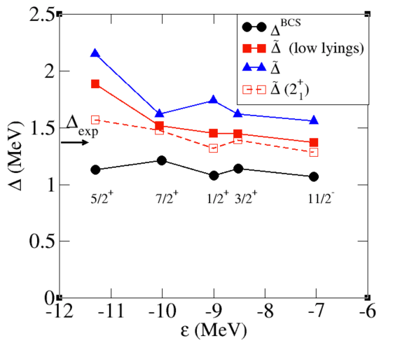
Figure 11: The pairing gaps $\Delta^{BCS}$ obtained in the BCS calculation (dots) and $\tilde{\Delta}$ including the renormalization effects (triangles) are compared to those obtained including only the renormalization due to the coupling to the lowest $2^{+},3^{-},4^{+}$ and $5^{-}$ QRPA modes (filled squares), or only the lowest $2^{+}$ mode (open squares).

III.1.3 Effects of spin modes

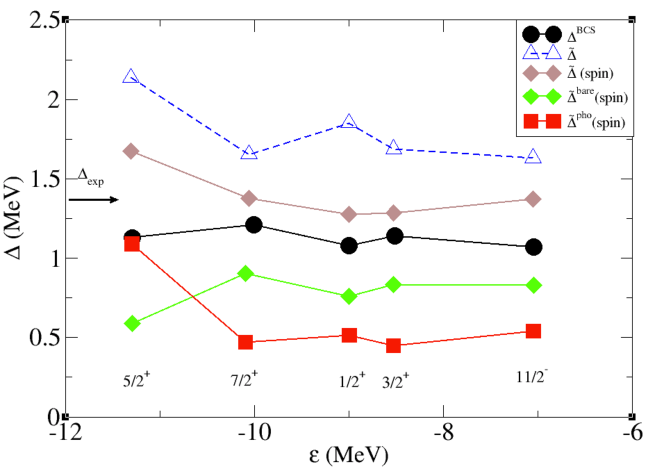
Figure 12: The BCS (dots) and renormalized pairing gaps associated with the lowest quasiparticle peaks obtained solving the Nambu-Gor’kov equations (triangles, cf. Fig. 6) are compared to the gaps obtained including the schematic spin-induced interaction discussed in the text (diamonds), and to their decomposition into $\tilde{\Delta}^{bare}$ and $\tilde{\Delta}^{pho}$.

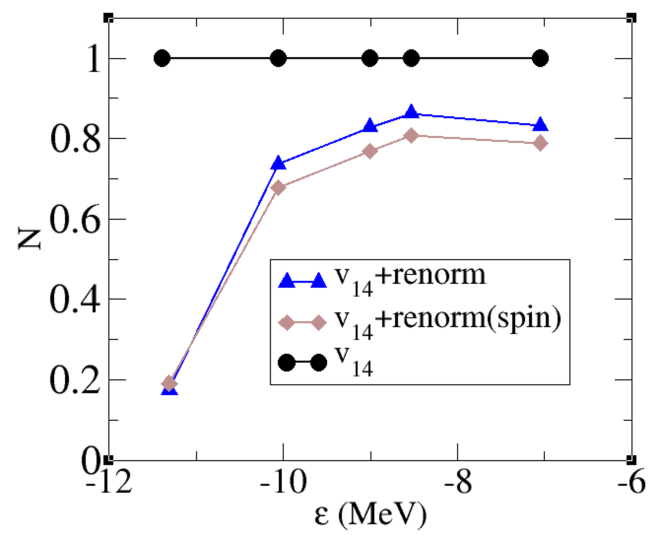
Figure 13: The strength $N$ associated with the main quasi particle peaks in the bare HF+BCS calculation (dots) and solving the Nambu-Gor’kov equations (triangles) is compared to the result obtained including the schematic spin-induced interaction discussed in the text (diamonds).

It is interesting to speculate about the effect of $S=1$ modes, that should be included in a more complete calculation. Their contribution represents the leading renormalization effect in calculations in uniform neutron matter, where it induces a repulsive contribution on the pairing interaction that wins over the attractive contribution associated with density modes - thanks to the larger multiplicity of spin modes - leading to a quenching of the pairing gap chen -viverit . On the other hand, one expects that the relative weight of spin modes should be considerably less important in finite nuclei, where there is no spin equivalent to low-lying surface collective vibrations.

The repulsive character of spin modes, as opposed to density modes, arises from their different transformation properties under time reversal. This is reflected in a sign change in the basic $V,W$ vertices (cf. Eq. (6-207) in BM:75 ), which become (cf. Eq. (30))

$$V(ab(m)\lambda\nu)= h_{S=1}(ab\lambda\nu)(u_{a}\tilde{u}_{b,m}+v_{a}\tilde{v}_{b,m})$$ (72)

$$W(ab(m)\lambda\nu)= h_{S=1}(ab\lambda\nu)(-u_{a}\tilde{v}_{b,m}+v_{a}\tilde{u}_{b,m}).$$ (73)

As a consequence. the product $VW$ which determines the abnormal self-energy $\Sigma^{12pho}$ (cf. Eq. (35)) also changes its sign, leading to a repulsive contribution. On the other hand the normal self-energies depend on the square of $V$ and $W$ so that their value is increased by the action of spin modes. There is furthermore a change in the expression of the basic vertex $h$, which is given by

$$h_{S=1}(abJ\nu)=-(-1)^{j_{a}-j_{b}}\beta_{J\nu}<a|f_{J}(r)|b><j_{b}||(Y_{\lambda}\sigma)_{J}||j_{a}>\left[\frac{1}{(2j_{a}+1)(2J+1)}\right]^{1/2},$$ (74)

where $f_{J}(r)$ is the form factor associated to the S=1 modes transition density.

The contribution of spin modes to pairing correlations in ¹²⁰Sn was estimated in ref. Gori:05 , based on a QRPA calculation performed with the SkM^∗ interaction. There it was found that, performing a calculation of the pairing gap including only the induced interaction, using the simplified expression discussed in Section III.1.4 (cf. Eq. (79)), the spin modes decreased the gap arising from the coupling with $S=0$ modes by about 25%. We have incorporated this effect in our present calculation by introducing a schematic $S=1$ response function, consisting of a single peak at an energy of about $1\hbar\omega_{osc}$, in keeping with the fact that there are no low-lying collective $S=1$ modes in finite nuclei. We have used an average value for the product $\beta_{J\nu}$ $<a|f_{J}(r)|b>$, treating it as an adjustable parameter in order to reproduce the 25% reduction in $\tilde{\Sigma}^{12pho}$ mentioned above, when no bare interaction is included. In this way we can estimate the effects of $S=1$ modes on the total gap and on the quasiparticle energies and strengths calculated in the present paper.

The values obtained for $\tilde{\Delta}$ and for the quasiparticle strength $N$ are shown respectively in Figs. 12 and 13. In keeping with their contribution to the normal self-energy, the action of spin modes tends to reduce, although slightly, the value of $Z$ and $N$, not modifying significantly the agreement with experiment. Spin modes also lead to a reduction of $\tilde{\Delta}^{pho}$ by about 25% (150 keV), which reflects directly the reduction introduced in $\tilde{\Sigma}^{12pho}$, while the value of $\tilde{\Delta}^{bare}$ is practically unaffected. Altogether, this brings the value of $\tilde{\Delta}$ closer to the experimental value of $\Delta_{exp}$= 1.4 MeV, without deteriorating the agreement with the experimental quasiparticle strength.

III.1.4 One-quasiparticle approximation and the gap equation

We have seen that the quasiparticle strength function for the states close to the Fermi energy displays a limited amount of fragmentation. If one is only interested in the properties of the main quasiparticle peaks, it may be interesting to solve the Nambu-Gor’kov problem by keeping only the main quasiparticle for each orbital in the iteration process. One then gets an excellent agreement with the complete calculation for the quasiparticle gap $\tilde{\Delta}_{a}^{q.p.}=Z_{a}\tilde{\Sigma}_{a}^{12,q.p.}$, as shown in Fig. 14: the result cannot be distinguished from the calculation for $\tilde{\Delta}$ shown in Fig. 6.

In order to have more insight on these results, we recall the gap equation Eq.(59):

$$\tilde{\Sigma}^{12}_{a(n)}=\Delta_{a}^{BCS}-\sum_{b(m)}V_{ind}(anbm)N_{b(m)}\frac{\tilde{\Sigma}^{12}_{b(m)}}{2\sqrt{(\epsilon_{b}-e_{F}+\tilde{\Sigma}^{even}_{b(m)})^{2}+(\tilde{\Sigma}^{12}_{b(m)})^{2}}}.$$ (75)

While the implementation of the quasiparticle approximation is straightforward, it is important to notice that in order to get good agreement one must include the factors $N$ and $Z$ associated with the quasiparticle peaks. Neglecting them, that is, attributing the full quasiparticle strength to the single peak retained in the calculation, leads to an increase of the gap by about 50%, in keeping with the typical values $Z\approx 0.7$, $N\approx 0.8$. Neglecting $N$ produces a smaller effect than neglecting $Z$, because $N$ affects only the induced part of the gap in Eq. (75). The error is especially pronounced for the case of $d_{5/2}$, where the one-quasiparticle approximation selects the lowest peak, which is associated with a small value of $N$ and $Z$ (cf. Fig. 7). From this result, one concludes that the gap receives only very small contributions from the fragments with $m>1$, which, on the other hand, account for more than 20% of the quasiparticle strength. This is mostly due to the energy dependence of $V_{ind}$, which is strongly peaked at the Fermi energy noi_schuck .

A gap equation equivalent to Eq. (75) has been obtained in the post scheme (cf. Eq. (71)):

$$\Delta_{a(n)}=-Z_{a(n)}\sum_{b(m)}V_{eff}(a(n)b(m))N_{b(m)}\frac{\Delta_{b(m)}}{2\tilde{E}_{b(m)}}.$$ (76)

This expression lends itself to approximations, which are useful in order to make a connection with previous works about renormalization effects on pairing. The most important feature of these approximations is the use of simplified expressions for the induced interaction $V_{ind}$ (cf. Eq. (46)),

$$V_{ind}(a(n)b(m))=\sum_{\lambda,\nu}\frac{2h^{2}(ab\lambda\nu)}{(2j_{b}+1)}\times$$ (77)

$$\left[\frac{1}{\tilde{E}_{a}(n)-\tilde{E}_{b}(m)-\hbar\omega_{\lambda\nu}}-\frac{1}{\tilde{E}_{a}(n)+\tilde{E}_{b}(m)+\hbar\omega_{\lambda\nu}}\right],$$ (78)

based on the Feynman diagram (1c) in Fig. 1 and neglecting fragmentation:

$$V_{ind}(ab)\approx\sum_{\lambda,\nu}\frac{2h^{2}(ab\lambda\nu)}{(2j_{b}+1)}\frac{2}{E_{0}-\tilde{E}_{a}-\tilde{E}_{b}-\hbar\omega_{\lambda\nu}},$$ (79)

in which $\tilde{E}_{a}=|\epsilon_{a}-\epsilon_{F}|$ and $E_{0}$ is the pairing energy per Cooper pair (equal to about - $2\Delta$) prl_noi . This expression was inserted in the BCS gap equation, without taking explicitly into account the renormalization effects on the single-particle density, namely, setting the $N$- and $Z-$ factors equal to one, and using a mean field potential characterized by an effective mass $m^{*}=m$. One then found gaps about 20% larger than those obtained solving the Nambu-Gor’kov equations Ter:02 ,Ter:navi_spaziali . The simplified expression for $V_{ind}$ was also employed in a more elaborate calculation pastore:08 which used HF level from the SLy4 interaction and a constant value $N=0.7$. However, $\tilde{\Sigma}_{12}$ was identified with the pairing gap, which then tended to be overestimated by a factor $1/Z$.

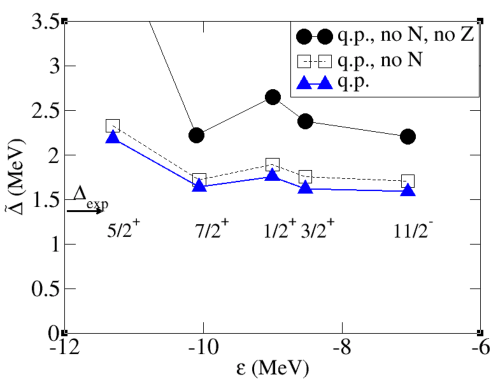
Figure 14: The pairing gaps obtained in the quasiparticle calculation (triangles) are compared to the results obtained neglecting the normalization factors $N$, and neglecting both $N$ and $Z$.

III.2 Comparison of prior and post scheme with the monopole pairing force

We have already noticed that solving the Nambu-Gor’kov equations in the post scheme is numerically very demanding in the case of realistic nucleon-nucleon interactions. In this Section we want to compare the prior and the post schemes using a simple monopole pairing force - $G_{0}P^{\dagger}P$ acting only in our valence space. The present calculation is similar to that presented in ref. Ter:02 , except for details in the mean field (here obtained from a SLy4 interaction instead of a Woods Saxon potential with effective mass $m^{*}$= 0.7), in the QRPA spectrum and in the determination of the PVC coupling. We shall however present new results which will extend our previous investigation.

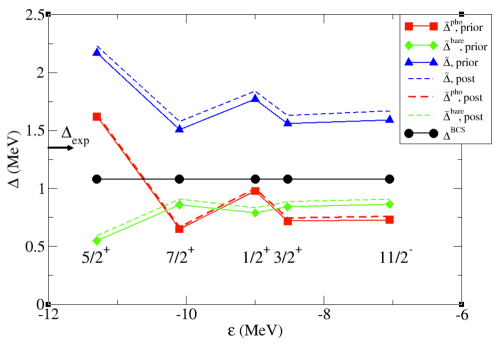
Figure 15: Comparison of the renormalized pairing gaps $\tilde{\Delta}$ associated with the lowest energy fragments, obtained solving the Nambu-Gor’kov equations in the prior (solid line with triangles) and in the post (dashed line) scheme. We also show the bare ($\tilde{\Delta}^{bare}$) and the phonon ($\tilde{\Delta}^{pho}$) components of the renormalized gaps in the prior (solid lines with diamonds and squares) and in the post (dashed lines) scheme. The pairing interaction is a monopole force with coupling constant $G_{0}=0.22$ MeV, acting in the valence shell around the Fermi energy in ¹²⁰Sn, which produces the gap $\Delta^{BCS}$ (solid lines with dots) obtained in the BCS calculation. The symbols refer to the position of the various valence orbitals in the SLy4 HF potential. The value of the gap $\Delta_{exp}$ obtained from the experimental odd-even mass difference is also indicated.

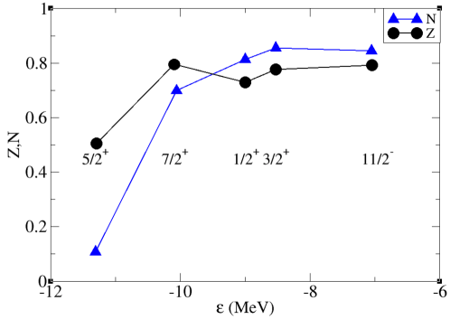
Figure 16: $Z-$ and $N-$factors associated with the various valence orbitals, for the calculation presented in Fig. 15. Prior and post values are indistinguishable at the scale of the figure.

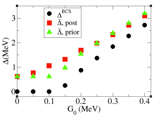
Figure 17: Renormalized gaps $\tilde{\Delta}$ obtained solving the Nambu Gor’kov equations in the prior and in the post scheme with the monopole pairing force as a function of the pairing constant $G_{0}$, averaged over the five valence orbitals. Also shown is the gap $\Delta^{BCS}$ obtained solving the BCS equation.

In Fig. 15 we compare the results obtained in the prior and in the post schemes, for a value $G_{0}$ = 0.22 MeV, corresponding to a bare pairing gap $\tilde{\Sigma}^{12bare}=$ 1.08 MeV. We have chosen this particular value of $G_{0}$ in order to reproduce the average value of the gap $\Delta^{BCS}$ obtained previously with the $v_{14}$ interaction (cf. Fig. 6). We see that the renormalized pairing gaps are very similar in the prior and post schemes. Moreover the results are also similar to those obtained with the Argonne interaction, shown in Fig. 6, not only for the total gap $\tilde{\Delta}$ but also concerning the decomposition into bare and phonon contribution. The similarity extends also to the $Z-$ and $N-$factors, shown in Fig. 16 (cf. Fig. 7). The fact that the results turn out to be close to those obtained using the Argonne interaction is easy to understand in the prior scheme, which is based on the quasiparticle and occupation amplitudes obtained with the bare interaction. In fact, the realistic nucleon-nucleon interaction displays a limited state dependence over the valence orbitals, with an average value $\Delta^{BCS}=1.1$ MeV, very close to the constant BCS gap obtained with the monopole interaction with $G_{0}=0.22$ MeV.

In Fig. 17 we show the value of the gap, averaged over the five valence orbitals, as a function of the pairing strength $G_{0}$. In the prior scheme, one starts from the $u_{a},v_{a}$ amplitudes obtained in a previous BCS calculation with the bare force, that for $G_{0}$ smaller than 0.1 MeV, produces no superfluid solution. On the other hand, the induced interaction $V_{ind}$ is able to produce a pairing gap by itself. As a consequence, in the prior scheme only $\tilde{\Sigma}^{12}_{phon}$ contributes to the gap, which is therefore underestimated and independent of $G_{0}$ for $G_{0}<0.1$. Instead, using the post scheme, the gap grows as a function of $G_{0}$ since the bare interaction can provide a contribution to pairing correlations even for small values of $G_{0}$ when it is added to the induced interaction through the effective interaction $V_{eff}=V_{bare}+V_{ind}$. For values of $G_{0}$ larger than 0.1 MeV, the gaps in the prior and post scheme become closer and closer, until the prior scheme becomes satisfactory for values of the order of $G_{0}$ = 0.2 MeV. It is interesting to notice that the calculations for the bare and renormalized gaps performed with $G_{0}=0.25$ MeV reproduce quite well the results obtained using the $V_{{\rm low}k}$ interaction as bare pairing force, as discussed in Section VI.2. This indicates that Fig. 17 can be used to assess in a simple way the effect of renormalization processes on pairing correlations, for the adopted QRPA spectrum.

IV Conclusions

We have presented a convenient formalism to deal with the basic renormalization processes induced by the coupling between quasiparticle and collecive vibrations in superfluid spherical nuclei. We have solved the Nambu-Gor’kov equations determining the normal and abnormal energy-dependent self-energies self-consistently. This allows a detailed calculation of the low-energy part of the nuclear spectrum in odd nuclei taking into account the fragmentation of the quasiparticle strength, as well as the calculation of the pairing gap of the system including the pairing interaction induced by the exchange of collective modes. The mean field is based on a Hartree-Fock calculation with the effective SLy4 interaction, while the coupling between quasiparticles and vibrations is determined by a QRPA calculation that reproduces the empirical polarizability of the low-lying vibrational modes. In the solution of Nambu-Gor’kov equations there are then no free parameters, when we use the bare $v_{14}$ Argonne nucleon-nucleon potential as bare pairing force. We have obtained a gap equation (cf. Eq. (59)) which takes into account renormalization effects in a compact way, and allows one to make contact with previous studies.

We have discussed in detail the practical implementation of the formalism, introducing two calculational schemes, depending on whether the bare pairing interaction and the renormalization effects are taken into account simultaneously (post scheme) or in two steps (prior scheme), performing first a BCS calculation with the bare force. We have shown that the two schemes lead to similar results for states close to Fermi energy in the case of a simple monopole pairing force with a realistic coupling strength. The prior scheme is computationally much simpler in the case of realistic nucleon-nucleon forces which can scatter particles to very high energies.

We have presented results for the semimagic nucleus ¹²⁰Sn, which are in rather good agreement with those extracted from one-neutron transfer reactions. The formalism allows also for a clear separation between the contribution of the bare force and of renormalization effects: their contributions to the pairing gap turn out to be of similar magnitude, confirming previous studies.

As we have already summarized in Section IV.1, we get an overall agreement with the experimental spectra. This agreement appears to be stable, respect to reasonable changes in the ingredients of our calculations (cf. the Appendix), and the contribution of the pairing interaction induced by surface vibration appears to be well established within our scheme.

Several elements remain to be further investigated, before one can reach firm quantitative theoretical results, in particular concerning the absolute value of the total pairing gap. On the one hand, the mean field should be either derived microscopically, or at least refitted comparing theory and experiment taking into account renormalization effects; on the other hand, contributions which are expected to provide a repulsive contribution to the pairing interaction, associated with three-body effects and with the influence of spin modes, have started only recently to be examined.

IV.1 Hindsight

One can conclude that it is possible, at least in the case of ¹²⁰Sn, to draw a picture that is consistent with the available experimental data concerning the quasiparticle properties close to Fermi energy. This is summarized in Fig. 18, which shows the results of a calculation with the bare pairing interaction, including all the elements discussed in the previous sections.

The spectroscopic factors and the induced pairing gap are not much affected by the details of the mean field or of the effective mass associated with the effective forces we have examined. These quantities are essentially determined by the interweaving with low-lying collective surface vibrations, which shifts the quasiparticle energies, increasing the level density close to the Fermi energy, and leads to spectroscopic factors ($Z-$ and $N-$ factors) in the range 0.6-0.8 (cf. Fig.18 (b)) and to an induced pairing gap $\Delta^{pho}$ of about 0.8 MeV. The coupling of spin modes, due to their higher energy and smaller collectivity, does not affect much the spectroscopic results. It reduces the induced pairing gap by about 0.2 MeV, leading to a final induced pairing gap $\Delta^{pho}$ close to 0.6 MeV (cf. Fig. 18 (a)).

The calculated strength function of fragmented levels (the $d_{5/2}$ in the present case) depends on the detailed position of the levels in the mean field potential, and the comparison with experiment provides important information on it. In the present case, we have explicitly verified that it is possible to reach a good overall agreement between theoretical and experimental spectra, both for the fragmented $5/2^{+}$ strength and for the other valence orbitals for which the quasiparticle approximation is valid, simply by adjusting the position of the $d_{5/2}$ orbital in the SLy4 HF potential (cf. Figs. 18 (c),(d)) .

We also find good agreement between the total pairing gap $\tilde{\Delta}$ and the value derived from the experimental odd-even mass difference, starting from the value $\Delta^{BCS}$ = 1.1 MeV obtained with the value of $m_{k}$ associated with the SLy4 interaction (cf. Fig. 18 (a)). In fact $\tilde{\Delta}=\tilde{\Delta}^{pho}+\Delta^{BCS}\times Z=$ 0.6 MeV + 0.8 MeV = 1.4 MeV.

We remark that microscopic pairing forces lead to a weak state dependence for the orbitals close to the Fermi energy, so that in this region we obtain essentially the same results - both at the BCS level and after the renormalization process - with a simple monopole interaction, using a suitable value of the pairing constant. Furthermore, different values of $\Delta^{BCS}$, associated with different momentum dependences of $m_{k}$ far from the Fermi energy, essentially lead to a shift of the final gap $\tilde{\Delta}$, but do not alter significantly the spectroscopic results shown in Fig. 18(b-d) (cf. Appendix VI.1).

Unfortunately, a conclusive theoretical calculation of $m_{k}$ is not yet available. Furthermore, one should add the effects of the three-body force, which is expected to lead to a repulsive contribution to the pairing interaction. Interestingly, a recent calculation of $\Delta^{BCS}$ using the $V_{{\rm low}k}$ pairing interaction and including three-body effects within the renormalization group approach, has produced a value for $\Delta^{BCS}$ close to 1.1 MeV in ¹²⁰Sn duguet_three ; duguet_threea .

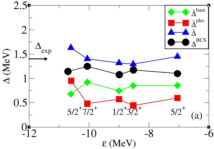
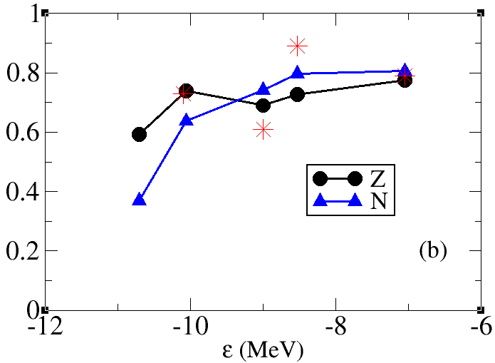
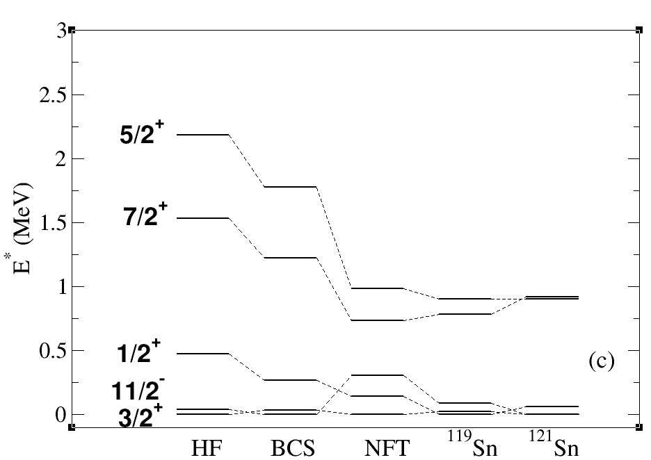
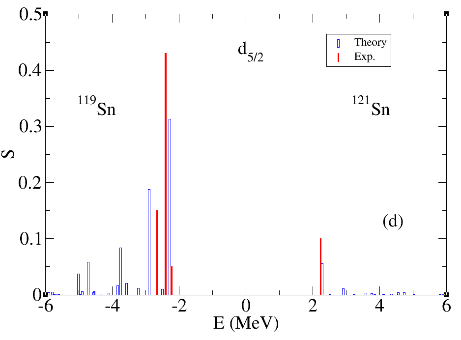
Figure 18: Results obtained solving the Nambu-Gor’kov equations including PVC to spin modes with the SLy4 mean field, shifting the energy of the $d_{5/2}$ orbital by 600 keV towards the Fermi energy: (a) renormalized gaps, (b) $Z$- and $N-$ factors, (c) quasiparticle spectrum, (d) $5/2^{+}$ strength function.

V Acknowledgment

Most of the work reported in this paper has been carried out in close collaboration with R.A. Broglia. F.B. acknowledges financial support from the Ministry of Science and Innovation of Spain grants FPA2009-07653 and ACI2009-1056.

VI Appendix

In this Appendix we consider the sensitivity of our results to some of the prescriptions and ingredients of the calculations.

VI.1 Mean field

Figure 19: Energies of the five HF single-particle levels lying close to the Fermi energy in ¹²⁰Sn, calculated with the effective interactions SKa, SLy4 and SGII. The effective mass associated with these forces at saturation density is also indicated.

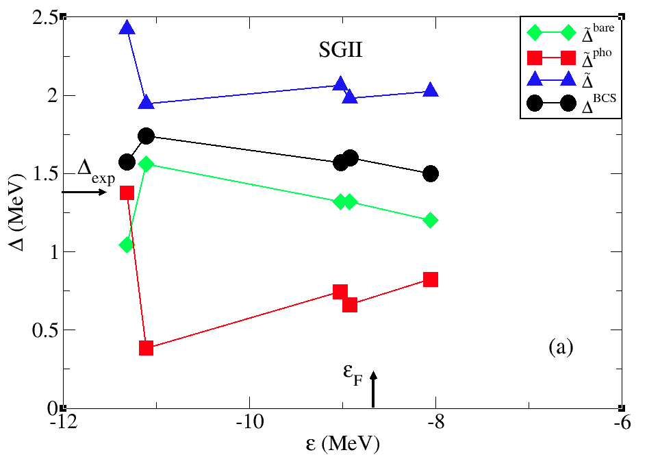
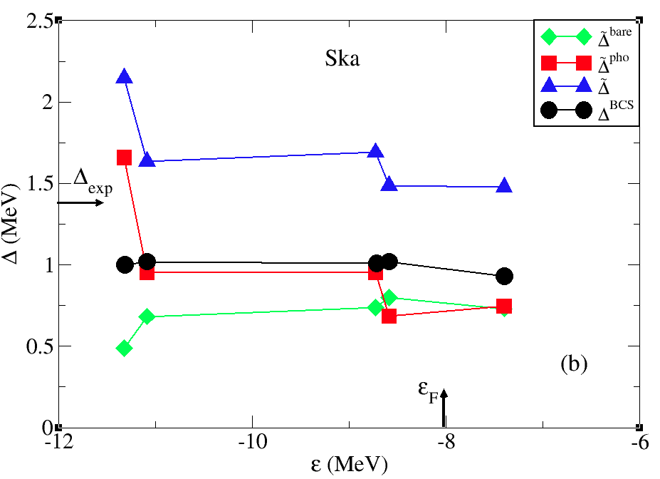
Figure 20: The state-dependent paring gap $\Delta^{BCS}$ calculated in BCS with the bare $v_{14}$ interaction is compared to the renormalized gap $\tilde{\Delta}$ (cf. Eq. (54) ) obtained solving the Nambu-Gor’kov equations. We compare results obtained with a mean field produced with the SGII interaction (a) and with the SKa interaction (b) (cf. Fig. 6 for the corresponding calculation with the SLy4 mean field) micene . The symbols refer to the position of the various valence orbitals in the SGII HF potential. We also show the decomposition of $\tilde{\Delta}$ into the bare and phonon contributions $\tilde{\Delta}^{bare}$ and $\tilde{\Delta}^{pho}$. The value of the Fermi energy $\epsilon_{F}$ and of the gap obtained from the experimental odd-even mass difference $\Delta_{exp}$ are also indicated.

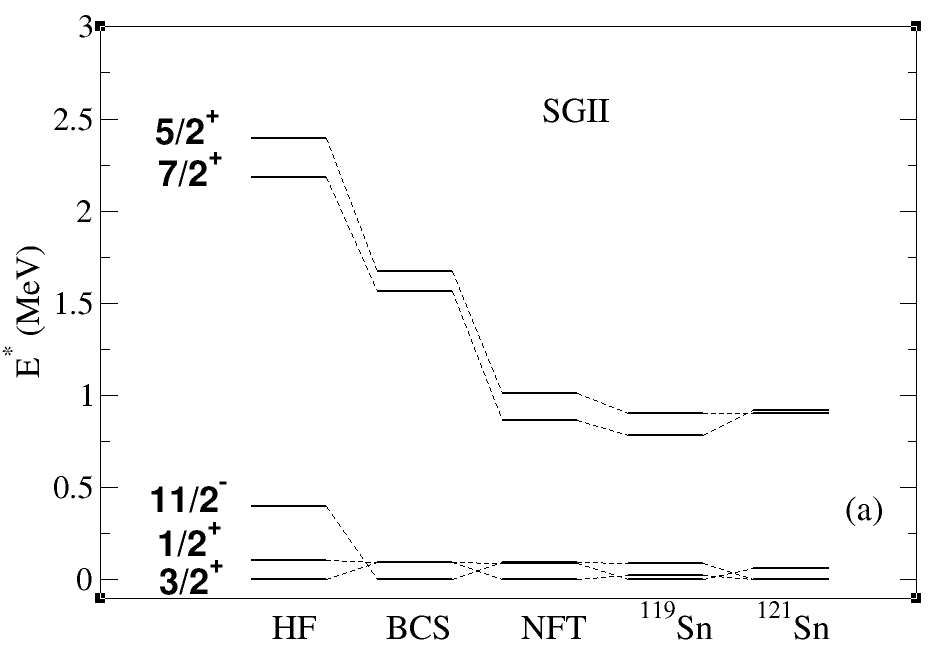
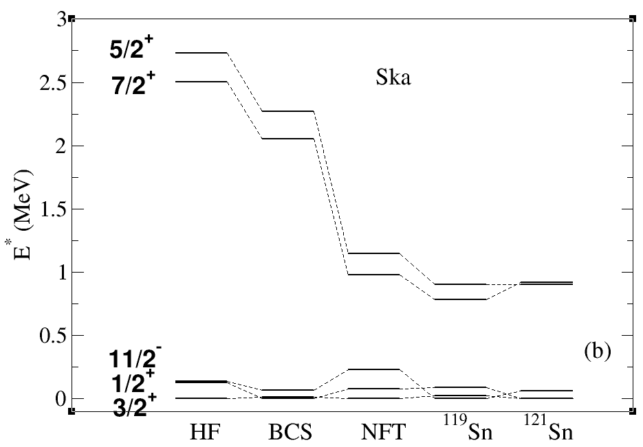
Figure 21: The theoretical quasiparticle spectra obtained at the various steps of the calculation are compared to the experimental data. We compare results obtained with a mean field produced with the SGII interaction (a) and with the SKa interaction (b) (cf. Fig. 8 for the corresponding calculation with the SLy4 mean field).

The results obtained in the main text have been obtained with a HF mean field produced by the SLy4 interaction, whose effective mass at saturation is $m_{k}=0.7m$. In this Section we show results obtained with two different interactions of the Skyrme type: the SKa kohler and the SGII sagawa , having respectively a lower ($m_{k}=0.61m$) and a larger ($m_{k}=0.78m$) effective mass. All the other features of the calculations are the same as for SLy4. In particular, the PVC matrix elements are the same, because in our approach they only depend on the properties of the phenomenological phonons and are calculated with the wavefunctions of a fixed potential with effective mass equal to one. As expected, the SGII interaction produces a mean field associated with a higher level density, leading to a larger pairing gap in the BCS calculation with the $v_{14}$ potential, as shown in Fig. 20(a): the value of $\Delta^{BCS}$ is equal to about 1.6 MeV, to be compared with the value 1.1 MeV previously obtained with the SLy4 interaction (cf. Fig. 6). The value obtained with the SKa interaction is instead equal to about 1 MeV (cf. Fig. 20(b)).

The renormalization processes act in a very similar way as was previously found in the case of SLy4. The average value of the phonon induced gap $\Delta^{pho}$ is in all cases equal to about 0.8 MeV: in the case of SGII $\Delta^{pho}$ accounts for about 30% of the total gap, while in the case of SKa $\Delta^{pho}$ and $\Delta^{bare}$ are of similar magnitude, as in the case of SLy4.

The low-lying spectra are shown in Fig. 21, while the $Z-$ and $N-$factors of the lowest fragments are reported in Fig. 23. Also in this case, the action of the PVC is similar to that already discussed in the case of the SLy4 interaction (cf. Fig. 8). However, the agreement with experiment is better than obtained previously. This is due to the initial position of the $d_{5/2}$ and $g_{7/2}$ orbitals, which are closer to each other; furthermore, the $d_{5/2}$ single-particle calculated with SGII lies at a distance of about 2.2 MeV from the Fermi energy, instead of 2.8 MeV as in the case of SLy4: this leads to a good description of the fragmentation of this orbital, as shown in Fig. 22, that in the case of SLy4 was obtained only shifting the energy of this level (cf. Figs. 10 and 18). The quality of the spectrum obtained with SKa is almost as good as with SGII: however, the orbital $g_{7/2}$ lies more distant from the Fermi energy and becomes fragmented, contrary to experiment (cf. Fig. 23). It is interesting to notice that taking the SLy4 mean field, and changing the energies of the five valence orbitals with those associated with the SGII interaction, one obtains practically the same spectrum and the same $Z-$ and $N-$ factors as with SGII. This in spite of the fact that $\Delta^{BCS}$ becomes equal to about 1.25 MeV, to be compared with 1.1 MeV (SLy4) and 1.6 MeV (SGII). At the same time, the average value of $\tilde{\Delta}$ is equal to about 1.7 MeV, to be compared with 1.6 MeV (SLy4) and 2.1 MeV (SGII) (cf. Fig. 24). These results show that the low-energy spectrum is determined by the position of the valence orbitals, while the absolute value of the BCS gap also depends on the effective mass associated with distant levels.

We can conclude that renormalization effects are similar for the three mean fields we have considered. The comparison with the odd-even mass difference favours forces having low effective mass (SLy4 or SKa). The PVC improves the agreement of the spectral properties with experiment. However, the quality of this agreement depends on the specific position of the mean field single-particle levels close to the Fermi energy. The value of the effective mass far from the Fermi energy determines the magnitude of the final gap $\tilde{\Delta}$ by shifting the value of $\Delta^{BCS}$, while the value of $\Delta^{pho}$ and the properties of the low-lying spectrum are not very sensitive to it.

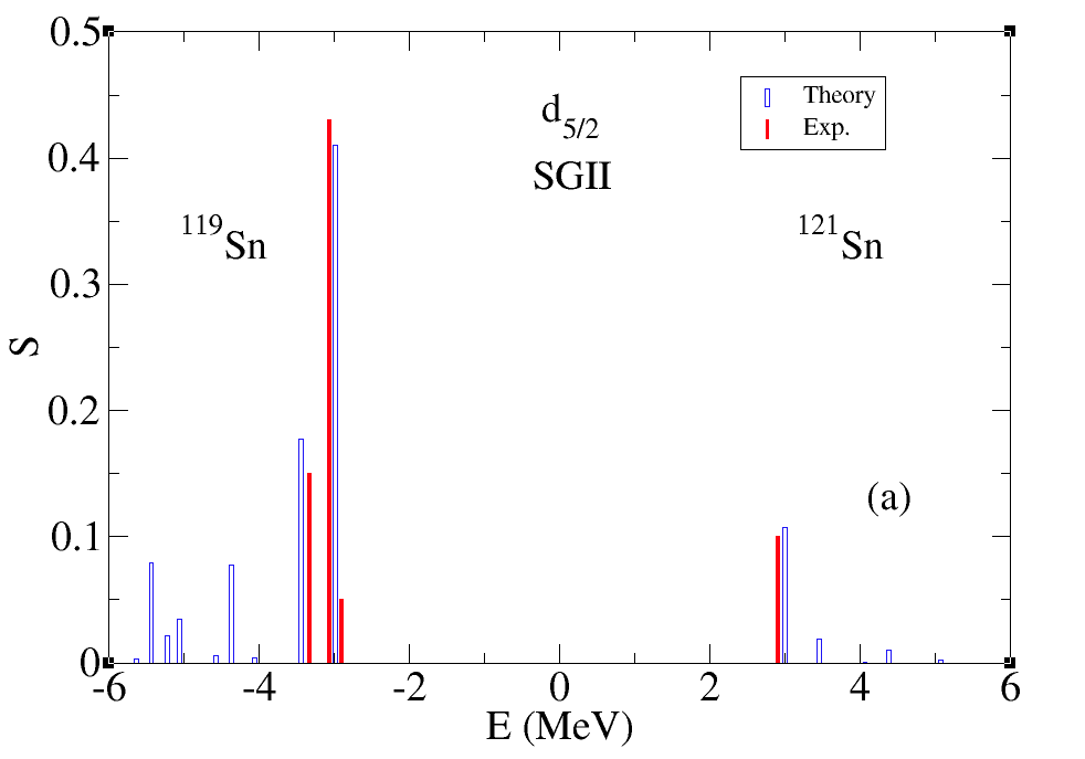
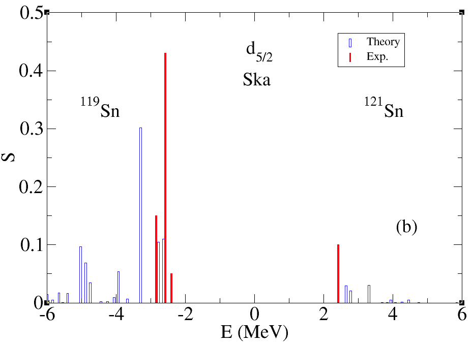
Figure 22: The theoretical strength function calculated for the $d_{5/2}$ orbital is compared to the spectroscopic factors associated with experimental levels detected in one-neutron transfer reactions. We compare results obtained with a mean field produced with the SGII interaction (a) and with the SKa interaction (b) (cf. Fig. 10 for the corresponding calculation with the SLy4 mean field).

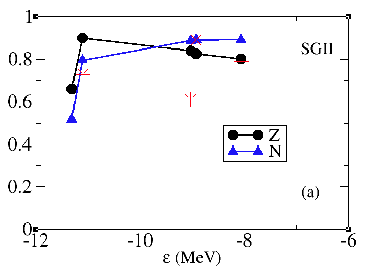
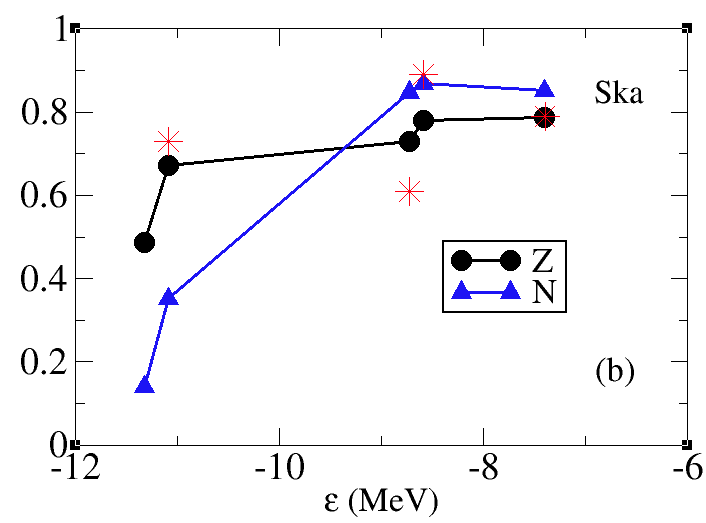
Figure 23: Comparison of the $N-$ and $Z-$ factors associated with the lowest quasiparticle peaks in the Nambu-Gor’kov calculation shown in Fig. 20. We compare results obtained with a mean field produced with the SGII interaction (a) and with the SKa interaction (b) (cf. Fig. 7 for the corresponden calculation with the SLy4 mean field). Also shown by stars are the values of the experimental quasiparticle strength exp_transf2 , except for the $d_{5/2}$ orbital which shows a pronounced fragmentation.

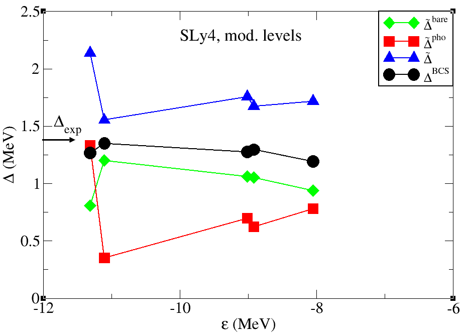
Figure 24: The same as in Fig. 20, for the pairing gaps calculated with the SGII mean field, but substituting the single-particle energies of the five valence orbitals with the energies calculated in the SLy4 mean field.

VI.2 Bare pairing interaction

The calculations reported in the main text have been carried out adopting $v_{14}$ as the bare pairing force. However, the $V_{{\rm low}k}$ version of the Argonne potential has been used by several groups and here we show the results using this bare pairing force in our Nambu-Gor’kov formalism. The corresponding bare and renormalized gap are shown in Fig. 25. The average value of the bare gap is equal to about 1.4 MeV, in agreement with ref. hebeler , to be compared with the value 1.1 MeV obtained with the Argonne interaction. The effect of the renormalization processes increases the gap on average by about 500 keV, similar to the case of $v_{14}$ (600 keV, cf. Fig. 6). Also the values of the phonon induced component $\Delta^{pho}$ are quite similar. The results of the calculations with $v_{14}$ and $V_{{\rm low}k}$ turn out to be quite similar to those obtained in Section III using the monopole force respectively with coupling constants $G_{0}=0.22$ and $G_{0}=0.25$ MeV (cf. Fig. 17).

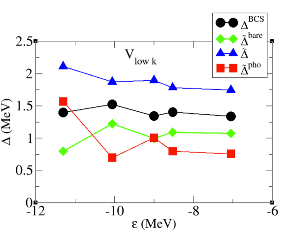
Figure 25: The state-dependent paring gap $\Delta^{BCS}$ calculated using the $V_{{\rm low}k}$ potential with a cutoff $\Lambda=4$ fm^-1 as pairing force is compared to the renormalized gap $\tilde{\Delta}$ (cf. Eq. (54) ) obtained solving the Nambu-Gor’kov equations. The symbols refer to the position of the various valence orbitals in the SLy4 HF potential. We also show the decomposition of $\tilde{\Delta}$ into the bare and phonon contributions $\tilde{\Delta}^{bare}$ and $\tilde{\Delta}^{pho}$. We thank A. Pastore for providing us with the HFB calculation with the $V_{{\rm low}k}$ potential.

VI.3 QRPA

We recall (cf. Section II) that the results shown in the main text are based on effective PVC vertices calculated with single-particle levels and wavefunction associated with a Woods-Saxon potential, with an associated effective mass $m^{*}=m$. Another reasonable choice, often adopted in the literature, would be to use instead the same single-particle levels used in the HF+BCS calculation. Using this prescription and readjusting the coupling constants $\chi_{\lambda}$ of the QRPA calculation so as to reproduce the experimental properties of the low-lying vibrational states, we obtain the renormalized pairing gaps shown in Fig. 26. It is seen that the difference is not critical, our preferred choice leading to gaps which are smaller by about 10%.

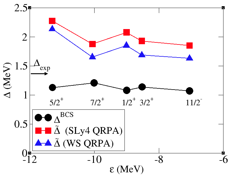
Figure 26: The renormalized pairing gaps $\tilde{\Delta}$, calculated using the levels of a Woods-Saxon potential to compute the QRPA spectrum and the PVC vertices, are shown by triangles (cf. Fig. 6) and are compared to the results obtained using SLy4 single-particle levels (squares). We also show by dots the pairing gap $\Delta^{BCS}$ calculated in BCS.

VI.4 Bubble approximation

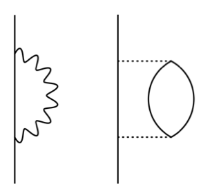
Figure 27: While in the rest of the work we have considered the effect of the coupling betwene quaisparticle and collective QRPA phonons (left), in this section we shall consider the coupling to uncorrelated excitations (right).

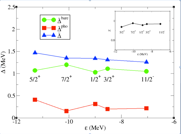
Figure 28: Pairing gaps associated with the main quasiparticle peaks obtained in the one-bubble approximation. We show the total renormalized gap $\tilde{\Delta}$ and its decomposition into the bare and the phonon contributions. In the inset, the $Z-$values are also shown.

It is interesting to assess the importance of the collectivity of QRPA modes in the pairing calculation. This can be done by comparing our previous results with calculations performed coupling the quasiparticles with unperturbed p-h excitations (cf. Fig. 27). In Fig. 28 we show the pairing gap and the $Z-$ factors calculated at the p-h level: they are very close to 1, indicating that the renormalization processes are much less important as compared to the calculations with collective modes. Correspondingly, the phonon contribution to the gaps is drastically diminished (compare with Figs. 6 and 7 ). Also the quasiparticle spectrum becomes very close to that obtained at the HF+BCS level. On the other hand, the total gap is reduced by only 10% as compared to the QRPA result: this happens because, even if the phonon-induced interaction is considerably weaker, the product $\tilde{\Delta}=Z\Delta^{BCS}+\tilde{\Delta}^{pho}$ is much less affected, because the $Z-$factor is correspondingly increased. Schematically, while in the QRPA case one finds $Z\approx 0.75$ and $\tilde{\Delta}=0.75\times 1.1+0.8$ = 1.6 MeV, in the present case $Z\approx 0.95$ and $\tilde{\Delta}=0.95\times 1.1+0.3$ = 1.4 MeV. One then concludes that, although the value of the gap is similar using the QRPA or the unperturbed response, the physical picture is quite different. This is related to the fact that the contribution of the phonon interaction to the total gap is equal to about 50% considering the coupling to QRPA modes, and to about 20% coupling to unperturbed p-h excitations. Furthermore, we have performed a calculation correcting for the Pauli principle, namely removing the contribution from a bubble when the particle or the hole coincides with the intermediate state $\{nlj\}$, with the proper angular momentum factor $1/(2j+1)$ (cf. broglia_brink , Appendix F). The pairing gap is reduced by less than 5%. This represents an upper limit for role of the Pauli correction in the calculations based on collective phonons reported in the main text.

References

- (1) C. Mahaux, P.F. Bortignon, R.A. Broglia and C.H. Dasso, Phys. Rep. 120 (1985) 1
- (2) V.G. Soloviev, Theory of atomic nuclei. Quasiparticles and nuclei, Instit=tute of Physics Publishing, Bristol-Philadelphia (1992)
- (3) L.P. Gor’kov, Sov. Phys. JETP 7 (1958) 505
- (4) Y. Nambu, Phys. Rev. 117 (1960) 648
- (5) G.M. Eliashberg, Sov. Phys. JETP 11 (1960) 696
- (6) G. Potel, A. Idini, F. Barranco, E. Vigezzi and R.A. Broglia, nucl-th/0906.4298
- (7) F. Barranco, R.A. Broglia, G. Gori, E. Vigezzi, P.F. Bortignon and J. Terasaki, Phys. Rev. Lett. 83 (1999) 2147
- (8) J. Terasaki, F. Barranco, R.A. Broglia, E. Vigezzi and P.F. Bortignon, Nucl. Phys. A 697 (2002) 127
- (9) J. Terasaki, F. Barranco, R.A. Broglia, E. Vigezzi and P.F. Bortignon, Progr. Theor. Phys. 108 (2002) 495
- (10) F. Barranco, R.A. Broglia, G. Colò, E. Vigezzi and P.F. Bortignon, Eur. Phys. Jou. A 21 (2004) 57
- (11) F. Barranco, P.F. Bortignon, R.A. Broglia, G. Colò, P. Schuck, E. Vigezzi and X. Viñas, Phys. Rev. C72 (2005) 054314
- (12) A. Pastore, F. Barranco, R.A.Broglia and E. Vigezzi, Phys. Rev. C 78 (2008) 024315
- (13) D.R. Bes, R.A. Broglia, G.G. Dussel, R.J. Liotta and R.J. Perazzo, Nucl. Phys. A 260 (1976) 1
- (14) P.F. Bortignon, R.A. Broglia, D.R. Bes and R. Liotta, Phys. Rep. 30C 1977 305
- (15) A. Bohr and B.R. Mottelson, Nuclear Structure, Vol. II, Benjamin (1975)
- (16) P.F. Bortignon and R.A. Broglia, Nucl. Phys. A 371 (1981) 405
- (17) R.A. Broglia, F. Barranco, G. Colò, G. Gori and E. Vigezzi, in Proc. of the International School of Physics ”Enrico Fermi”, Course CLIII, A. Molinari, L. Riccati, W.M. Alberico and M. Morando eds., p. 65
- (18) C. Barbieri and W.H. Dickhoff, Phys. Rev. C 65 064313 (2002)
- (19) C. Barbieri and W.H. Dickhoff, Phys. Rev. C 68 014311 (2003)
- (20) C. Barbieri and M. Hjorth-Jensen, Phys. Rev C 79 (2009) 064313
- (21) G. Colò, H. Sagawa and P.F. Bortignon, Phys. Rev. C 82 (2010) 064307
- (22) A. Ansari and P. Ring, Phys. Rev. C 74 (2006) 054313
- (23) J. Terasaki, J. Engel and G.F. Bertsch, Phys. rev. C78 (2008) 044311
- (24) W.H. Dickhoff and D. Van Neck, Many-Body theory exposed! Propagator description of quantum mechanics in many-body systems, World Scientific, 2nd Edition (2008)
- (25) V. Van der Sluys, D. Van Neck, M. Waroquier and J. Ryckebusch, Nucl. Phys. A 551 (1993) 210
- (26) J.R. Schrieffer, Superconductivity, Benjamin (1964)
- (27) R.A. Broglia, O. Hansen and C. Riedel, Ed. M. Baranger and E. Vogt, Plenum Press, Vol.6, 287 (1973)
- (28) A. Bohr and B.R. Mottelson, Nuclear Structure, Vol. I, Benjamin (1969)
- (29) D. Rowe, Nuclear collective motion, Methuen (1970)
- (30) C. Bloch and Horowitz, Nucl. Phys. 8 (1958) 91
- (31) S.T. Belyaev and V.G. Zelevinskii, Sov. J. Nucl. Phys. 1 (1965) 10
- (32) A.V. Avdeenkov and S.P. Kamerdzhiev, in Proc. of the 7th Int. Spring Seminar on Nuclear Physics, Challenges of nuclear structure, Maiori 2001, nucl-th/0111072
- (33) D.R. Bes, R.A. Broglia, G.G. Dussel, R.J. Liotta and H.M. Sofia, Nucl. Phys. A 260 (1976) 27
- (34) A.V. Avdeenkov and S.P. Kamerdzhiev, Phys. At. Nucl. 62 (1999) 563
- (35) A.V. Avdeenkov and S.P. Kamerdzhiev, Phys. Lett. B 459 (1999) 423
- (36) V.A. Khodel, Phys. Rep. 92 (1983) 183
- (37) F. Barranco and R.A. Broglia, Phys. Rev. Lett. 59 (1987) 2724
- (38) V.A. Khodel, A.P. Platonov and E.E. Saperstein J. Phys. G 8 967 (1982)
- (39) S.A. Fayans, S.V. Tolokonnikov, E.L. Trykov and D. Zawischa, Nucl. Phys. A 676 (2000) 49
- (40) F. Barranco and R.A. Broglia, Phys. Lett. B 151 (1985) 90
- (41) J.I. Escudero, F. Barranco and G. Madurga, J. Phys. G. 13 1261 (1987)
- (42) S. Kamerdzhiev and E.E. Saperstein, Eur. Phys. Jou. 333 (2008) 37
- (43) F. Barranco, P.F. Bortignon, R.A. Broglia, G. Colò and E. Vigezzi, Eur. Phys. Jou. A 11 (2001) 385
- (44) G. Gori, F. Barranco, E. Vigezzi and R.A. Broglia, Phys. Rev. C 69 (2004) 041302(R)
- (45) U. Lombardo, P. Schuck and W. Zuo, Phys. Rev. C 64 (2001) 021301(R)
- (46) M. Baldo and A. Grasso, Phys. Lett. B 485 (2000) 115
- (47) S. Baroni, A.O. Macchiavelli and A. Schwenk, Phys. Rev. C 81 (2010) 064308
- (48) D. Van Neck, M. Waroquier and J. Ryckebusch, Nucl. Phys. A 530 (1991) 347
- (49) D. Van Neck, M. Waroquier, V. Van der Sluys and J. Ryckebusch, Nucl. Phys. A 563 (1993) 1
- (50) O. Beer, A. El Behay, P. Lopato, Y. Terrien, G. Vallois and Kamal K. Seth, Nucl. Phys. A 147 (1970) 326
- (51) F. Barranco, R.A. Broglia, H. Esbensen and E. Vigezzi, Phys. Lett. B 390 (1996) 13
- (52) P.M. Pizzochero, F. Barranco, E. Vigezzi and R.A. Broglia, APJ 569 (2002) 381
- (53) P. ring and P. Schuck, The nuclear many-body problem, Springer-Verlag, New York (1980)
- (54) E. Chabanat, P. Bonche, P. Haensel, J. Meyer and R. Schaeffer, Nucl. Phys. A 635 (1998) 231
- (55) T. Lesinski, M. Bender, K. Bennaceur, T.Duguet and J. Meyer, Phys. Rev. C 76 (2007) 014302
- (56) G. Colò, S. Fracasso and P.F. Bortignon, Phys. Lett. B 646 (2007) 227
- (57) K. Hebeler, T. Duguet, T. Lesinski and A. Schwenk, Phys. Rev. C 80 (2009) 044321
- (58) M. Baldo, U. Lombardo, S.S. Pankratov and E.E. Saperstein, J. Phys. G 37 (2010) 064016
- (59) W. Zuo, U. Lombardo, H.-J. Schulze and C.W. Shen, Phys. Rev C 66 (2002) 037303
- (60) T. Duguet, T. Lesinski, K. Hebeler and A. Schwenk, Mod. Phys. Lett. 25 (2010) 1989
- (61) T. Duguet, T. Lesinski, K. Hebeler and A. Schwenk, nucl-th/1104.2955
- (62) M. Bender, K. Rutz, P.-G. Reinhard and J.A. Maruhn, Eur. Phys. J. A 8 (2000) 49
- (63) T. Duguet, P. Bonche, P.-H. Heenen and J. Meyer, Phys. Rev. C 65 (2001) 014311
- (64) F. Barranco, R.A. Broglia, H. Esbensen, E. Vigezzi, Phys. Lett. B 390 (1997) 13
- (65) E. Gerlic, G. Berrier-Ronsin, G. Duhamel, S. Galès, E. Hourani, H. Langevin-Joliot, M. Vergnes, and J. Van de Wiele, Phys. Rev. C 21 (1980) 124
- (66) S.A. Dickey, J.J. Kraushaar, R. Ristinen and M.A. Rumore, Nucl. Phys. A 377 (1982) 137
- (67) M. J. Bechara and O. Dietzch, Phys. Rev. 12 (1975) 90
- (68) K. Moghrabi, M. Grasso, G. Colò and N. Van Giai, Phys. Rev. Lett. 105 (2010) 262501
- (69) J. M. C. Chen, J. W. Clark, R. D. Davé and V. V. Khodel, Nucl. Phys. A 555 (1993) 59
- (70) J. Wambach, T. Ainsworth and D. Pines, Nucl. Phys. A 555 (1993) 128
- (71) H.-J. Schulze, J. Cugnon, A. Lejeune, M. Baldo, and U. Lombardo, Phys. Lett. B 375 (1996) 1
- (72) H. Heiselberg, C.J. Pethick, H. Smith and L. Viverit, Phys. Rev. Lett. 85 (2000) 2418
- (73) G. Gori, F. Barranco, R.A. Broglia, G. Colò, E. Vigezzi and P.F. Bortignon, Phys. Rev. C 72 011302 (2005)
- (74) D.M. Brink and R.A. Broglia, Nuclear Superfluidity, Cambridge University Press, Cambridge (2005).
- (75) L. Micene, Mater Thesis, University of Milano (2007), unpublished.
- (76) H. Köhler, Nucl. Phys. A 258 301 (1976)
- (77) N. van Giai and H. Sagawa, Phys. Lett. B 106 (1981) 379