Optimized hierarchical equations of motion for Drude dissipation

Abstract

The hierarchical equations of motion theory for Drude dissipation is optimized, with a convenient convergence criterion proposed in advance of numerical propagations. The theoretical construction is on basis of a Padé spectrum decomposition that has been qualified to be the best sum-over-poles scheme for quantum distribution function. The resulting hierarchical dynamics under the apriori convergence criterion are exemplified with a benchmark spin-boson system, and also the transient absorption and two-dimensional spectroscopy of a model exciton dimer system.

I Introduction

Quantum dissipation plays a pivotal role in many chemical, physical, and biological problems.Nit06 ; Wei08 ; Kle09 ; Yan05187 Recent experiments on excitation energy transfer in photosynthesis systemsEng07782 ; Col10644 show clearly the breakdown of conventional Markovian and perturbative quantum dissipation theories.Ish09234110 ; Ish09234111 The protein environment is nano-structured, with the time scale of modulation comparable to that of the excitation energy transfer. Also the protein-pigment coupling strength is about that between pigments. Apparently, one needs a nonperturbative, non-Markovian, and also numerically implementable quantum dissipation theory. The demand is the same on the study of heating generation in quantum transport through mesoscopic systemsSeg023915 ; Gal081056 ; Pop10147 and protection of qubits with the aid of photonic crystal environment.Lod04654 ; Sap101352 ; Wol10141108

This work focuses on the hierarchical equations of motion (HEOM) approach.Tan906676 ; Ish053131 ; Tan06082001 ; Yan04216 ; Xu05041103 ; Xu07031107 We request the best HEOM construction, exemplified with Drude dissipation, together with a convenient criterion to estimate its convergency before propagations for general systems at any finite temperature. HEOM approach was originally proposed in 1989 by Tanimura and Kubo for semiclassical dissipation.Tan89101 Formally exact HEOM formalismTan906676 ; Ish053131 ; Tan06082001 ; Yan04216 ; Xu05041103 ; Xu07031107 for Gaussian dissipation in general, including its second quantization,Jin08234703 is now well established, with the aid of proper environment spectrum decomposition schemes. As a numerically efficient alternative to path integral influence functional,Fey63118 ; Wei08 ; Kle09 HEOM has been applied to such as electron transfer,Shi09164518 ; Xu09214111 ; Tia10114112 ; Tia10114112note ; Tan10214502 nonlinear optical spectroscopy,Ish06084501 ; Ish079269 ; Tan091270 ; Che10024505 ; Che11194508 ; Zhu115678 and transient quantum transport.Zhe08184112 ; Zhe08093016 ; Zhe09164708

To have an explicit HEOM construction one should exploit certain basis set spanning over the stochastic bath space. This is equivalent to the choice of certain sum-over-pole (SOP) scheme that decomposes individual bath correlation function into its multiple-timescale memory spectrum components. The conventional scheme is the Matsubara expansion of quantum distribution function (i.e., the Bose/Fermi function) involved in the bath correlation functions. Wei08 ; Kle09 ; Yan05187 However, Matsubara expansion is notorious for slow convergence. We have recently proposed three Padé spectrum decomposition (PSD) schemesHu10101106 ; Hu11jcp be the candidates for the best SOP method. Mathematically, these three PSDs of Bose/Fermi function exploit the $[N\!-\!1/N]$, $[N/N]$, and $[N\!+\!1/N]$ Padé approximants, respectively. The resulting HEOM dynamics have been demonstrated in context of transient quantum transport through a double quantum dots system and population transfer in a spin-boson system.Hu11jcp

Three closely related issues arise in the choice of statistical environment basis set (or SOP scheme) for efficient HEOM construction. The first one is to identify the best basis set for spanning over the stochastic bath space. The second one concerns the minimum basis set. It requests to have not only the smallest number of decomposition terms, but also a priori accuracy control criterion on the resulting HEOM dynamics for any given system under bath influence at finite temperature. The third issue is about the possibility of at least partial inclusion of the off-basis-set residue effect on the HEOM dynamics.

In this work, we construct an optimized HEOM theory for Drude dissipation. We identity that $[N/N]$ PSD serves as the best and the minimum Drude dissipation basis set. It leads naturally to an off–basis–set white noise residue (WNR) term, together with a simple accuracy control criterion on the resulting HEOM dynamics. The present paper is a generalization of Ref. Xu09214111, and Ref. Tia10114112, , where $N=0$ and $N=1$ cases were analyzed, respectively. We summarize the PSD-based HEOM formalism with the Drude bath in Sec. II, followed by proposing the accuracy control criterion. Numerical demonstrations are carried out in Sec. III. Included there are a benchmark spin-boson dynamics, studied before by Thoss, Wang, and Miller,Tho012991 and the nonlinear optical signals of a model dimer system. Finally we conclude the paper in Sec. IV.

II Formalism

II.1 Optimal hierarchy for Drude dissipation

In this subsection, we exploit the $[N/N]$ PSD schemeHu11jcp to construct HEOM for Drude dissipation cases. HEOM has the following generic form,Xu07031107

$$\dot{\rho}_{{\sf n}}(t)=-[i{\cal L}(t)+\gamma_{{\sf n}}+\delta{\cal R}_{\sf n}]\rho_{{\sf n}}(t)+\rho_{\sf n}^{{}_{\{\!-\!\}}}(t)+\rho_{\sf n}^{{}_{\{\!+\!\}}}(t).$$ (1)

It describes how an $n^{\rm th}$-tier ADO $\rho_{\sf n}$ depends on its associated $(n\pm 1)^{\rm th}$-tier ADOs in $\rho_{\sf n}^{{}_{\{\!\pm\!\}}}$. The ADO’s index ${\sf n}$ is in general a collection of indices; i.e., ${\sf n}\equiv\{n_{1},\cdots,n_{K}\}$, with $n_{k}\geq 0$ for bosonic bath. Here $n_{1}+\cdots+n_{K}=n$ for $\rho_{\sf n}=\rho_{n_{1},\cdots,n_{K}}$ being called an $n^{\rm th}$-tier ADO. The reduced system density operator $\rho(t)\equiv{\rm tr}_{\mbox{\tiny B}}\rho_{\rm total}(t)\equiv\rho_{\sf 0}(t)$ is just the zeroth-tier ADO. In Eq. (1), the reduced system Liouvillian ${\cal L}(t)\,\cdot\,\equiv[H(t),\,\cdot\,]$ can be time dependent, e.g., in the presence of driving fields. Throughout of this paper, we set $\hbar=1$ and $\beta=1/(k_{B}T)$, with $k_{B}$ being the Boltzmann constant and $T$ the temperature.

The specific HEOM construction, including the ADO labeling index ${\sf n}=\{n_{1},\cdots,n_{K}\}$, depends on the way of decomposing bath correlation function into its memory spectrum components. For clarity, let the system-bath interaction be $H^{\prime}(t)=-{\hat{Q}}{\hat{F}}_{\mbox{\tiny B}}(t)$, with $\hat{Q}$ and $\hat{F}_{\mbox{\tiny B}}(t)$ being operators in the reduced system and the stochastic bath subspaces, respectively. The influence of bath on system is completely determined by the correlation function $C(t)\equiv\langle\hat{F}_{\mbox{\tiny B}}(t)\hat{F}_{\mbox{\tiny B}}(0)\rangle_{\mbox{\tiny B}}$. It is in turn related to the bath spectral density $J(\omega)$ via the fluctuation-dissipation theorem (FDT):Wei08 ; Kle09 ; Yan05187

$$C(t)=\frac{1}{\pi}\int_{-\infty}^{\infty}\!\!d\omega\frac{e^{-i\omega t}J(\omega)}{1-e^{-\beta\omega}}.$$ (2)

To have a HEOM construction,Xu07031107 we expand $C(t)$ in a finite exponential series, on the basis of certain SOP scheme, together with the Cauchy residue theorem of contour integration.

In this work we focus on the Drude model,

$$J(\omega)=\frac{2\lambda\gamma\omega}{\omega^{2}+\gamma^{2}}.$$ (3)

It has only one pole, $z=-i\gamma\equiv-i\gamma_{\mbox{\tiny D}}$, in the lower-half plane. The exponential series of bath correlation function assumes then

$$C(t)=\sum_{k={\rm D},1}^{N}\!\!c_{k}e^{-\gamma_{k}t}+\delta C_{N}(t).$$ (4)

In general the off-basis-set residue $\delta C_{N}(t)\neq 0$, as one exploits only finite $N$ poles for Bose function. The conventional scheme is the Matsubara expansion which is however notorious for slow convergence.Wei08 ; Kle09 For Drude dissipation it has been suggestedTia10114112 that $[N/N]$ PSD be the best SOP of Bose function. It is accurate up to ${\cal O}(x^{4N+1})$ in the order of $x=\beta\omega$ and reads Hu11jcp

$$\frac{1}{1-e^{-x}}\approx f^{[N/N]}(x)=\frac{1}{x}+\frac{1}{2}+\sum_{k=1}^{N}\frac{2\eta_{k}x}{x^{2}+\xi^{2}_{k}}+R_{N}x,$$ (5)

with

$$R_{N}=\frac{1}{4(N+1)(2N+3)}\,.$$ (6)

The PSD poles and coefficients, $\{\xi_{k},\eta_{k};k=1,\cdots,N\}$, are all positive and can be evaluated with high precision via the eigenvalues of real symmetric triangle matrices.Hu11jcp

The corresponding exponential series expansion of Eq. (4) can now be obtained via the standard contour integration technique. We obtain (setting $\gamma_{k}\equiv\xi_{k}/\beta$)

$$\begin{split}&c_{\mbox{\tiny D}}=-2i\lambda\gamma f^{[N/N]}(\beta z)\big{|}_{z=-i\gamma},\\ &c_{k}=\frac{2\eta_{k}}{i\beta}J(z)\big{|}_{z=-i\gamma_{k}};\ k=1,\cdots,N,\end{split}$$ (7)

and

$$\delta C_{N}(t)\approx 4\lambda\beta\gamma R_{N}\delta(t)\equiv 2\Delta_{N}\delta(t).$$ (8)

Note that $\{c_{k};k=1,\cdots,N\}$ are all real. On the other hand, $c_{\mbox{\tiny D}}$ associating with the Drude exponent $\gamma_{\mbox{\tiny D}}=\gamma$ is complex and is evaluated by using the $[N/N]$ Bose function $f^{[N/N]}(x)$, as given by the last expression of Eq. (5).

The SOP scheme resembles a statistical environment basis set for the HEOM construction. It dictates not only the exponential expansion of $C(t)$ as Eq. (4), but also HEOM. The ADO reads now $\rho_{\sf n}\equiv\rho_{n_{\mbox{\tiny D}},n_{1},\cdots,n_{N}}$. The only approximation involved is the WNR treatment of the off-basis-set $\delta C_{N}(t)$ by Eq. (8). It results in the WNR of $\delta{\cal R}_{{\sf n}}$ in Eq. (1) without further approximation:Ish053131 ; Xu07031107

$$\delta{\cal R}_{{\sf n}}\rho_{{\sf n}}=\Delta_{N}[\hat{Q},[\hat{Q},\rho_{{\sf n}}]].$$ (9)

The damping parameter in Eq. (1) collects all relevant exponents:Xu07031107

$$\gamma_{{\sf n}}=\sum_{k={\rm D},1}^{N}n_{k}\gamma_{k}.$$ (10)

The tier-down and tier-up terms are Xu07031107 ; Shi09084105

$$\begin{split}\rho_{\sf n}^{{}_{\{\!+\!\}}}&=-i\sum_{k={\rm D},1}^{N}\sqrt{(n_{k}+1)|c_{k}|}\,\bigl{[}\hat{Q},\rho_{{{\sf n}}_{k}^{+}}\bigr{]}\,,\\ \rho_{\sf n}^{{}_{\{\!-\!\}}}&=-i\sum_{k={\rm D},1}^{N}\sqrt{\frac{n_{k}}{|c_{k}|}}\,\bigl{(}c_{k}\hat{Q}\rho_{{{\sf n}}_{k}^{-}}-c^{\ast}_{k}\rho_{{{\sf n}}_{k}^{-}}\hat{Q}\bigr{)}\,,\end{split}$$ (11)

with $\rho_{{{\sf n}}_{k}^{\pm}}$ being the associated $(n\pm 1)^{\rm th}$-tier ADO, respectively. The labeling index ${{\sf n}}_{k}^{\pm}$ differs from ${\sf n}$ only by changing the specified $n_{k}$ to $n_{k}\pm 1$. All ADOs here are dimensionless and scaled properly for the efficient HEOM propagator with the recently developed on-the-fly filtering algorithm.Shi09084105 Numerically it also automatically truncates the level of hierarchy.Shi09084105

II.2 Accuracy control criterions

As mentioned earlier the only approximation involved is the WNR treatment of the off-basis-set $\delta C_{N}(t)$ by Eq. (8). Its validity dictates therefore the accuracy of the resulted HEOM. The exact residue $\delta C_{N}(t)$, which is a real and even function, is defined via Eq. (4), together with Eq. (7) for the Drude model. Its spectrum $\delta C_{N}(\omega)\equiv\tfrac{1}{2}\int dt\,e^{i\omega t}\delta C_{N}(t)$ is a symmetric and bell-shaped function, being positive and monotonically decreasing in $\omega>0$ from $\delta C_{N}(\omega=0)=\Delta_{N}$ to $\delta C_{N}(\omega\rightarrow\infty)=0$, where $\Delta_{N}=2\lambda\beta\gamma R_{N}$ was defined in Eq. (8). The half-width-at-half-maximum $\Gamma_{N}(\gamma)$ that characterizes the inverse time scale of $\delta C_{N}(t)$ is determined via $\delta C_{N}(\omega)|_{\omega=\Gamma_{N}(\gamma)}=\Delta_{N}/2$. It is found that $\Gamma_{N}(\gamma)$ can be well approximated by (within $0.5\%$ of relative error for $N\leq 16$ as tested)

$$\Gamma_{N}(\gamma)\approx\frac{1}{\beta}\Big{[}r_{N}+\sqrt{(\beta\gamma)^{2}+0.34r_{N}^{2}}\,\Big{]}\,,$$ (12)

where $r_{N}=1/(2R_{N})=2(N+1)(2N+3)$ [cf. Eq. (6)].

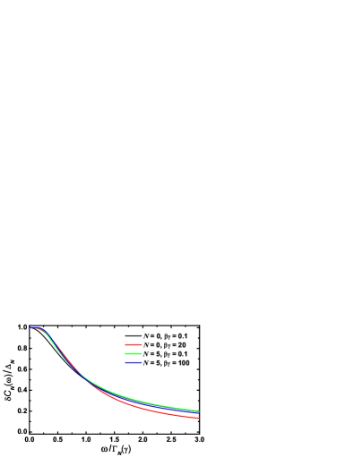
Figure 1: The deviation spectrum function $\delta C_{N}(\omega)$ of Drude bath, plotted in terms of $\delta C_{N}(\omega)/\Delta_{N}$ versus $\omega/\Gamma_{N}(\gamma)$ for some selected values of $\{N,\beta\gamma\}$, where $\Delta_{N}$ is given via Eq. (8) and $\Gamma_{N}(\gamma)$ is by the approximant of Eq. (12).

Figure 1 depicts the residue spectrum $\delta C_{N}(\omega)$, plotted in terms of $\delta C_{N}(\omega)/\Delta_{N}$ versus $\omega/\Gamma_{N}(\gamma)$ for some selected values of $\{N,\beta\gamma\}$. Used here for the $x$-axis scaling is the approximated $\Gamma_{N}(\gamma)$ value of Eq. (12). Thus this figure shows also the excellent quality of Eq. (12).

To validate the $\delta$-function approximation of $\delta C_{N}(t)$ [Eq. (8)], we examine the Kubo’s motional narrowing line shape parameter,Kub63174 ; Kub69101

$$\kappa_{N}(\gamma,\lambda)=\sqrt{\Gamma_{N}(\gamma)/\Delta_{N}}=\sqrt{r_{N}\Gamma_{N}(\gamma)/(\beta\lambda\gamma)}\,.$$ (13)

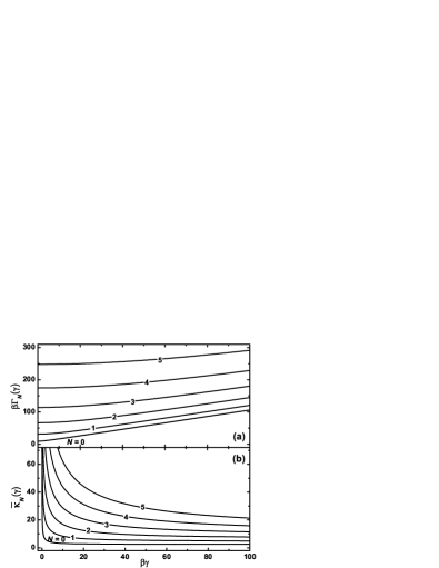
Figure 2: $\beta\Gamma_{N}(\gamma)$ and $\bar{\kappa}_{N}(\gamma)\equiv(\beta\lambda)^{1/2}\kappa_{N}(\gamma,\lambda)$ versus $\beta\gamma$.

The evaluated $\beta\Gamma_{N}(\gamma)$ and $\bar{\kappa}_{N}(\gamma)\equiv(\beta\lambda)^{1/2}\kappa_{N}(\gamma,\lambda)$, as functions of $\beta\gamma$, are depicted in Fig. 2(a) and (b), respectively.

The accuracy control criterion on the HEOM in Sec. II.1 comprises therefore the conditions under which $\delta C_{N}(t)$ and its effect on the reduced system dynamics can be treated as Markovian white noise. Apparently, it is valid when $\Gamma_{N}(\gamma)\gg\Omega_{s}$ and $\kappa_{N}(\gamma,\lambda)\gg 1$, with $\Omega_{s}$ denoting the characteristic frequency of system. We have foundXu09214111 ; Tia10114112 that the HEOM dynamics assumes numerically accurate (if not exact) when

$$\min\{\Gamma_{N}(\gamma)/\Omega_{s},\kappa_{N}(\gamma,\lambda)\}\gtrsim 5,$$ (14)

while semi-quantitative when

$$2\lesssim\min\{\Gamma_{N}(\gamma)/\Omega_{s},\kappa_{N}(\gamma,\lambda)\}\lesssim 5.$$ (15)

The above accuracy control criterions facilitate the choice of minimum $N$ for the desired quality of HEOM dynamics; see Refs. Xu09214111, and Tia10114112, for the special cases of $N=0$ and $1$, respectively.

III Numerical demonstrations

III.1 Spin-boson dynamics

To demonstrate the efficiency of HEOM and also the proposed accuracy control criterions, consider a benchmark spin-boson system, studied before by Thoss, Wang, and Miller via their numerically exact self-consistent hybrid approach.Tho012991 The system Hamiltonian is $H=\epsilon\sigma_{z}+V\sigma_{x}$, with the dissipative mode of $\hat{Q}=\sigma_{z}$, subject to Drude dissipation. Here $\sigma_{x}$ and $\sigma_{z}$ are Pauli matrices. The Rabi frequency of the system is $\Omega_{s}=2\sqrt{\epsilon^{2}+V^{2}}$. We choose the most challenging parameters used in Ref. Tho012991, , i.e., the figure 8 there, with $\epsilon/V=1$, $\lambda/V=0.25$, $\gamma/V=5$, and $\beta V=50$.

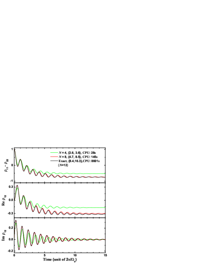
Figure 3: Evolution of the reduced spin system density matrix elements, with the same parameters as Fig. 8 of Ref. Tho012991, ; i.e., $\epsilon/V=1$, $\lambda/V=0.25$, $\gamma/V=5$, and $\beta V=50$. The accuracy control parameters are $\{\Gamma_{N}/\Omega_{s},\kappa_{N}\}=\{2.6,3.6\}$ for $N=4$ and $\{4.7,8.5\}$ for $N=8$, as indicated. The converged dynamics are identical to that of $N=10$ whose $\{\Gamma_{N}/\Omega_{s},\kappa_{N}\}=\{6.3,12.0\}$.

Figure 3 depicts the reduced system density matrix evolution, as evaluated from the HEOM at each specified environment basis set size $N$. It converges when $N\geq 10$ (by eye inspection). The accuracy control parameters $\{\Gamma_{N}/\Omega_{s},\kappa_{N}\}$ are $\{2.6,3.6\}_{N=4}$, $\{4.7,8.5\}_{N=8}$, $\{6.3,12.0\}_{N=10}$, and $\{8.4,16.3\}_{N=12}$, respectively. The CPU time listed in Fig. 3 is based on a single Intel(R) Xeon(R) processor@3.00GHz. The HEOM propagation uses the fourth-order Runge-Kutta method with time-step of $0.001/V$, together with the on-the-fly filtering algorithm Shi09084105 with error tolerance of $5\times 10^{-7}$. Evidently the numerically accurate criterion (14) and the semi-quantitative one (15) are both verified. Moreover, the $[N/N]$ PSD-based HEOM is found to be the best among all schemes we tested.

III.2 Nonlinear spectroscopy of a model exciton dimer system

We now examine the accuracy control over the $[N/N]$ PSD-based HEOM in evaluating nonlinear spectroscopic signals. We will verify again the proposed accuracy control criterions in Eqs. (14) and (15), respectively.

We first re-evaluate the figures 6 and 7 of Ref. Tia10114112, , due to a careless mistake in the excitation field configuration used there.Tia10114112note The correct signals (in rotating wave approximation) are now depicted in Figs. 4 and 5, respectively. Demonstrated are different components of the dispersed transient absorption coefficient $\alpha(\omega,t_{d})$ of a model exciton dimer system at two representing temperatures. Here, $t_{d}$ denotes the probe delay time with respect to the pump pulse. Denote also $\Delta\omega=\omega-\epsilon$, where $\epsilon=\epsilon_{1}=\epsilon_{2}$ is the on-site excitonic energy. The dimer system parametersTia10114112 are $V=-400\,{\rm cm}^{-1}$ for exciton transfer, $U=200\,{\rm cm}^{-1}$ for exciton Coulomb interaction, and $\mu_{2z}/\mu_{1z}=0.35$ for the dimer transition dipoles orientation asymmetry. The characteristic frequency of system is $\Omega_{s}=\sqrt{(\epsilon_{1}-\epsilon_{2})^{2}+4V^{2}}=2V$. The on-site Drude fluctuation parameters are $\gamma=\gamma_{1}=\gamma_{2}=600\,{\rm cm}^{-1}$ and $\lambda=\lambda_{1}=\lambda_{2}=600\,{\rm cm}^{-1}$.

The pump field is a transform-limited Gaussian pulse with 50 fs at the full width at half maximum, centered at $\omega=\epsilon$; i.e., $\Delta\omega\equiv\omega-\epsilon=0$, as indicated by the arrow in panel (a) of each Fig. 4 and Fig. 5. The peak intensity is of $\mu_{1z}E_{\rm max}=100\,$cm^-1. At $t_{d}=100$ fs the pump-transferred occupations in the single on-site exciton $|1\rangle$ and $|2\rangle$ states, and the double-exciton $|f\rangle$ state are 6.0%, 5.9%, and 1.7%, respectively, at $T=298$ K; while they are 6.3%, 6.1%, and 1.9%, respectively, at $T=77$ K. The probe field assumes in the weak and impulsive limit. Apparently, the dips appearing in the nonlinear absorptive $\alpha^{\rm NL}_{\rm A}(\omega,t_{d})$ components in the (b) panels arise mainly from the excite-state absorption to the doubly excited state. The linear emission signal [dash–curve in (a)] involves the transition from the lower lying single exciton eigenstate to ground state, without involving the the double-exciton $|f\rangle$ state. However, as the moderately strong pump field is used, the nonlinear emissive $\alpha^{\rm NL}_{\rm E}(\omega,t_{d})$ component [(c) panels] contains (in the blue side) also the contribution of the $|f\rangle$ state emission.

Figure 6 shows the two-dimensional (2D) spectroscopy $S(\omega_{3},t_{d},\omega_{1})$ of the same dimer system at $T=298$ K. As inferred from Fig. 4, the $[1/1]$ PSD-based HEOM is sufficient to give the numerically accurate results here. Both pump and probe fields are now operated in the weak and impulsive limit. As a result, $S(\omega_{3},t_{d},\omega_{1})$ resolves simply both the excitation and detection frequencies, $\omega_{1}$ and $\omega_{3}$, of the third-order optical response function, where $t_{2}$ is just the delay time $t_{d}$ of detection.Abr092350 For demonstration we examine again the absorptive (upper panels) and the emissive (middle panels) components of the experimentally measurable $S(\omega_{3},t_{d},\omega_{1})$ (bottom panels) that amounts to the $k_{I}+k_{II}$ signal.Abr092350 Evidently the dips appearing in the absorptive components are due to the excited state absorption, while the 2D emissive pathways do not include the $|f\rangle$-state emission, as the pump field is now in the weak response regime.

Figure 7 depicts the $\Delta\omega_{1}=0$ slices of the absorptive and emissive panels of Fig. 6. It thus resembles the impulsive pump counterpart of Fig. 4, except for the emissive contribution from the doubly excited state. Unlike the impulsive limit that considers only sequential processes,Muk95 the evaluation with finite pulse duration involves also coherent processes that cannot be neglected at the short time region ($t_{d}\sim 0$ here).Muk95 ; Yan906485 ; Con947855 ; Kje06024303

IV Summary

In summary, we have constructed the $[N/N]$ PSD-based HEOM, which is qualified to be the best hierarchical theory for Drude dissipation. The present work generalizes the previous $[0/0]$ and $[1/1]$ PSD-based hierarchical constructions.Xu09214111 ; Tia10114112 The proposed accuracy control criterions [Eqs. (14) and (15)] are confirmed via not only the reduced system density matrix dynamics but also nonlinear optical spectroscopy calculations. No expensive convergency check would thus be needed for the HEOM dynamics of complex open systems. HEOM for non-Drude environments that should be optimized case by case together with accuracy control criterions will be considered elsewhere.

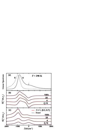
Figure 4: Dispersed transient absorption coefficient signals of the model dimer system (see text): (a) Linear absorption (A) and emission (E) signals; (b) Nonlinear absorptive $\alpha^{\rm NL}_{\rm A}(\omega,t_{d})$ component; (c) Nonlinear emissive $\alpha^{\rm NL}_{\rm E}(\omega,t_{d})$ component. The pump field is a transform-limited 50 fs-pulse of finite intensity (see text), centered at $\omega=\epsilon$; i.e., $\Delta\omega\equiv\omega-\epsilon=0$, as indicated by the arrow in panel (a). At $T=298$ K, $N=1$ is in the numerically accurate range, with $\{\Gamma_{N}/\Omega_{s},\kappa_{N}\}=\{8.3,8.7\}$ as indicated.

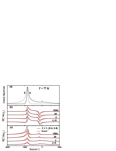
Figure 5: Same as Fig. 4, but at $T=77$ K, where $N=1$ is in the semiquantitative range, with $\{\Gamma_{N}/\Omega_{s},\kappa_{N}\}=\{2.4,2.4\}$, as indicated.

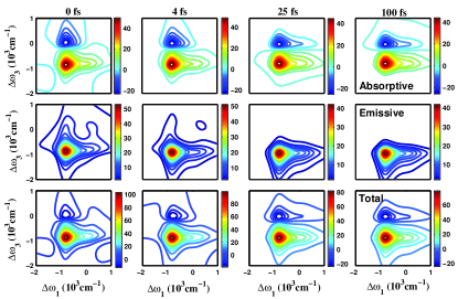
Figure 6: Two-dimensional spectroscopy $S(\omega_{3},t_{d},\omega_{1})$ of the same dimer system of Fig. 4 at $T=298$ K. Both pump and probe fields are weak and in the impulsive limit.

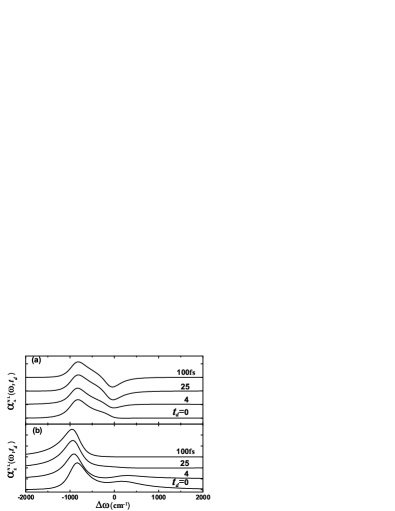
Figure 7: The $\Delta\omega_{1}=0$ slices of the absorptive and emissive panels of Fig. 6. This figure resembles the impulsive pump counterpart of Fig. 4.

- (1) A. Nitzan, Chemical Dynamics in Condensed Phases: Relaxation, Transfer and Reactions in Condensed Molecular Systems, Oxford University Press, New York, 2006.
- (2) U. Weiss, Quantum Dissipative Systems, World Scientific, Singapore, 2008, 3rd ed. Series in Modern Condensed Matter Physics, Vol. 13.
- (3) H. Kleinert, Path Integrals in Quantum Mechanics, Statistics, Polymer Physics, and Financial Markets, World Scientific, Singapore, 2009, 5th ed.
- (4) Y. J. Yan and R. X. Xu, Annu. Rev. Phys. Chem. 56, 187 (2005).
- (5) G. S. Engel et al., Nature 446, 782 (2007).
- (6) E. Collini et al., Nature 463, 644 (2010).
- (7) A. Ishizaki and G. R. Fleming, J. Chem. Phys. 130, 234110 (2009).
- (8) A. Ishizaki and G. R. Fleming, J. Chem. Phys. 130, 234111 (2009).
- (9) D. Segal and A. Nitzan, J. Chem. Phys. 117, 3915 (2002).
- (10) M. Galperin, M. A. Ratner, A. Nitzan, and A. Troisi, Science 319, 1056 (2008).
- (11) E. Pop, Nano Res 3, 147 (2010).
- (12) P. Lodahl et al., Nature 430, 654 (2004).
- (13) L. Sapienza et al., Science 327, 1352 (2010).
- (14) J. Wolters et al., Appl. Phys. Lett. 97, 141108 (2010).
- (15) Y. Tanimura, Phys. Rev. A 41, 6676 (1990).
- (16) A. Ishizaki and Y. Tanimura, J. Phys. Soc. Jpn. 74, 3131 (2005).
- (17) Y. Tanimura, J. Phys. Soc. Jpn. 75, 082001 (2006).
- (18) Y. A. Yan, F. Yang, Y. Liu, and J. S. Shao, Chem. Phys. Lett. 395, 216 (2004); J. S. Shao, J. Chem. Phys. 120, 5053 (2004).
- (19) R. X. Xu, P. Cui, X. Q. Li, Y. Mo, and Y. J. Yan, J. Chem. Phys. 122, 041103 (2005).
- (20) R. X. Xu and Y. J. Yan, Phys. Rev. E 75, 031107 (2007).
- (21) Y. Tanimura and R. Kubo, J. Phys. Soc. Jpn. 58, 101 (1989).
- (22) J. S. Jin, X. Zheng, and Y. J. Yan, J. Chem. Phys. 128, 234703 (2008).
- (23) R. P. Feynman and F. L. Vernon, Jr., Ann. Phys. 24, 118 (1963).
- (24) Q. Shi, L. P. Chen, G. J. Nan, R. X. Xu, and Y. J. Yan, J. Chem. Phys. 130, 164518 (2009).
- (25) R. X. Xu, B. L. Tian, J. Xu, Q. Shi, and Y. J. Yan, J. Chem. Phys. 131, 214111 (2009).
- (26) B. L. Tian, J. J. Ding, R. X. Xu, and Y. J. Yan, J. Chem. Phys. 133, 114112 (2010).
- (27) Erratum of Ref. Tia10114112, : The figures 6 and 7 there about the frequency-dispersed transient absorption spectrums have mistakes, and should be replaced by Figs. 4 and 5 of the present paper.
- (28) M. Tanaka and Y. Tanimura, J. Chem. Phys. 132, 214502 (2010).
- (29) A. Ishizaki and Y. Tanimura, J. Chem. Phys. 125, 084501 (2006).
- (30) A. Ishizaki and Y. Tanimura, J. Phys. Chem. A 111, 9269 (2007).
- (31) Y. Tanimura and A. Ishizaki, Acc. Chem. Res. 42, 1270 (2009).
- (32) L. P. Chen, R. H. Zheng, Q. Shi, and Y. J. Yan, J. Chem. Phys. 132, 024505 (2010).
- (33) L. P. Chen, R. H. Zheng, Y. Y. Jing, and Q. Shi, J. Chem. Phys. 134, 194508 (2011).
- (34) K. B. Zhu, R. X. Xu, H. Y. Zhang, J. Hu, and Y. J. Yan, J. Phys. Chem. B 115, 5678 (2011).
- (35) X. Zheng, J. S. Jin, and Y. J. Yan, J. Chem. Phys. 129, 184112 (2008).
- (36) X. Zheng, J. S. Jin, and Y. J. Yan, New J. Phys. 10, 093016 (2008).
- (37) X. Zheng, J. S. Jin, S. Welack, M. Luo, and Y. J. Yan, J. Chem. Phys. 130, 164708 (2009).
- (38) J. Hu, R. X. Xu, and Y. J. Yan, J. Chem. Phys. 133, 101106 (2010).
- (39) J. Hu, M. Luo, F. Jiang, R. X. Xu, and Y. J. Yan, J. Chem. Phys. 134, 244106 (2011).
- (40) M. Thoss, H. B. Wang, and W. H. Miller, J. Chem. Phys. 115, 2991 (2001).
- (41) Q. Shi, L. P. Chen, G. J. Nan, R. X. Xu, and Y. J. Yan, J. Chem. Phys. 130, 084105 (2009).
- (42) R. Kubo, J. Math. Phys. 4, 174 (1963).
- (43) R. Kubo, Adv. Chem. Phys. 15, 101 (1969).
- (44) D. Abramavicius, B. Palmieri, D. V. Voronine, F. anda, and S. Mukamel, Chem. Rev. 109, 2350 (2009).
- (45) S. Mukamel, The Principles of Nonlinear Optical Spectroscopy, Oxford University Press, New York, 1995.
- (46) Y. J. Yan and S. Mukamel, Phys. Rev. A 41, 6485 (1990).
- (47) P. Cong, Y. J. Yan, H. P. Deuel, and J. D. Simon, J. Chem. Phys. 100, 7855 (1994).
- (48) P. Kjellberg, B. Brüggemann, and T. Pullerits, Phys. Rev. B 74, 024303 (2006).