$\bf M_{h}$ in MSSM with HEAVY MAJORANA NEUTRINOS

We review the main results of the one-loop radiative corrections from the neutrino/sneutrino sector to the lightest Higgs boson mass, $M_{h}$, within the context of the so-called MSSM-seesaw scenario where right handed neutrinos and their supersymmetric partners are included in order to explain neutrino masses. For simplicity, we have restricted ourselves to the one generation case. We find sizable corrections to $M_{h}$, which are negative in the region where the Majorana scale is large ($10^{13}-10^{15}\,\,\mathrm{GeV}$) and the lightest neutrino mass is within a range inspired by data ($0.1-1$ eV). For some regions of the MSSM-seesaw parameter space, the corrections to $M_{h}$ are substantially larger than the anticipated LHC precision.

Introduction

The current experimental data on neutrino mass differences and neutrino mixing angles clearly indicate new physics beyond the so far successful Standard Model of Particle Physics (SM). In particular, neutrino oscillations imply that at least two generations of neutrinos must be massive. Therefore, one needs to extend the SM to incorporate neutrino mass terms.

We have explored the simplest version of a SUSY extension of the SM, the well known Minimal Supersymmetric Standard Model (MSSM), extended by right-handed Majorana neutrinos and where the seesaw mechanism of type I $\!{}^{{\bf?}}$ is implemented to generate the small neutrino masses. We focus here in the one generation case. The main advantage of working in a SUSY extension of the SM-seesaw is to avoid the huge hierarchy problem induced by the heavy Majorana scale.

On the other hand, it is well known that heavy Majorana neutrinos, with $m_{M}\sim 10^{13}-10^{15}$ GeV, induce large LFV rates $\!{}^{{\bf?}}$, due to their potentially large Yukawas to the Higgs sector. For the same reason, radiative corrections to Higgs boson masses due to such heavy Majorana neutrinos could also be relevant. Consequently, our study has been focused on the radiative corrections to the lightest MSSM ${\cal CP}$-even $h$ boson mass, $M_{h}$, due to the one-loop contributions from the neutrino/sneutrino sector within the MSSM-seesaw framework.

In the following we briefly review the main relevant aspects of the calculation of the mass corrections and the numerical results. For further details we address the reader to the full version of our work $\!{}^{{\bf?}}$, where also an extensive list with references to previous works can be found.

Calculation

The neutrino/sneutrino sector

The MSSM-seesaw model with one neutrino/sneutrino generation is described in terms of the well known MSSM superpotential plus the new relevant terms contained in:

$$W\,=\,\epsilon_{ij}\left[Y_{\nu}\hat{H}_{2}^{i}\,\hat{L}^{j}\hat{N}\,-\,Y_{l}\hat{H}_{1}^{i}\,\hat{L}^{j}\,\hat{R}\right]\,+\,\frac{1}{2}\,\hat{N}\,m_{M}\,\hat{N}\,,$$ (1)

where $m_{M}$ is the Majorana mass and $\hat{N}=(\tilde{\nu}_{R}^{*},(\nu_{R})^{c})$ is the additional superfield that contains the right-handed neutrino $\nu_{R}$ and its scalar partner $\tilde{\nu}_{R}$.

There are also new relevant terms in the soft SUSY breaking potential:

$$V^{\tilde{\nu}}_{\rm soft}=m^{2}_{\tilde{L}}\tilde{\nu}_{L}^{*}\tilde{\nu}_{L}+m^{2}_{\tilde{R}}\tilde{\nu}_{R}^{*}\tilde{\nu}_{R}+(Y_{\nu}A_{\nu}H^{2}_{2}\tilde{\nu}_{L}\tilde{\nu}_{R}^{*}+m_{M}B_{\nu}\tilde{\nu}_{R}\tilde{\nu}_{R}+{\rm h.c.})~{}.$$ (2)

After electro-weak (EW) symmetry breaking, the charged lepton and Dirac neutrino masses can be written as

$$m_{l}\,=\,Y_{l}\,\,v_{1}\,,\quad\quad m_{D}\,=\,Y_{\nu}\,v_{2}\,,$$ (3)

where $v_{i}$ are the vacuum expectation values (VEVs) of the neutral Higgs scalars, with $v_{1(2)}=\,v\,\cos(\sin)\beta$ and $v=174\,\,\mathrm{GeV}$.

The $2\times 2$ neutrino mass matrix is given in terms of $m_{D}$ and $m_{M}$ by:

$$M^{\nu}\,=\,\left(\begin{array}[]{cc}0&m_{D}\\ m_{D}&m_{M}\end{array}\right)\,.$$ (4)

Diagonalization of $M^{\nu}$ leads to two mass eigenstates, $n_{i}\,(i=1,2)$, which are Majorana fermions with the respective mass eigenvalues given by:

$$m_{\nu,\,N}=\frac{1}{2}\left(m_{M}\mp\sqrt{m_{M}^{2}+4m_{D}^{2}}\right)~{}.$$ (5)

In the seesaw limit, i.e. when $\xi\equiv\frac{m_{D}}{m_{M}}\ll 1~{}$

$$m_{\nu}=-m_{D}\xi+\mathcal{O}(m_{D}\xi^{3})\simeq-\frac{m_{D}^{2}}{m_{M}}~{},\quad\quad m_{N} =m_{M}+\mathcal{O}(m_{D}\xi)\simeq m_{M}~{}.$$ (6)

Regarding the sneutrino sector, the sneutrino mass matrices for the ${\cal CP}$-even, ${\tilde{M}}_{+}$, and the ${\cal CP}$-odd, ${\tilde{M}}_{-}$, subsectors are given respectively by

$${\tilde{M}}_{\pm}^{2}=\left(\begin{array}[]{cc}m_{\tilde{L}}^{2}+m_{D}^{2}+\frac{1}{2}M_{Z}^{2}\cos 2\beta&m_{D}(A_{\nu}-\mu\cot\beta\pm m_{M})\\ m_{D}(A_{\nu}-\mu\cot\beta\pm m_{M})&m_{\tilde{R}}^{2}+m_{D}^{2}+m_{M}^{2}\pm 2B_{\nu}m_{M}\end{array}\right)~{}.$$ (7)

The diagonalization of these two matrices, ${\tilde{M}}_{\pm}^{2}$, leads to four sneutrino mass eigenstates, ${\tilde{n}}_{i}\,(i=1,2,3,4)$. In the seesaw limit, where $m_{M}$ is much bigger than all the other scales the corresponding sneutrino masses are given by:

$$m_{{\tilde{\nu}_{+}},{\tilde{\nu}_{-}}}^{2} = m_{\tilde{L}}^{2}+\frac{1}{2}M_{Z}^{2}\cos 2\beta\mp 2m_{D}(A_{\nu}-\mu\cot\beta-B_{\nu})\xi~{},$$

$$m_{{\tilde{N}_{+}},{\tilde{N}_{-}}}^{2} = m_{M}^{2}\pm 2B_{\nu}m_{M}+m_{\tilde{R}}^{2}+2m_{D}^{2}~{}.$$ (8)

In the Feynman diagrammatic (FD) approach the higher-order corrected ${\cal CP}$-even Higgs boson masses in the MSSM, denoted here as $M_{h}$ and $M_{H}$, are derived by finding the poles of the $(h,H)$-propagator matrix, which is equivalent to solving the following equation $\!{}^{{\bf?}}$:

$$\left[p^{2}-m_{h}^{2}+\hat{\Sigma}_{hh}(p^{2})\right]\left[p^{2}-m_{H}^{2}+\hat{\Sigma}_{HH}(p^{2})\right]-\left[\hat{\Sigma}_{hH}(p^{2})\right]^{2}=0\,.$$ (9)

where $m_{h,H}$ are the tree level masses. The one loop renormalized self-energies, $\hat{\Sigma}_{\phi\phi}(p^{2})$, in (9) can be expressed in terms of the bare self-energies, $\Sigma_{\phi\phi}(p^{2})$, the field renormalization constants $\delta Z_{\phi\phi}$ and the mass counter terms $\delta m_{\phi}^{2}$, where $\phi$ stands for $h,H$. For example, the lightest Higgs boson renormalized self energy reads:

$$\hat{\Sigma}_{hh}(p^{2})=\Sigma_{hh}(p^{2})+\delta Z_{hh}(p^{2}-m_{h}^{2})-\delta m_{h}^{2},$$ (10)

Renormalization prescription

We have used an on-shell renormalization scheme for $M_{Z},M_{W}$ and $M_{A}$ mass counterterms and $T_{h},T_{H}$ tadpole counterterms. On the other hand, we have used a modified $\overline{\mathrm{DR}}$ scheme $\left(\mathrm{m}\overline{\mathrm{DR}}\right)$ for the renormalization of the wave function and $\tan\beta\,$. The m$\overline{\mathrm{DR}}$ scheme is very similar to the well known $\overline{\mathrm{DR}}$ scheme but instead of subtracting the usual $\Delta=\frac{2}{\epsilon}-\gamma_{E}+\log(4\pi)$ one subtracts $\Delta_{m}=\Delta-\log(m^{2}_{M}/\mu^{2}_{\overline{\mathrm{DR}}})$, hence, avoiding large logarithms of the large scale $m_{M}$. As studied in other works $\!{}^{{\bf?}}$, this scheme minimizes higher order corrections when two very different scales are involved in a calculation of radiative corrections.

Analytical and Numerical Results

In order to understand in simple terms the analytical behavior of our full numerical results we have expanded the renormalized self-energies in powers of the seesaw parameter $\xi=m_{D}/m_{M}$:

$$\hat{\Sigma}(p^{2})=\left(\hat{\Sigma}(p^{2})\right)_{m_{D}^{0}}+\left(\hat{\Sigma}(p^{2})\right)_{m_{D}^{2}}+\left(\hat{\Sigma}(p^{2})\right)_{m_{D}^{4}}+\ldots~{}.$$ (11)

The zeroth order of this expansion corresponds to the gauge contribution and it does not depend on $m_{D}$ or $m_{M}$. The rest of the terms of the expansion corresponds to the Yukawa contribution. The leading term of this Yukawa contribution is the ${\cal O}(m_{D}^{2})$ term, because it is the only one not suppressed by the Majorana scale. In fact it goes as $Y_{\nu}^{2}M^{2}_{\rm EW}$, where $M^{2}_{\rm EW}$ denotes generically the electroweak scales involved, concretely, $p^{2}$, $M_{Z}^{2}$ and $M_{A}^{2}$. In particular, the ${\cal O}(p^{2}m_{D}^{2})$ terms of the renormalized self-energy, which turn out to be among the most relevant leading contributions, separated into the neutrino and sneutrino contributions, are the following:

$$\left.\hat{\Sigma}_{hh}^{\mathrm{m}\overline{\mathrm{DR}}}\right|_{m_{D}^{2}p^{2}}\sim\left.\begin{array}[]{c}\begin{picture}(80.0,50.0) \put(0.0,0.0){} \raise 25.0pt\hbox to0.0pt{\kern 8.0pt\makebox(0.0,0.0)[r]{$h$}\hss} \ignorespaces \put(0.0,0.0){} \raise 25.0pt\hbox to0.0pt{\kern 72.0pt\makebox(0.0,0.0)[l]{$h$}\hss} \ignorespaces \put(0.0,0.0){} \raise 46.0pt\hbox to0.0pt{\kern 40.0pt\makebox(0.0,0.0)[b]{$\nu_{L}$}\hss} \ignorespaces \put(0.0,0.0){} \raise 4.0pt\hbox to0.0pt{\kern 40.0pt\makebox(0.0,0.0)[t]{$\nu_{R}$}\hss} \ignorespaces \end{picture}\end{array}+\begin{array}[]{c}\begin{picture}(80.0,50.0) \put(0.0,0.0){} \raise 25.0pt\hbox to0.0pt{\kern 8.0pt\makebox(0.0,0.0)[r]{$h$}\hss} \ignorespaces \put(0.0,0.0){} \raise 25.0pt\hbox to0.0pt{\kern 72.0pt\makebox(0.0,0.0)[l]{$h$}\hss} \ignorespaces \put(0.0,0.0){} \raise 46.0pt\hbox to0.0pt{\kern 40.0pt\makebox(0.0,0.0)[b]{$\tilde{\nu}_{L}$}\hss} \ignorespaces \put(0.0,0.0){} \raise 4.0pt\hbox to0.0pt{\kern 40.0pt\makebox(0.0,0.0)[t]{$\tilde{\nu}_{R}$}\hss} \ignorespaces \end{picture}\end{array}\right|_{m_{D}^{2}p^{2}}\sim\hskip 8.5359pt\frac{g^{2}p^{2}m_{D}^{2}c^{2}_{\alpha}}{64\pi^{2}M_{W}^{2}s^{2}_{\beta}}+\frac{g^{2}p^{2}m_{D}^{2}c^{2}_{\alpha}}{64\pi^{2}M_{W}^{2}s^{2}_{\beta}}\vspace{0.3cm}$$ (12)

Notice that the above neutrino contributions come from the Yukawa interaction $g_{h\nu_{L}\nu_{R}}=-\frac{igm_{D}\cos\alpha}{2M_{W}\sin\beta}$, which is extremely suppressed in the Dirac case but can be large in the present Majorana case. On the other hand, the above sneutrino contributions come from the new couplings $g^{\prime}_{h\tilde{\nu}_{L}\tilde{\nu}_{R}}=-\frac{igm_{D}m_{M}\cos\alpha}{2M_{W}\sin\beta}$, which are not present in the Dirac case. It is also interesting to remark that these terms, being $\sim p^{2}$ are absent in both the effective potential and the RGE approaches.

With respect to the numerical results, figure 1 exemplifies the main features of the extra Higgs mass corrections $\Delta m_{h}^{\mathrm{m}\overline{\mathrm{DR}}}$ due to neutrinos and sneutrino loops in terms of the two physical Majorana neutrino masses, $m_{N}$ and $m_{\nu}$. For values of $m_{N}<3\times 10^{13}$ GeV and $|m_{\nu}|<0.1-0.3$ eV the corrections to $M_{h}$ are positive and smaller than 0.1 GeV. In this region, the gauge contribution dominates. In fact, the wider black contour line with fixed $\Delta m_{h}^{\mathrm{m}\overline{\mathrm{DR}}}=0.09$ coincides with the prediction for the case where just the gauge part in the self-energies have been included. This means that ’the distance’ of any other contour-line respect to this one represents the difference in the radiative corrections respect to the MSSM prediction.

However, for larger values of $m_{N}$ and/or $|m_{\nu}|$ the Yukawa part dominates, and the radiative corrections become negative and larger in absolute value, up to values of -5 GeV in the right upper corner of Fig 1. These corrections grow in modulus proportionally to $m_{M}$ and $m_{\nu}$, due to the fact that the seesaw mechanism impose a relation between the three masses involved, $m_{D}^{2}=|m_{\nu}|m_{N}$.

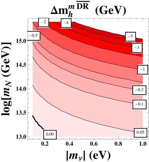
Figure 1: Contour-lines for the Higgs mass corrections from the neutrino/sneutrino sector as a function of the physical Majorana neutrino masses, light $|m_{\nu}|$ and heavy $m_{N}$. The other parameters are fixed to: $A_{\nu}=B_{\nu}=m_{\tilde{L}}=m_{\tilde{R}}=10^{3}\,\,\mathrm{GeV}$, $\tan\beta=5$, $M_{A}=200\,\,\mathrm{GeV}$ and $\mu=200\,\,\mathrm{GeV}$.

Conclusions

We have used the Feynman diagrammatic approach for the calculation of the radiative corrections to the lightest Higgs boson mass of the MSSM-seesaw. This method does not neglect the external momentum of the incoming and outgoing particles as it happens in the effective potential approach. We have performed a full calculation, obtaining not only the leading logarithmic terms as it would be the case in a RGE computation but also the finite terms, that we have seen that can be sizable for heavy Majorana neutrinos ($10^{13}-10^{15}\,\,\mathrm{GeV}$) and the lightest neutrino mass within a range inspired by data ($0.1-1$ eV). For some regions of the MSSM-seesaw parameter space, the corrections to $M_{h}$ are substantially larger ( up to -5 GeV) than the anticipated LHC precision ($\sim 200\,\,\mathrm{MeV}$) $\!{}^{{\bf?}}$.

References

References

• [1] P.ย Minkowski, Phys.ย Lett. B 67 (1977) 421;
• [2] F.ย Borzumati and A.ย Masiero, Phys.ย Rev.ย Lett. 57 (1986) 961;
M.ย Raidal et al., Eur.ย Phys.ย J.ย  C 57, 13 (2008) [arXiv:0801.1826 [hep-ph]].
• [3] S.ย Heinemeyer, M.ย J.ย Herrero, S.ย Penaranda and A.ย M.ย Rodriguez-Sanchez, JHEP 1105 (2011) 063 [arXiv:1007.5512 [hep-ph]].
• [4] M.ย Frank, T.ย Hahn, S.ย Heinemeyer, W.ย Hollik, H.ย Rzehak and G.ย Weiglein, JHEP 0702 (2007) 047 [arXiv:0611326 [hep-ph]].
• [5] J.ย Collins, F.ย Wilczek and A.ย Zee, Phys.ย Rev. D 18 (1978) 242.
• [6] G.ย Aad et al. [The ATLAS Collaboration], arXiv:0901.0512;
G.ย Bayatian et al. [CMS Collaboration], J.ย Phys. G 34 (2007) 995.