Catastrophic quenching in $\alpha\Omega$ dynamos revisited

Abstract

At large magnetic Reynolds numbers, magnetic helicity evolution plays an important role in astrophysical large-scale dynamos. The recognition of this fact led to the development of the dynamical $\alpha$ quenching formalism, which predicts catastrophically low mean fields in open systems. Here we show that in oscillatory $\alpha\Omega$ dynamos this formalism predicts an unphysical magnetic helicity transfer between scales. An alternative technique is proposed where this artifact is removed by using the evolution equation for the magnetic helicity of the total field in the shearing–advective gauge. In the traditional dynamical $\alpha$ quenching formalism, this can be described by an additional magnetic helicity flux of small-scale fields that does not appear in homogeneous $\alpha^{2}$ dynamos. In $\alpha\Omega$ dynamos, the alternative formalism is shown to lead to larger saturation fields than what has been obtained in some earlier models with the traditional formalism. We have compared the predictions of the two formalisms to results of direct numerical simulations, finding that the alternative formulation provides a better fit. This suggests that worries about catastrophic dynamo behavior in the limit of large magnetic Reynolds number are unfounded.

1. Introduction

While the possibility, and indeed need, for astrophysical dynamos was recognized quite early (Larmor, 1919), the study of dynamos has since been troubled by a number of problems. Cowling’s anti-dynamo theorem (Cowling, 1933) initially appeared to demonstrate that the entire concept was impossible, though Parker (1955) eventually discovered the physics behind what has come to be called the $\alpha$ effect. Cowling’s anti-dynamo theorem was finally shown to be largely inapplicable by analytically solvable dynamos such as the Herzenberg dynamo (Herzenberg, 1958). Once the possibility of dynamo action was demonstrated, the development of mean-field $\alpha$ dynamo theory followed (Steenbeck et al., 1966), which describes the generation of poloidal field from toroidal fields.

While the generation of toroidal magnetic fields from sheared poloidal fields is straightforward through the $\Omega$ effect, the reverse process is tricky. Without it however, dynamo action is impossible. The $\alpha$ effect, which relies on helicity (twist) in the fluid motion, allows for the generation of strong large-scale magnetic fields such as those observed in the Universe. It can drive dynamo action on its own ($\alpha^{2}$ systems), but as shear is ubiquitous in astrophysics, shear-amplified dynamo action is generally expected to outperform $\alpha^{2}$ dynamos. Accordingly, $\alpha\Omega$ dynamos, which combine the effects, are expected to be the dominant type of natural astrophysical dynamo (Hubbard & Brandenburg, 2011).

More recently however, there were indications, first suggested by Vainshtein & Cattaneo (1992), that the $\alpha$ effect decreases catastrophically already for weak mean fields in the limit of large magnetic Reynolds number (i.e. low non-dimensionalized resistivities). Such behavior would imply that mean-field dynamos driven by the $\alpha$ effect could not generate the observed large-scale magnetic fields. This claim stymied the field of large-scale dynamos for the 1990s. While strong fields are observed in nature, the theoretical understanding appeared to have been cut down. Eventually it was recognized that this behavior is not generally applicable, being restricted to two-dimensional systems, or to homogeneous (non-dynamo generated) mean fields (Blackman & Brandenburg, 2002), and large-scale dynamo simulations became common (Brandenburg, 2001; Brandenburg & Dobler, 2001). These new simulations occurred alongside the realization that magnetic helicity conservation, through the dynamical $\alpha$ quenching formalism, provides an excellent theoretical understanding of the saturation of $\alpha$–effect dynamos: the build-up of small-scale magnetic helicity quenches the $\alpha$ effect (Field & Blackman, 2002). Even so, the question of catastrophic quenching has remained open, with indications of saturated large-scale field strength decreasing with increasing magnetic Reynolds number for shearing sheets and open $\alpha^{2}$ systems (Brandenburg & Subramanian, 2005b). Further, while the saturation field strength in $\alpha^{2}$ systems with periodic or perfectly conducting boundaries has been found to be independent of the resistivity for adequately (and in practice modestly) super-critical $\mbox{\rm Re}_{M}$, the timescale to reach saturation increases linearly with $\mbox{\rm Re}_{M}$ (Brandenburg, 2001). This has led to the study of magnetic helicity fluxes (Vishniac & Cho, 2001; Brandenburg & Sandin, 2004; Mitra et al., 2010; Candelaresi et al., 2011), where the hope is that, because the build-up of small-scale magnetic helicity quenches the $\alpha$ effect, stronger and faster growing dynamos should be possible if the helicity is, instead, exported (as it cannot be destroyed except through the action of true, i.e. microphysical, dissipation).

Probing the reality of catastrophic quenching is naturally difficult. Analytical theory is impossible, and direct numerical simulations are limited to $\mbox{\rm Re}_{M}$ that, while significantly super-critical for many systems, are nevertheless orders of magnitude below those of astrophysical systems. The dynamical $\alpha$ quenching formalism allows probing large $\mbox{\rm Re}_{M}$ in systems it can handle, but its validity there cannot, of course, be directly verified. While the evidence for and against catastrophic quenching is limited, resolving the issue is a crucial step in advancing dynamo theory.

The continued improvement in techniques to measure turbulent dynamo coefficients from simulations has enabled new approaches to evaluating different formulations of the dynamical quenching formalism. In particular, the test-field method (Schrinner et al., 2005, 2007) has been used to rule out the possibility of catastrophic quenching of the turbulent magnetic diffusivity $\eta_{\it t}$ in $\alpha^{2}$ dynamos (Brandenburg et al., 2008a). Recent advances in the theory of magnetic helicity fluxes in the presence of shear (Hubbard & Brandenburg, 2011) have led us to continue these developments in dynamical quenching by revisiting earlier results from shearing systems. Somewhat surprisingly, these developments return the 1-D $\alpha$ dependent models to the first 0-D $\alpha$ dependent models (Blackman & Brandenburg, 2002). In addition, we shall extend here earlier numerical studies of $\alpha^{2}$ dynamos in open systems.

2. Mean-field modeling

2.1. Mean-field dynamo action

We reproduce here some basic results of mean-field modeling. The dynamos we will consider are in the family of $\alpha^{2}$, $\alpha\Omega$, and $\alpha^{2}\Omega$ dynamos, i.e. dynamos where the conversion of toroidal field to poloidal field occurs through the $\alpha$ effect, while the conversion of poloidal to toroidal field occurs through the $\alpha$ effect, the $\Omega$ effect, and a combination of the two. In practice, because some conversion of poloidal field to toroidal field through the $\alpha$ effect is always present, $\alpha\Omega$ dynamos are an approximation in the limit that the $\Omega$ effect is much stronger than the $\alpha$ effect. All three dynamos, in an infinite, (shearing-) periodic system arise from the same eigenvalue problem.

Although we will focus in this work on the discussion of results from numerical simulations, these results are better understood in terms of linear theory. We assume a standard, isotropic homogeneous $\alpha$, turbulent resistivity $\eta_{\it t}$, and consider a system with shear velocity $\mbox{\boldmath$U$}{}_{S}=Sx\,\hat{\!\mbox{\boldmath$y$}{}}$. We make a standard mean-field decomposition using $xy$-planar averaging throughout, with over-barred upper-case variables denoting averaged quantities and lower-cased non-overbarred referring to fluctuating quantities, e.g.,

$$\mbox{\boldmath$B$}{}=\overline{\mbox{\boldmath$B$}}{}+\bm{b},$$ (1)

$$\overline{\mbox{\boldmath$B$}}{}\equiv\frac{1}{L_{x}L_{y}}\int_{x}\int_{y}\mbox{\boldmath$B$}{}\,{\rm d}{}x\,{\rm d}{}y.$$ (2)

An important deviation from this notation is the magnetic helicity $h\equiv\mbox{\boldmath$A$}{}\cdot\mbox{\boldmath$B$}{}$, where we use

$$\overline{h}\equiv\frac{1}{L_{x}L_{y}}\int_{x}\int_{y}\mbox{\boldmath$A$}{}\cdot\mbox{\boldmath$B$}{}\,{\rm d}{}x\,{\rm d}{}y,$$ (3)

$$\overline{h}_{m}\equiv\overline{\mbox{\boldmath$A$}}{}\cdot\overline{\mbox{\boldmath$B$}}{},$$ (4)

$$\overline{h}_{f}\equiv\overline{h}-\overline{h}_{m}=\overline{\mbox{\boldmath$a$}{}\cdot\bm{b}},$$ (5)

i.e., $\overline{h}$ is the $xy$-averaged magnetic helicity density and $\overline{h}_{m}$ is the magnetic helicity density carried by the large-scale fields. Note that while $\overline{h}_{f}$ is the magnetic helicity density carried by the small-scale fields, it is still a mean quantity. We will further define $k_{\it f}$ as the wavenumber of the energy-carrying scale of the turbulence, $k_{1}$ as the scale of the mean-fields, and $B_{\rm eq}$ as the equipartition magnetic energy while working in units for which $B_{\rm eq}=u_{\rm rms}$, the rms turbulent velocity.

With these definitions and averaging choices, as long as $\overline{\bm{U}}=0$, the mean field equations are written as

$$\overline{\mbox{\boldmath${\cal E}$}}{}=\alpha\overline{\mbox{\boldmath$B$}}{}-\eta_{t}\overline{\mbox{\boldmath$J$}}{},$$ (6)

$$\frac{\partial{\overline{\mbox{\boldmath$A$}}{}}}{\partial\hskip 0.59998pt{t}}=\overline{\mbox{\boldmath${\cal E}$}}{}-\eta\overline{\mbox{\boldmath$J$}}{},$$ (7)

$$\overline{\mbox{\boldmath$B$}}{}=\mbox{\boldmath$\nabla$}{}\times\overline{\mbox{\boldmath$A$}}{},$$ (8)

where $\overline{\mbox{\boldmath$J$}}{}=\mbox{\boldmath$\nabla$}{}\times\overline{\mbox{\boldmath$B$}}{}$ is the mean current density in units for which the vacuum permeability is unity, and $\overline{\mbox{\boldmath${\cal E}$}}{}$ is the mean electromotive force, which is here expressed in terms of isotropic $\alpha$-effect and $\eta_{t}$ is the turbulent resistivity (Brandenburg, 2001). Accordingly, the mean-field problem for a one-dimensional $\alpha^{2}\Omega$ dynamo with $k_{x}=k_{y}=0$ and $k_{z}=k_{1}$ (i.e., averaging over the $xy$-plane) reduces to the eigenvalue problem

$$\lambda\,\hat{\!\mbox{\boldmath$B$}{}}=\left(\begin{array}[]{ccc}-\eta_{\rm T}k_{1}^{2}&-{\rm i}\alpha k_{1}&0\\ {\rm i}\alpha k_{1}+S&-\eta_{\rm T}k_{1}^{2}&0\\ 0&0&-\eta_{\rm T}k_{1}^{2}\end{array}\right)\,\hat{\!\mbox{\boldmath$B$}{}},$$ (9)

where $\eta_{\rm T}=\eta+\eta_{\it t}$ is the total, microphysical and turbulent, resistivity. The growing mode has eigenvalue and eigenvector

$$\lambda=|\alpha k_{1}|\sqrt{1-{\rm i}Q}-\eta_{\rm T}k_{1}^{2},$$ (10)

$$\overline{\mbox{\boldmath$B$}}{}=B_{0}\left(\sin k_{1}z,{\rm sgn}\,{}(\alpha k_{1})(1+Q^{2})^{1/4}\sin(k_{1}z+\phi),0\right),$$ (11)

where

$$Q\equiv\frac{S}{\alpha k_{1}}$$ (12)

is a measure of the relative shear and

$$\phi=1/2\arctan Q$$ (13)

is the phase between $\overline{B}_{x}$ and $\overline{B}_{y}$. The growth rate of the $\alpha^{2}\Omega$ mode is

$$\text{Re}\,\lambda=|\alpha k_{1}|\sqrt{(1+(1+Q^{2})^{1/2})/2}-\eta_{\rm T}k_{1}^{2}.$$ (14)

From the above, we draw some significant conclusions true for both $\alpha\Omega$ and the more general $\alpha^{2}\Omega$ fields:

$$|\overline{h}_{m}|=|\overline{\mbox{\boldmath$A$}}{}\cdot\overline{\mbox{\boldmath$B$}}{}|=\left|\frac{(1+Q^{2})^{1/4}}{k_{1}}B_{0}^{2}\sin\phi\right|,$$ (15)

$$\overline{\mbox{\boldmath$B$}}{}^{2}=B_{0}^{2}\left(\sin^{2}k_{1}z+(1+Q^{2})^{1/2}\sin^{2}[k_{1}z+\phi]\right),$$ (16)

i.e., the magnetic helicity density and the current helicity density $C_{m}\equiv\overline{\mbox{\boldmath$J$}}{}\cdot\overline{\mbox{\boldmath$B$}}{}$ of the mean-field are spatially uniform, while the amplitude of the mean-field is not spatially uniform if $S\neq 0$ ($Q\neq 0$ and $\phi\neq\pi/2$).

We next make the $\alpha\Omega$ approximation, assuming that $|Q|\gg 1$. We also consider only the case of $\alpha,k_{1},S\geq 0$ to simplify notation (the other cases are analogous). This implies that

$$(1+Q^{2})^{1/4}\simeq Q^{1/2}\gg 1,$$ (17)

$$\phi=\frac{\pi}{4},$$ (18)

$$\text{Re}\,\lambda=|\alpha k_{1}|\sqrt{Q/2}-\eta_{\rm T}k_{1}^{2}.$$ (19)

At constant $\eta_{\rm T}$ and $S$ then, the system will be stationary for $\alpha=\alpha_{c}$ such that

$$\alpha_{c}=\frac{2\eta_{\rm T}^{2}k_{1}^{3}}{S},\quad Q^{1/2}=\sqrt{\frac{1}{2}}\frac{S}{\eta_{\rm T}k_{1}^{2}}.$$ (20)

Further, in such a state we have

$$\frac{\overline{h}_{m}}{\langle\overline{\mbox{\boldmath$B$}}{}^{2}\rangle}=\frac{2\eta_{\rm T}k_{1}}{S}.$$ (21)

The $\alpha$ effect from maximally helical turbulence has $\alpha\sim\eta_{\it t}k_{\it f}$, so the mean magnetic field of an $\alpha\Omega$ dynamo is expected to have very low helicity. As we will see, this is an important consideration.

2.2. Catastrophic $\alpha$–quenching

Given the level of interest, it should be noted that “catastrophic” $\alpha$–quenching has not been consistently defined. We will choose the following definitions:

• Type 1 catastrophic quenching is probably the most extreme case. Here, the saturated mean-field strength varies inversely with $\mbox{\rm Re}_{M}$ (or some non-negligible negative power or similar).

• Type 2 catastrophic quenching is well understood in an $\alpha^{2}$ dynamo in a triply-periodic setup as discussed in Section 2.3. Here, the time required for final saturation scales linearly with $\mbox{\rm Re}_{M}$ (or some non-negligible positive power thereof).

A well known example of Type 2 catastrophic quenching is seen in the simulations of Brandenburg (2001), while Type 1 catastrophic quenching has been suspected to occur in the simulations of Brandenburg & Dobler (2001); Brandenburg & Subramanian (2005b), but this will be challenged by the present work.

It should be noted that both Type 1 and 2 quenchings might be less than fully catastrophic in practice. A system which rapidly reaches an $\mbox{\rm Re}_{M}$-independent field strength and then resistively decays could be Type 1 and yet have a significant field for all relevant times. Similarly, a system could take a prohibitive resistive time to fully saturate, but already reach significant field strengths on dynamical times.

Given the name $\alpha$–quenching, it would be appropriate to define a quenching type based on the value of $\alpha$. Such a definition is quite difficult however, as in the saturated regime the dynamo-driving effect counterbalances resistive decay, so the net dynamo-driving terms, including the turbulent resistivity that must accompany an $\alpha$-effect, are expected to vary with $\eta$ (and so with $\mbox{\rm Re}_{M}^{-1}$).

2.3. Dynamical $\alpha$–quenching

Dynamical $\alpha$–quenching is a theoretical advance, first introduced by Kleeorin & Ruzmaikin (1982) and more recently seen in Blackman & Brandenburg (2002), that uses the magnetic $\alpha$-effect of Pouquet et al. (1976). Under that hypothesis, the actual $\alpha$ effect in a system can be decomposed into a component due to the kinetic effect, $\alpha_{K}$, and a component due to the backreaction of the magnetic fields on the flow, $\alpha_{M}$:

$$\alpha=\alpha_{K}+\alpha_{M},\quad\alpha_{K}\simeq-\frac{\tau}{3}\overline{\mbox{\boldmath$\omega$}{}\cdot\mbox{\boldmath$u$}{}},\quad\alpha_{M}=\frac{\tau}{3\rho}\overline{\mbox{\boldmath$j$}{}\cdot\bm{b}}.$$ (22)

The mean current helicity density of the small-scale field, $\overline{\mbox{\boldmath$j$}{}\cdot\bm{b}}$, is not a tractable quantity, but in general it is well approximated by the mean magnetic helicity density of the small-scale field, $\overline{h}_{f}=\overline{\mbox{\boldmath$a$}{}\cdot\bm{b}}$, through $\overline{\mbox{\boldmath$j$}{}\cdot\bm{b}}\simeq k_{f}^{2}\overline{\mbox{\boldmath$a$}{}\cdot\bm{b}}$; see Mitra et al. (2010) for details and results in an inhomogeneous system. Recall that under this definition, small-scale magnetic helicity is a mean quantity.

The mean small-scale magnetic helicity can be found by subtracting the evolution equation of the large-scale magnetic helicity from that of the total helicity. This can be determined from the uncurled induction equation [see Section 3 of Brandenburg & Subramanian (2005a), noting the sign error for the $\mbox{\boldmath$\nabla$}{}\phi$ terms in their Equations (3.33) and (3.44)],

$$\mbox{\boldmath$E$}{}=-\mbox{\boldmath$U$}{}\times\mbox{\boldmath$B$}{}+\eta\mbox{\boldmath$J$}{},$$ (23)

$$\frac{\partial{\mbox{\boldmath$A$}{}}}{\partial\hskip 0.59998pt{t}}=-\mbox{\boldmath$E$}{}-\mbox{\boldmath$\nabla$}{}\phi,$$ (24)

$$\mbox{\boldmath$B$}{}=\mbox{\boldmath$\nabla$}{}\times\mbox{\boldmath$A$}{},$$ (25)

where $E$ is the electric field. After some vector identities, we arrive at

$$\frac{\partial{\overline{h}}}{\partial\hskip 0.59998pt{t}}=-2\eta\overline{\mbox{\boldmath$J$}{}\cdot\mbox{\boldmath$B$}{}}-\mbox{\boldmath$\nabla$}{}\cdot\overline{\mbox{\boldmath${\cal F}$}}{},$$ (26)

$$\frac{\partial{\overline{h}_{m}}}{\partial\hskip 0.59998pt{t}}=2\overline{\mbox{\boldmath${\cal E}$}}{}\cdot\overline{\mbox{\boldmath$B$}}{}-2\eta\overline{\mbox{\boldmath$J$}}{}\cdot\overline{\mbox{\boldmath$B$}}{}-\mbox{\boldmath$\nabla$}{}\cdot\overline{\mbox{\boldmath${\cal F}$}}{}_{m},$$ (27)

$$\frac{\partial{\overline{h}_{f}}}{\partial\hskip 0.59998pt{t}}=-2\overline{\mbox{\boldmath${\cal E}$}}{}\cdot\overline{\mbox{\boldmath$B$}}{}-2\eta\overline{\mbox{\boldmath$j$}{}\cdot\bm{b}}-\mbox{\boldmath$\nabla$}{}\cdot\overline{\mbox{\boldmath${\cal F}$}}{}_{f},$$ (28)

where $\overline{\mbox{\boldmath${\cal F}$}}{}=\overline{\mbox{\boldmath${\cal F}$}}{}_{m}+\overline{\mbox{\boldmath${\cal F}$}}{}_{f}$ is the sum of large-scale and small-scale magnetic helicity fluxes and $\overline{\mbox{\boldmath${\cal E}$}}{}\equiv\overline{\mbox{\boldmath$u$}{}\times\bm{b}}$; see Eq. (6). Note that the contribution of $(\mbox{\boldmath$U$}{}\times\mbox{\boldmath$B$}{})\cdot\mbox{\boldmath$B$}{}=0$ in Equation (26) is split into finite terms of opposite sign $\pm\overline{\mbox{\boldmath${\cal E}$}}{}\cdot\overline{\mbox{\boldmath$B$}}{}$ in Equations (27) and (28). The gauge term in Equation (24) is included in the flux terms; for a complete discussion see Hubbard & Brandenburg (2011). Using $\overline{\mbox{\boldmath$j$}{}\cdot\bm{b}}\simeq k_{f}^{2}\overline{\mbox{\boldmath$a$}{}\cdot\bm{b}}$, Equation (28) can be evolved in a mean-field simulation if a form for the flux term is assumed. We call this traditional dynamical $\alpha$–quenching. In homogeneous, periodic systems, such as homogeneous $\alpha^{2}$ dynamos in triply periodic cubes, the flux term vanishes, and the concept behind dynamical $\alpha$–quenching can be tested. The application of dynamical $\alpha$–quenching to this system predicts Type 2 quenching: there is an exponential growth phase which ends when $\overline{B}^{2}/B_{\rm eq}^{2}=k_{1}/k_{\it f}$ (Blackman & Brandenburg, 2002). Subsequently, there is a resistively controlled saturation phase with time $1/2\eta k_{1}^{2}$, finally ending at a saturated field strength of $\overline{B}^{2}/B_{\rm eq}^{2}=k_{\it f}/k_{1}$ (Brandenburg, 2001).

Recent work suggests that the appropriate ansatz for the flux of mean small-scale magnetic helicity is diffusive, with sub-turbulent diffusion coefficients (Hubbard & Brandenburg, 2010). However, recent work (Hubbard & Brandenburg, 2011) has also demonstrated that shear poses a unique problem which can be seen in the case of a shearing-periodic setup at a moment when all quantities are periodic except for the imposed shear flow $\mbox{\boldmath$U$}{}_{S}=Sx\ \,\hat{\!\mbox{\boldmath$y$}{}}$. In that case, the helicity flux has a horizontal component, $(\mbox{\boldmath$U$}{}_{S}\times\mbox{\boldmath$B$}{})\times\mbox{\boldmath$A$}{}$, which is not periodic and has a finite divergence. While the existence of this net flux through the shearing-periodic boundaries might be unexpected, the need for it can be simply explained. The solution of an $\alpha^{2}\Omega$ dynamo has spatially uniform large-scale helicity, as quantified by Equation (15), but the $\overline{\mbox{\boldmath${\cal E}$}}{}\cdot\overline{\mbox{\boldmath$B$}}{}$ term in Equation (27) depends on $z$. A flux term with a finite divergence is required to balance the equation. This flux term follows naturally from the requirement that whatever terms the mean electromotive force produces in the evolution equation for the magnetic helicity of the mean field, it should not affect the evolution of magnetic helicity of the total field. In other words, no terms involving $\overline{\mbox{\boldmath${\cal E}$}}{}$ should appear in the evolution equation for $\overline{\mbox{\boldmath$A$}}{}\cdot\overline{\mbox{\boldmath$B$}}{}+\overline{\mbox{\boldmath$a$}{}\cdot\bm{b}}$. Any term with $\overline{\mbox{\boldmath${\cal E}$}}{}$ in the equation for $\overline{h}_{m}$ should thus be absorbed by such a term with opposite sign in the equation for $\overline{h}_{f}$.

To elucidate this further, let us consider the equation for $\partial_{t}\overline{\mbox{\boldmath$A$}}{}=\overline{\mbox{\boldmath${\cal E}$}}{}$ for the mean field. Dotting this with $\overline{\mbox{\boldmath$B$}}{}$ gives the contribution $\overline{\mbox{\boldmath${\cal E}$}}{}\cdot\overline{\mbox{\boldmath$B$}}{}$ for the production of $\overline{\mbox{\boldmath$A$}}{}\cdot\overline{\mbox{\boldmath$B$}}{}$. We still need the contribution from $\overline{\mbox{\boldmath$A$}}{}\cdot\partial_{t}\overline{\mbox{\boldmath$B$}}{}$, i.e., $\overline{\mbox{\boldmath$A$}}{}\cdot\mbox{\boldmath$\nabla$}{}\times\overline{\mbox{\boldmath${\cal E}$}}{}$. Using the identity

$$\overline{\mbox{\boldmath$A$}}{}\cdot\mbox{\boldmath$\nabla$}{}\times\overline{\mbox{\boldmath${\cal E}$}}{}=\overline{\mbox{\boldmath${\cal E}$}}{}\cdot\mbox{\boldmath$\nabla$}{}\times\overline{\mbox{\boldmath$A$}}{}+\mbox{\boldmath$\nabla$}{}\cdot(\overline{\mbox{\boldmath${\cal E}$}}{}\times\overline{\mbox{\boldmath$A$}}{}),$$ (29)

we have

$$\frac{\partial}{\partial t}\overline{\mbox{\boldmath$A$}}{}\cdot\overline{\mbox{\boldmath$B$}}{}=2\overline{\mbox{\boldmath${\cal E}$}}{}\cdot\overline{\mbox{\boldmath$B$}}{}+\mbox{\boldmath$\nabla$}{}\cdot(\overline{\mbox{\boldmath${\cal E}$}}{}\times\overline{\mbox{\boldmath$A$}}{})+...$$ (30)

where dots indicate the presence of other terms not involving $\overline{\mbox{\boldmath${\cal E}$}}{}$ for the full equation. Thus, the evolution equation for $\overline{\mbox{\boldmath$a$}{}\cdot\bm{b}}$ must then be of the form

$$\frac{\partial}{\partial t}\overline{\mbox{\boldmath$a$}{}\cdot\bm{b}}=-2\overline{\mbox{\boldmath${\cal E}$}}{}\cdot\overline{\mbox{\boldmath$B$}}{}-\mbox{\boldmath$\nabla$}{}\cdot(\overline{\mbox{\boldmath${\cal E}$}}{}\times\overline{\mbox{\boldmath$A$}}{})+...$$ (31)

so that the evolution of $\overline{\mbox{\boldmath$A$}}{}\cdot\overline{\mbox{\boldmath$B$}}{}+\overline{\mbox{\boldmath$a$}{}\cdot\bm{b}}$ is not effected by the $\overline{\mbox{\boldmath${\cal E}$}}{}$ terms. In the traditional dynamical $\alpha$–quenching formalism, this was only true of the $2\overline{\mbox{\boldmath${\cal E}$}}{}\cdot\overline{\mbox{\boldmath$B$}}{}$ term, but the divergence of $\overline{\mbox{\boldmath${\cal E}$}}{}\times\overline{\mbox{\boldmath$A$}}{}$ had been ignored.

Allowing now for all the other terms in Equations (27) and (28), our full set of equations is

$$\frac{\partial{\overline{h}_{m}}}{\partial\hskip 0.59998pt{t}}=2\overline{\mbox{\boldmath${\cal E}$}}{}\cdot\overline{\mbox{\boldmath$B$}}{}-2\eta\overline{\mbox{\boldmath$J$}}{}\cdot\overline{\mbox{\boldmath$B$}}{}-\mbox{\boldmath$\nabla$}{}\cdot(\overline{\mbox{\boldmath${\cal F}$}}{}_{m}^{{}^{\prime}}-\overline{\mbox{\boldmath${\cal E}$}}{}\times\overline{\mbox{\boldmath$A$}}{}),$$ (32)

$$\frac{\partial{\overline{h}_{f}}}{\partial\hskip 0.59998pt{t}}=-2\overline{\mbox{\boldmath${\cal E}$}}{}\cdot\overline{\mbox{\boldmath$B$}}{}-2\eta\overline{\mbox{\boldmath$j$}{}\cdot\bm{b}}-\mbox{\boldmath$\nabla$}{}\cdot(\overline{\mbox{\boldmath${\cal F}$}}{}-\overline{\mbox{\boldmath${\cal F}$}}{}_{m}^{{}^{\prime}}+\overline{\mbox{\boldmath${\cal E}$}}{}\times\overline{\mbox{\boldmath$A$}}{}),$$ (33)

where $\overline{\mbox{\boldmath${\cal F}$}}{}_{m}^{{}^{\prime}}$ is the resistive component of $\overline{\mbox{\boldmath${\cal F}$}}{}_{m}$. When $\overline{\mbox{\boldmath$B$}}{}$ takes the form in (11) and $\overline{\mbox{\boldmath${\cal E}$}}{}=\alpha\overline{\mbox{\boldmath$B$}}{}-\eta_{\it t}\overline{\mbox{\boldmath$J$}}{}$, the $\mbox{\boldmath$\nabla$}{}\cdot(\overline{\mbox{\boldmath${\cal E}$}}{}\times\overline{\mbox{\boldmath$A$}}{})$ terms cancel the $\overline{\mbox{\boldmath${\cal E}$}}{}\cdot\overline{\mbox{\boldmath$B$}}{}$ terms. Berger & Ruzmaikin (2000) have estimated that this $\overline{\mbox{\boldmath${\cal E}$}}{}\times\overline{\mbox{\boldmath$A$}}{}$ flux can be important in the Sun.

If the flux term is not correctly handled, we can expect the generation of artificial helicity “hot-spots” through the $\overline{\mbox{\boldmath${\cal E}$}}{}\cdot\overline{\mbox{\boldmath$B$}}{}$ terms, which will nonlinearly back-react on the dynamo through Equation (22). While an adequate diffusive flux may be able to smooth out such, this poses a clear potential difficulty in applying dynamical $\alpha$–quenching to shearing systems.

If a mean-field model is solved in terms of the mean magnetic vector potential $\overline{\mbox{\boldmath$A$}}{}$ however, then $\overline{h}_{m}$ is known at every time step. Thus, rather than evolving Equation (28), one can evolve Equation (26) to find $\overline{h}_{f}=\overline{h}-\overline{h}_{m}$, avoiding the $\overline{\mbox{\boldmath${\cal E}$}}{}\cdot\overline{\mbox{\boldmath$B$}}{}$ terms. One known difficulty with this alternate technique is that spatially homogeneous components of $\overline{\mbox{\boldmath$A$}}{}$ may develop and cause spurious spatial variation in $\alpha_{M}$ when the latter is defined in terms of $\overline{\mbox{\boldmath$A$}}{}\cdot\overline{\mbox{\boldmath$B$}}{}$. This homogeneous component arises from numerical noise: as a constant $\overline{\mbox{\boldmath$A$}}{}$ is curl-free, physically motivated equations cannot generate or, unfortunately, erase it. Accordingly, we must artificially treat the issue by subtracting out the volume averaged $\langle\overline{\mbox{\boldmath$A$}}{}\rangle_{V}$. We refer to this technique of calculating $\overline{h}_{f}$ as alternate dynamical $\alpha$–quenching. For systems with no native spatial variations in $\alpha$, nor any instabilities in the spatial variation of $\alpha$, this procedure will in practice return one to the first attempts to apply dynamical $\alpha$–quenching using volume averages (Blackman & Brandenburg, 2002).

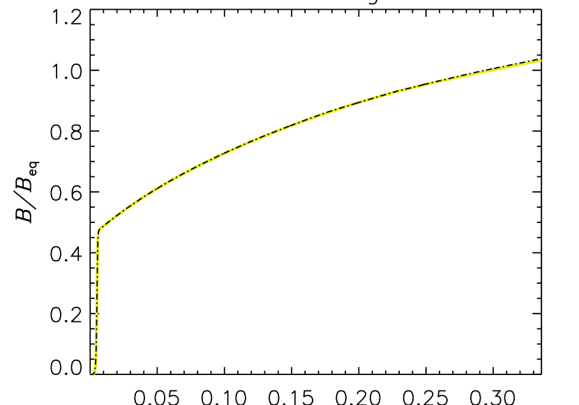
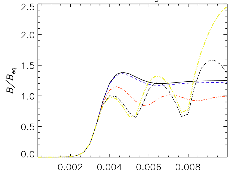
We use an $\alpha^{2}$ dynamo to test alternate dynamical $\alpha$–quenching against traditional dynamical $\alpha$–quenching (which, in this system, should be identical as there are no spatial variations and so no fluxes). We show the agreement in Figure 1. The small difference that develops is due to a smaller rms spatial noise of $\alpha_{M}$ in the alternate quenching case.

Figure 1.— Mean-field simulations for an $\alpha^{2}$ dynamo at $\mbox{\rm Re}_{M}=10^{3}$, comparing traditional (yellow/gray, solid/thick) and alternate (black/dashed) dynamical quenching models in a system where they are formally identical.

2.4. Investigation procedure

Catastrophic $\alpha$–quenching lives in the high $\mbox{\rm Re}_{M}$ regime, beyond the reach of current direct numerical simulation or laboratory experiment. This makes confirming or disproving its existence impossible. The evidence for its existence lies largely on mean-field simulations (see, e.g., Brandenburg & Subramanian, 2005b; Guerrero et al., 2010), which confirm Type 2 quenching for homogeneous isotropic periodic $\alpha^{2}$ dynamos. Further, mean-field simulations using traditional $\alpha$–quenching have strongly suggested the existence of Type 1 quenching for shearing systems.

While we cannot simulate $\alpha^{2}\Omega$ dynamos at high $\mbox{\rm Re}_{M}$, we are in a position to run modest $\mbox{\rm Re}_{M}$ shearing simulations to compare the predictions of traditional quenching (with and without diffusive magnetic helicity fluxes) with those of alternate quenching. In the latter case, we do not include uncertain diffusive fluxes because the magnetic helicity and therefore $\alpha$-effect are not expected to exhibit spatial dependencies, which we confirm.

Our procedure then is to run a direct numerical simulation of an $\alpha^{2}\Omega$ dynamo, extract the spatial dependency of $\alpha$ and compare it with the results of mean-field theories. Once mean-field theories have been weighed against the evidence, we move to large $\mbox{\rm Re}_{M}$ and examine the evidence for or against Type 1 and 2 quenching.

3. Numerics

We perform mean-field numerical simulations for a shearing sheet, with $\mbox{\boldmath$U$}{}_{S}=Sx\hat{\mbox{\boldmath$y$}{}}$, and averaging performed over the $xy$ plane, so mean quantities are only a function of $z$, reducing the problem to a one-dimensional one. Our mean field equations are evolved using the same algorithm as the Pencil Code (see below), but due to ease of implementation at the time, and low numerical load, run using the Interactive Data Language (IDL).

We formulate the mean $\overline{\mbox{\boldmath${\cal E}$}}{}$ through the standard formula (6), where $\eta_{\it t}$ is assumed not to be quenched; see Brandenburg et al. (2008a) for a numerical justification of this. The total $\alpha$ is given by the sum of the kinetic $\alpha_{K}$, presumed constant, and the magnetic $\alpha_{M}$. Accordingly, $\partial\alpha/\partial t=\partial\alpha_{M}/\partial t$. We solve the two systems of equations

$$\frac{\partial{\alpha}}{\partial\hskip 0.59998pt{t}}=-2\eta_{\it t}k_{\it f}^{2}\left(\frac{\overline{\mbox{\boldmath${\cal E}$}}{}\cdot\overline{\mbox{\boldmath$B$}}{}}{B_{\rm eq}^{2}}+\frac{\alpha-\alpha_{K}}{\eta_{\it t}/\eta}\right)+{\cal D}{}_{\alpha}\mbox{\boldmath$\nabla$}{}^{2}\alpha,$$ (34)

$$\frac{\partial{\overline{\mbox{\boldmath$B$}}{}}}{\partial\hskip 0.59998pt{t}}=\mbox{\boldmath$\nabla$}{}\times\left(\overline{\mbox{\boldmath${\cal E}$}}{}-\eta\overline{\mbox{\boldmath$J$}}{}\right),$$ (35)

for traditional quenching, see, e.g., Equations (9.14) and (9.15) of Brandenburg & Subramanian (2005a), where the helicity fluxes have been cast in the form of diffusion terms following the results of Hubbard & Brandenburg 2010, where it was found that the flux was proportional to the gradient of the magnetic helicities. The diffusive helicity flux has diffusion coefficient ${\cal D}{}_{\alpha}$ which will be scaled to $\eta_{t}$. Alternate quenching solves instead

$$\frac{\partial{\overline{h}}}{\partial\hskip 0.59998pt{t}}=-2\eta\left(\overline{\mbox{\boldmath$J$}}{}\cdot\overline{\mbox{\boldmath$B$}}{}+\alpha_{M}B_{\rm eq}^{2}/\eta_{\it t}\right),$$ (36)

$$\alpha_{M}=\eta_{\it t}k_{\it f}^{2}(\overline{h}-\overline{\mbox{\boldmath$A$}}{}\cdot\overline{\mbox{\boldmath$B$}}{})/B_{\rm eq}^{2},$$ (37)

$$\frac{\partial{\overline{\mbox{\boldmath$A$}}{}}}{\partial\hskip 0.59998pt{t}}=\overline{\mbox{\boldmath${\cal E}$}}{}-\eta\overline{\mbox{\boldmath$J$}}{}.$$ (38)

Note that for alternate quenching we also enforce $\int_{z}\overline{\mbox{\boldmath$A$}}{}\,{\rm d}{}z=0$ at every timestep to avoid drifts in the magnetic vector potential. The essential difference between the two approaches can be traced back to mutually canceling contributions to the large-scale and small-scale magnetic helicity flux of the form $\mp\overline{\mbox{\boldmath${\cal E}$}}{}\times\overline{\mbox{\boldmath$A$}}{}$.

Our direct numerical simulations are made using the Pencil Code, a finite-difference scheme sixth order in space and third order in time. In the Pencil Code runs, we use the test-field method (TFM) to determine components of the $\alpha$ tensor as a function of position. For information on TFM, see Brandenburg et al. (2008b) and Rheinhardt & Brandenburg (2010).

4. Measured $\alpha$ profiles

4.1. Direct simulation

Figure 2.— Top left panel: $\overline{\mbox{\boldmath$B$}}{}_{y}$ in a frame comoving with the dynamo wave. Top right panel: $\alpha_{xx}$. Middle panels: butterfly diagrams of components of $\alpha(z,t)$. Bottom panels: Time-averages of the middle panels. Note differing y axis scales, which implies that the quenching of $\alpha_{yy}$ is nearly uniform. See Section 4.1.

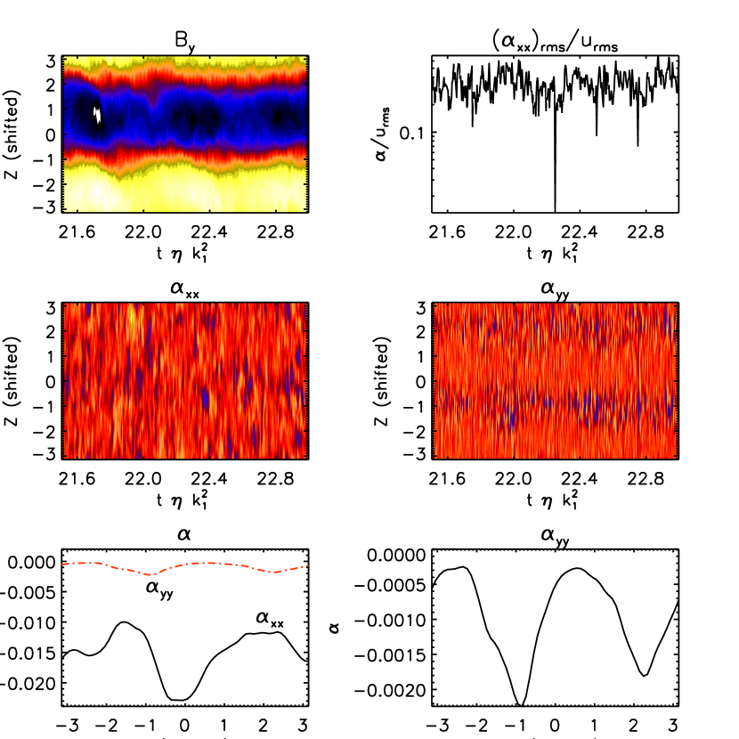
In Figure 2 we present data for the $z$ dependence of $\alpha$ well into the saturated regime for a direct simulation with $\mbox{\rm Re}_{M}=27$ and $k_{\it f}/k_{1}=3$. As in Hubbard & Brandenburg (2011), the butterfly diagrams are shifted to the frame comoving with the traveling dynamo wave, as demonstrated in the top-left panel. This allows us to take meaningful time-averages while retaining spatial information. In the top-right panel we show the volume rms of $\alpha_{xx}$ in a semi-logarithmic plot, which demonstrates that the system (including the small-scale fields in the TFM) is in a steady state for the time interval considered. The deep spike marks a reset of the test-fields (Ossendrijver et al., 2002; Hubbard et al., 2009). The middle two contour plots show the two important components of $\alpha$ in the comoving frame. The middle left panel shows $\alpha_{xx}$ which aids the $\Omega$ effect in converting the poloidal $\overline{\mbox{\boldmath$B$}}{}_{x}$ into $\overline{\mbox{\boldmath$B$}}{}_{y}$, and the middle right panel the vital $\alpha_{yy}$ which provides the conversion of the toroidal $\overline{\mbox{\boldmath$B$}}{}_{y}$ into $\overline{\mbox{\boldmath$B$}}{}_{x}$.

Figure 3.— Butterfly plots of magnetic helicity. Top panel: $\langle\mbox{\boldmath$A$}{}\rangle_{V}\cdot\overline{\mbox{\boldmath$B$}}{}$, i.e., the fictitious component of $\overline{h}_{m}$ due to a spatially homogeneous component of $A$. Middle panel: $\overline{h}_{m}$, adjusted for the top panel. Bottom panel: $\overline{h}_{f}$. While there may be some spatial structure in the bottom panels, it is intermittent in time, and the residual from a near-cancellation (the bottom two panels use a very different scale than the top one, see the color bars).

The bottom panels are time-averages of the middle panels. It appears from the contour plot that $\alpha_{yy}$ shows spatial variation, which is confirmed when a time average (in the shifted domain) is taken as seen in the bottom right panel. However, in the bottom left panel it is clear that the actual result is that $\alpha_{yy}$ is strongly quenched compared to $\alpha_{xx}$. This implies that the spatial variation seen in $\alpha_{yy}$ is merely spatial variation in the residual $\alpha$ effect: the quenching itself is nearly uniform.

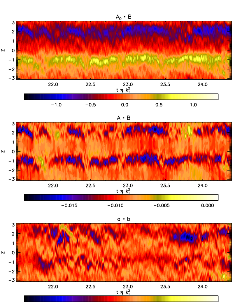
Figure 3, for the same simulation, shows the difficulty mentioned in Section 2.3, namely that a spatially homogenous component of $\langle\overline{\mbox{\boldmath$A$}}{}\rangle_{V}$ can generate a spurious magnetic helicity signal. We must also note here that the quenching is blatantly non-isotropic. A study of this effect is beyond the scope of this paper: we expect it to be a full project in its own right, and intend to study it as such.

4.2. Mean-field approaches

Figure 4.— Field and $\alpha=\alpha_{K}+\alpha_{M}$ (taken at the final time) profiles for mean-field simulations, approximately saturated. The simulations are intended to be compared with that of Figure 2, so it has the same $\mbox{\rm Re}_{M}=27$ and $k_{\it f}/k_{1}=3$. Black/solid: alternate quenching formula. Blue/dashed, red, black and yellow/dash–dotted use the conventional quenching formula with ${\cal D}{}_{\alpha}/\eta_{\it t}=10,1,0.1,0.01,0$, respectively.

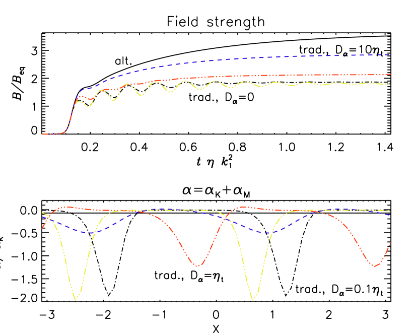
In Figure 4 we show energies and $\alpha_{M}$ profiles for mean-field simulations similar to that of Figure 2 ($\mbox{\rm Re}_{M}=27$, $k_{\it f}/k_{1}=3$). The mean-field simulations use traditional quenching with ${\cal D}{}_{\alpha}/\eta_{\it t}$ ranging from $0$ to $10$ and a run with alternate quenching. None of the traditional models match the uniform quenching that is measured in Figure 2, showing large spatial variability that derives from the $\overline{\mbox{\boldmath${\cal E}$}}{}\cdot\overline{\mbox{\boldmath$B$}}{}$ term in Equation (28), not even the model with ${\cal D}{}_{\alpha}=10\eta_{\it t}$. The decrease in spatial variation of $\alpha$ with increasing ${\cal D}{}_{\alpha}$ suggests that the traditional model could be made to function with an adequate diffusion term, but this term would need to be absurd in scale (and would hopelessly distort any simulation with “real” spatial variation in $\alpha_{M}$ that needs to be correctly captured). The alternate quenching formalism does result in the uniform quenching, which is unsurprising as it eliminates the spatial forcing from $\overline{\mbox{\boldmath${\cal E}$}}{}\cdot\overline{\mbox{\boldmath$B$}}{}$.

We take this as strong evidence that the alternate quenching formalism is superior to traditional quenching in sheared systems where drifts in $\overline{\mbox{\boldmath$A$}}{}$ are tractable – and that results obtained with traditional quenching in the presence of shear should be viewed with suspicion.

5. Mean Field: Large magnetic Reynolds numbers

5.1. Early times

Figure 5.— Field magnitudes for mean-field simulations discussed in Section 5.1, into the non-kinematic regime. The simulations use $\mbox{\rm Re}_{M}=10^{3}$, $k_{\it f}/k_{1}=3$. Black/solid: alternate quenching formula. Blue/dashed, red, black and yellow/dash–dotted use the conventional quenching formula with ${\cal D}{}_{\alpha}/\eta_{\it t}=10,1,0.1,0.01,0$, respectively. Note the oscillations, which persist at some level even with ${\cal D}{}_{\alpha}=0.1\eta_{\it t}$.

For early times, the predictions of both dynamical $\alpha$–quenching formalisms predict behavior similar to that of $\alpha^{2}$ dynamos: exponential growth of the mean fields (and corresponding growth of $\alpha_{M}$) until the total $\alpha$ effect is reduced enough that the growth rate is reduced to a fraction of its original self. This occurs when $|\alpha|=|2\eta_{\rm T}^{2}k_{1}^{3}/S|$, i.e., when

$$\left|\frac{\tau}{3}\langle\mbox{\boldmath$j$}{}\cdot\bm{b}\rangle\right|=|\alpha_{K}|-|2\eta_{\rm T}^{2}k_{1}^{3}/S|.$$ (39)

In terms of magnetic helicity, this becomes

$$|\langle\mbox{\boldmath$a$}{}\cdot\bm{b}\rangle|=k_{\it f}^{-2}\frac{3}{\tau}\left(|\alpha_{K}|-|2\eta_{\rm T}^{2}k_{1}^{3}/S|\right).$$ (40)

Using the standard approximations for fully helical turbulence (Sur et al., 2008), namely $\tau\simeq 1/u_{\text{rms}}k_{f}$, $\alpha_{K}\simeq u_{\text{rms}}/3$ and $\eta_{\it t}\simeq\tau u_{\text{rms}}^{2}/3$, and writing $B_{\rm eq}=u_{\rm rms}$, this reduces to

$$|\langle\mbox{\boldmath$a$}{}\cdot\bm{b}\rangle|\simeq\left(1-\frac{2k_{1}^{3}B_{\rm eq}}{3k_{\it f}^{2}|S|}\right)\frac{B_{\rm eq}^{2}}{k_{\it f}}.$$ (41)

As the growth is rapid, we will have $\overline{h}_{m}\simeq-\overline{h}_{f}$ during this stage, and so

$$|\overline{h}_{m}|=\left(1-\frac{2k_{1}^{3}B_{\rm eq}}{3k_{\it f}^{2}|S|}\right)\frac{B_{\rm eq}^{2}}{k_{\it f}}.$$ (42)

However, $\alpha\Omega$ dynamo mean-fields are only weakly helical, i.e. $\overline{h}_{m}\ll\overline{\mbox{\boldmath$B$}}{}^{2}/k_{1}$. Under the assumptions that the mean field is approximately stationary, and that the shear is strong enough to use Equation (21) as an approximation, Equation (42) implies that:

$$\langle\overline{\mbox{\boldmath$B$}}{}^{2}\rangle=\frac{|S|}{2\eta_{\rm T}k}\overline{h}_{m}=\left(\left|\frac{S}{2\alpha_{K}k_{1}}\right|-\frac{k_{1}^{2}}{k_{\it f}^{2}}\right)B_{\rm eq}^{2}.$$ (43)

As we have made the $\alpha\Omega$ approximation that $|S|\gg|\alpha_{K}k_{1}|$, this implies that an $\alpha\Omega$ field first feels nonlinear effects for mean-field energies that are already in super-equipartition.

In Figure 5 we show the early evolution of a mean-field dynamo with $\mbox{\rm Re}_{M}=10^{3}$, $\alpha_{K}=-1/3$, $S=1$ and $k_{\it f}/k_{1}=3$. Equation (43) implies that the exit from exponential growth occurs for $\overline{B}\approx 1.18B_{\rm eq}$, which is well captured by alternate quenching, and traditional quenching with strong diffusive fluxes.

5.2. Late times

Figure 6.— Field magnitudes, for the same mean-field simulations as Figure 5 ($\mbox{\rm Re}_{M}=10^{3}$, $k_{\it f}/k_{1}=3$), into the non-kinematic regime. Red/solid and over-plotted black/dashed: alternate quenching formula for $\mbox{\rm Re}_{M}=1000$ and $2000$ respectively. Blue/dashed, red/dash-double-dotted, black/dash-dotted and yellow/dash-double-dotted use the conventional quenching formula with ${\cal D}{}_{\alpha}/\eta_{\it t}=10,1,0.1,0$, respectively. The curve for ${\cal D}{}_{\alpha}/\eta_{\it t}=0.1$ is extremely strongly coarse-grained for visibility: the oscillations (for that run) are in fact far more frequent than shown and would be a solid band if plotted fully.

We can analytically estimate the final field strength of the dynamo for the alternate quenching formalism, while for traditional models the problem is nonlinear as can be seen in Figure 4. The final state is achieved when $\partial\overline{h}/\partial t=0$, i.e., when $\overline{\mbox{\boldmath$J$}{}\cdot\mbox{\boldmath$B$}{}}=\langle\mbox{\boldmath$j$}{}\cdot\bm{b}\rangle$. Combining this with Equation (21) and assuming that the shear is strong enough that $\alpha$ must be fully quenched, $\alpha=\alpha_{K}+\alpha_{M}\simeq 0$, we find

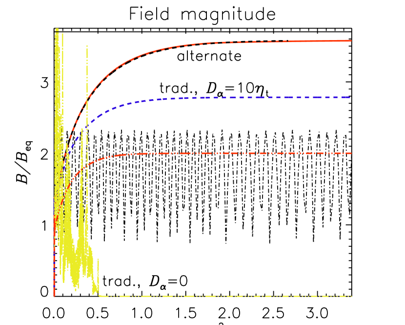
$$\overline{\mbox{\boldmath$B$}{}}^{2}\simeq|S/2\alpha_{\it K}k_{1}|\,(k_{\it f}/k_{1})^{2}B_{\rm eq}^{2}.$$ (44)

In Figure 6 we show the late time evolution of the same mean field dynamos as in Section 5.1. It is clear that, without significant (${\cal D}{}_{\alpha}>0.1\eta_{\it t}$) helicity diffusion, the solution for traditional quenching is unstable and drops to resistively small values. This is not surprising as the problem becomes highly nonlinear. However, with moderate diffusion the field strength behaves smoothly, with the final energy level increasing with diffusion coefficient. Even so, the saturation level of the traditional quenching model with ${\cal D}{}_{\alpha}=10\eta_{\it t}$ is significantly below that of the alternate quenching model. While the diffusion does smooth out the helicity hot-spots, the spatial fluctuations of $\alpha_{M}$ in Figure 4 have a noteworthy impact on the final dynamo state. Finally, the saturation level of the alternate model matches the estimate from Equation (44) of $\overline{\mbox{\boldmath$B$}{}}\simeq 3.7B_{\rm eq}$, to within the limit that an adequate residual $\alpha$ is needed to sustain the field against turbulent resistive decay. Further, the overplotted black/dashed alternate-quenching curve is for $\mbox{\rm Re}_{M}=2000$, double that of the red/solid alternate-quenching curve. The overlay implies that we have reached an asymptotic state independent of $\mbox{\rm Re}_{M}$, which is in agreement with earlier work assuming perfect spatial homogeneity (Blackman & Brandenburg, 2002) and with simulations (see Figure 6 of Käpylä & Brandenburg, 2009).

6. Direct simulations of open systems

Numerical resources limit our ability to probe the high $\mbox{\rm Re}_{M}$ regime. However, we have run three simulations of $\alpha^{2}$ dynamos in an open system, i.e., a system which can export magnetic helicity. This system is the same one as considered in Brandenburg & Subramanian (2005b): a helically forced cube, periodic in the horizontal directions and with vertical field conditions in the vertical directions, which we have run for $\mbox{\rm Re}_{M}=86$ and $156$. Additionally, as the vertical field condition is frequently used instead of a proper vacuum condition, we also performed a $\mbox{\rm Re}_{M}=156$ run with potential field condition in the vertical directions. The resulting time series are given in Figure 7. Our resolution was $128^{3}$, for runs with $u_{\text{max}}\simeq 0.15$, $u_{\rm rms}\simeq 0.05$ and $\eta=2\times 10^{-4}$ (for $\mbox{\rm Re}_{M}=86$) or $\eta=10^{-4}$ (for the other two). The velocity boundary has a stress-free vertical condition, and the entropy a symmetric one.

Figure 7.— Time series for $\alpha^{2}$ dynamos in open systems. Black/solid: potential field extrapolation in the vertical direction. Red/blue/dashed: vertical field condition on the vertical direction. Potential field and VF_b have $\mbox{\rm Re}_{M}=156$ while VF_c has $\mbox{\rm Re}_{M}=86$. The dash-double-dotted line corresponds to $1/k_{f}^{1/2}$, i.e. the energy level associated with the end of the kinematic phase.

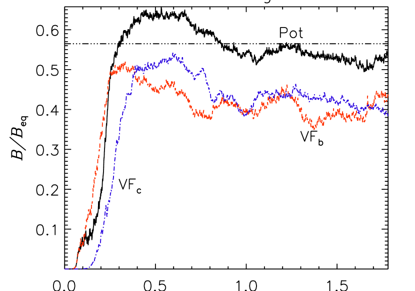
Unlike the results reported in Brandenburg & Subramanian (2005b), there is no clear indication of a reduction in the strength of the mean field for higher magnetic Reynolds number, even though the runs were followed for resistive times. However, the use of vertical field conditions as a proxy for vacuum conditions appears to be a poor one. Note that there does not appear to be a slow resistive phase. This lack is expected as the open boundaries allow the system to export total magnetic helicity (not just helicity of the small-scaled field). Thus, the system should reach a steady state where exchanges of helicity through the boundary balance preferential destruction of small-scale helicity on dynamical times, and for small total helicities.

7. Discussion and conclusions

We have used the test-field method to examine the predictions of catastrophic $\alpha$–quenching resulting from dynamically–quenched mean-field models in shearing systems. Formulations for dynamical $\alpha$–quenching which are superior for the problem of shearing systems do not predict Type 1 catastrophic quenching (reduced field strength) but do predict Type 2 quenching (long final saturation times), extending results that do not allow for spatial variations of $\alpha$ (Blackman & Brandenburg, 2002) to models that do. We have further revisited simulations of $\alpha^{2}$ dynamos in open systems and, at admittedly quite modest $\mbox{\rm Re}_{M}$, found no evidence of field strength scaling inversely with $\mbox{\rm Re}_{M}$.

The picture we see now for $\alpha$–effect dynamos, motivated by the concepts and formalism of dynamical $\alpha$–quenching, is one of exponential growth during a rapid initial saturation phase. This phase ends when the magnetic helicity in the small-scale fields is comparable to the helicity in the forcing that generates the $\alpha$–effect. At this point, the total magnetic helicity in the system has not changed from its initial value. If the system is open, exchanges with the exterior (Section 6) will tend to keep the total magnetic helicity roughly constant, and the system will then not evolve resistively. On the other hand, if the system is closed the preferential resistive destruction of magnetic helicity of the small-scale field allows a further resistive growth phase.

It is important to note that the energy in the large-scale field is bounded below by its helicity. Weakly helical large-scale fields are possible, which can have super-equipartition fields even at the end of the kinematic growth phase. Weakly helical large-scale fields are a natural product of sheared system, so rapid growth to sub-equi-, equi- and super-equipartition fields are all expected to occur in nature, although all equi- and super-equipartition fields in the high $\mbox{\rm Re}_{M}$ systems of astrophysics are expected to be weakly helical.

References

- Berger & Ruzmaikin (2000) Berger, M. A., & Ruzmaikin, A. 2000, J. Geophys. Res., 105, 10481
- Blackman & Brandenburg (2002) Blackman, E. G., & Brandenburg, A. 2002, ApJ, 579, 359
- Brandenburg (2001) Brandenburg, A. 2001, ApJ, 550, 824
- Brandenburg & Dobler (2001) Brandenburg, A., & Dobler, W. 2001, A&A, 369, 329
- Brandenburg & Sandin (2004) Brandenburg, A., & Sandin, C. 2004, A&A, 427, 13
- Brandenburg & Subramanian (2005a) Brandenburg, A., & Subramanian, K. 2005a, Phys. Rep., 417, 1
- Brandenburg & Subramanian (2005b) Brandenburg, A., & Subramanian, K. 2005b, Astron. Nachr., 326, 400
- Brandenburg et al. (2008a) Brandenburg, A., Rädler, K.-H., Rheinhardt, M., & Subramanian, K. 2008a, ApJ, 687, L49
- Brandenburg et al. (2008b) Brandenburg, A., Rädler, K.-H., & Schrinner, M. 2008b, A&A, 482, 739
- Candelaresi et al. (2011) Candelaresi, S., Hubbard, A., Brandenburg, A., & Mitra, D. 2011, Physics of Plasmas, 18, 012903
- Cowling (1933) Cowling, T. G. 1933, MNRAS, 94, 39
- Field & Blackman (2002) Field, G. B., & Blackman, E. G. 2002, ApJ, 572, 685
- Guerrero et al. (2010) Guerrero, G., Chatterjee, P., & Brandenburg, A. 2010, MNRAS, 409, 1619
- Herzenberg (1958) Herzenberg, A. 1958, Phil. Trans. R. Soc. A, 250, 543
- Hubbard & Brandenburg (2010) Hubbard, A., & Brandenburg, A. 2010, Geophys. Astrophys. Fluid Dyn., 104, 577
- Hubbard & Brandenburg (2011) Hubbard, A., & Brandenburg, A. 2011, ApJ, 727, 11
- Hubbard et al. (2009) Hubbard, A., Del Sordo, F., Käpylä, P. J., & Brandenburg, A. 2009, MNRAS, 398, 1891
- Käpylä & Brandenburg (2009) Käpylä, P. J., & Brandenburg, A. 2009, ApJ, 699, 1059
- Kleeorin & Ruzmaikin (1982) Kleeorin, N. I., & Ruzmaikin, A. A. 1982, Magnetohydrodynamics, 18, 116
- Larmor (1919) Larmor, J. 1919, Rep. Brit. Assoc. Adv. Sci., 159
- Mitra et al. (2010) Mitra, D., Candelaresi, S., Chatterjee, P., Tavakol, R., & Brandenburg, A. 2010, Astron. Nachr., 331, 130
- Ossendrijver et al. (2002) Ossendrijver, M., Stix, M., Brandenburg, A., & Rüdiger, G. 2002, A&A, 394, 735
- Parker (1955) Parker, E. N. 1955, ApJ, 122, 293
- Pouquet et al. (1976) Pouquet, A., Frisch, U., & Leorat, J. 1976, Journal of Fluid Mechanics, 77, 321
- Rheinhardt & Brandenburg (2010) Rheinhardt, M., & Brandenburg, A. 2010, å, 520, A28
- Schrinner et al. (2005) Schrinner, M., Rädler, K.-H., Schmitt, D., Rheinhardt, M., Christensen, U. 2005, Astron. Nachr., 326, 245
- Schrinner et al. (2007) Schrinner, M., Rädler, K.-H., Schmitt, D., Rheinhardt, M., Christensen, U. R. 2007, Geophys. Astrophys. Fluid Dyn., 101, 81
- Steenbeck et al. (1966) Steenbeck, M., Krause, F., Rädler, K.-H. 1966, Zeitschr. Naturforsch. A, 21, 369
- Sur et al. (2008) Sur, S., Brandenburg, A., & Subramanian, K. 2008, MNRAS, 385, L15
- Vainshtein & Cattaneo (1992) Vainshtein, S. I., & Cattaneo, F. 1992, ApJ, 393, 165
- Vishniac & Cho (2001) Vishniac, E. T., & Cho, J. 2001, ApJ, 550, 752