Unbounded Contention Resolution in
Multiple-Access Channels

Abstract

A frequent problem in settings where a unique resource must be shared among users is how to resolve the contention that arises when all of them must use it, but the resource allows only for one user each time. The application of efficient solutions for this problem spans a myriad of settings such as radio communication networks or databases. For the case where the number of users is unknown, recent work has yielded fruitful results for local area networks and radio networks, although either a (possibly loose) upper bound on the number of users needs to be known [7], or the solution is suboptimal [2], or it is only implicit [10] or embedded [6] in other problems, with bounds proved only asymptotically. In this paper, under the assumption that collision detection or information on the number of contenders is not available, we present a novel protocol for contention resolution in radio networks, and we recreate a protocol previously used for other problems [10, 6], tailoring the constants for our needs. In contrast with previous work, both protocols are proved to be optimal up to a small constant factor and with high probability for big enough number of contenders. Additionally, the protocols are evaluated and contrasted with the previous work by extensive simulations. The evaluation shows that the complexity bounds obtained by the analysis are rather tight, and that both protocols proposed have small and predictable complexity for many system sizes (unlike previous proposals).

1 Introduction

The topic of this work is the resolution of contention in settings where an unknown number of users must access a single shared resource, but multiple simultaneous accesses are not feasible. The scope of interest in this problem is wide, ranging from radio and local area networks to databases and transactional memory. (See [2] and the references therein.)

A common theme in protocols used for this problem is the adaptive adjustment of some user variable that reflects its eagerness in trying to access the shared resource. Examples of such variable are the probability of transmitting a message in a radio network or the frequency of packet transmission in a local area network. When such adjustment reduces (resp. increases) the contention, the technique is called back-off (resp. back-on). Combination of both methods are called back-on/back-off. Protocols used may be further characterized by the rate of adjustment. E.g., exponential back-off, polynomial back-on, etc. In particular, exponential back-off is widely used and it has proven to be efficient in practical applications where statistical arrival of contenders is expected. Nevertheless, worst case arrival patterns, such as bursty or batched arrivals, are frequent [17, 11].

A technique called Loglog-iterated Back-off was shown to be within a sublogarithmic factor from optimal with high probability in [2].  The protocol was presented in the context of packet contention resolution in local area networks for batched arrivals. Later on, also for batched arrivals, we presented a back-on/back-off protocol in [7], instantiated in the $k$-selection problem in Radio Networks (defined in Section 2). The latter protocol, named here Log-fails Adaptive, is asymptotically optimal for any significant probability of error, but additionally requires that some upper bound (possibly loose) on the number of contenders is known. In the present paper, we remove such requirement. In particular, we present and analyze a protocol that we call One-fail Adaptive for $k$-selection in Radio Networks. We also recreate and analyze another protocol for $k$-selection, called here Exp Back-on/Back-off, which was previously embedded in protocols for other problems and analyzed only asymptotically [10, 6]. Our analysis shows that One-fail Adaptive and Exp Back-on/Back-off, both of independent interest, resolve contention among an unknown and unbounded  number of contenders with high probability in optimal time up to constants. Additionally, by means of simulations, we evaluate and contrast the average performance of all four protocols. The simulations show that the complexity bounds obtained in the analysis (with high probability) for these protocols are rather tight for the input sizes considered. Additionally, they show that they are faster that Loglog-iterated Back-off and more predictable for all network sizes than Log-fails Adaptive.

Roadmap

The rest of the paper is organized as follows. In the following section the problem, model, related work and results are detailed. In Section 3, we introduce One-fail Adaptive and its analysis. Exp Back-on/Back-off is detailed and analyzed in Section 4. The results of the empirical contrast of all four protocols is given in Section 5 and we finish with concluding remarks and open problems in Section 6.

2 Preliminaries

A well-studied example of unique-resource contention is the problem of broadcasting information in a multiple-access channel. A multiple-access channel is a synchronous system that allows a message to be delivered to many recipients at the same time using a channel of communication but, due to the shared nature of the channel, the simultaneous introduction of messages from multiple sources produce a conflict that precludes any message from being delivered to any recipient. The particular model of multiple-access channel we consider here is the Radio Network, a model of communication network where the channel is contended (even if radio communication is not actually used [4]). We first precise our model of Radio Network as follows.

The Model:

We consider a Radio Network comprised of $n$ stations called nodes. Each node is assumed to be potentially reachable from any other node in one communication step, hence, the network is characterized as single-hop or one-hop indistinctively. Before running the protocol, nodes have no information, not even the number of nodes $n$ or their own label. Time is supposed to be slotted in communication steps. Assuming that the computation time-cost is negligible in comparison with the communication time-cost, time efficiency is studied in terms of communication steps only. The piece of information assigned to a node in order to deliver it to other nodes is called a message. The assignment of a message is due to an external agent and such an event is called a message arrival. Communication among nodes is carried out by means of radio broadcast on a shared channel. If exactly one node transmits at a communication step, such a transmission is called successful or non-colliding, we say that the message was delivered, and all other nodes receive such a message. If more than one message is transmitted at the same time, a collision occurs, the messages are garbled, and nodes only receive interference noise. If no message is transmitted in a communication step, nodes receive only background noise. In this work, nodes can not distinguish between interference noise and background noise, thus, the channel is called without collision detection. Each node is in one of two states, active if it holds a message to deliver, or idle otherwise. As in [2, 15, 10], we assume that a node becomes idle upon delivering its message, for instance when an explicit acknowledgement is received (like in the IEEE 802.11 Medium Access Control protocol [1]). For settings where the channel does not provide such functionality, such as Sensor Networks, a hierarchical infrastructure may be predefined to achieve it [6], or a leader can be elected as the node responsible for acknowledging successful transmissions [22].

One of the problems that require contention resolution in Radio Networks is the problem known in the literature as all-broadcast [4], or $k$-selection [15]. In $k$-selection, a set of $k$ out of $n$ network nodes have to access a unique shared channel of communication, each of them at least once. As in [2, 15, 10], in this paper we study $k$-selection when all messages arrive simultaneously, or in a batch. Under this assumption the $k$-selection problem is called static. A dynamic counterpart where messages arrive at different times was also studied [15].

The Problem:

Given a Radio Network where $k$ network nodes are activated by a message that arrives simultaneously to all of them, the static $k$-selection problem is solved when each node has delivered its message.

Related Work:

A number of fruitful results for contention resolution have been obtained assuming availability of collision detection. Martel presented in [18] a randomized adaptive protocol for $k$-Selection that works in $O(k+\log n)$ time in expectation. As argued by Kowalski in [15], this protocol can be improved to $O(k+\log\log n)$ in expectation using Willard’s expected $O(\log\log n)$ selection protocol of [23]. In the same paper, Willard shows that, for any given protocol, there exists a choice of $k\leq n$ such that selection takes $\Omega(\log\log n)$ expected time for the class of fair selection protocols (i.e., protocols where all nodes use the same probability of transmission to transmit in any given time slot). For the case in which $n$ is not known, in the same paper a $O(\log\log k)$ expected time selection protocol is described, again, making use of collision detection. If collision detection is not available, using the techniques of Kushilevitz and Mansour in [16], it can be shown that, for any given protocol, there exists a choice of $k\leq n$ such that $\Omega(\log n)$ is a lower bound in the expected time to get even the first message delivered.

Regarding deterministic solutions, the $k$-Selection problem was shown to be in $O(k\log(n/k))$ already in the 70’s by giving adaptive protocols that make use of collision detection [3, 12, 19]. In all these results the algorithmic technique, known as tree algorithms, relies on modeling the protocol as a complete binary tree where the messages are placed at the leaves. Later, Greenberg and Winograd [9] showed a lower bound for that class of protocols of $\Omega(k\log_{k}n)$. Regarding oblivious algorithms, Komlòs and Greenberg [14] showed the existence of $O(k\log(n/k))$ solutions even without collision detection but requiring knowledge of $k$ and $n$. More recently, Clementi, Monti, and Silvestri [5] showed a lower bound of $\Omega(k\log(n/k))$, which also holds for adaptive algorithms if collision detection is not available. In [15], Kowalski presented the construction of an oblivious deterministic protocol that, using the explicit selectors of Indyk [13], gives a $O(k\mathop{\mathrm{polylog}}n)$ upper bound without collision detection.

In [8], Gerèb-Graus and Tsantilas presented an algorithm that solves the problem of realizing arbitrary $h$-relations in an $n$-node network, with probability at least $1-1/n^{c},c>0$, in $\Theta(h+\log n\log\log n)$ steps. In an $h$-relation, each processor is the source as well as the destination of at most $h$ messages. Making $h=k$ this protocol can be used to solve static $k$-selection. However, it requires that nodes know $h$.

Extending previous work on tree algorithms, Greenberg and Leiserson [10] presented randomized routing strategies in fat-trees for bounded number of messages. Underlying their algorithm lies a sawtooth technique used to “guess” the appropriate value for some critical parameter (load factor), that can be used to “guess” the number of contenders in static $k$-selection. Furthermore, modulo choosing the appropriate constants, Exp Back-on/Back-off uses the same sawtooth technique. Their algorithm uses $n$ and it is analyzed only asymptotically.

Monotonic back-off strategies for contention resolution of batched arrivals of $k$ packets on simple multiple access channels, a problem that can be seen as static $k$-selection, have been analyzed in [2]. In that paper, it is shown that $r$-exponential back-off, a monotonic technique used widely that has proven to be efficient for many practical applications is in $\Theta(k\log^{\log r}k)$ for batched arrivals. The best strategy shown is the so-called loglog-iterated back-off with a makespan in $\Theta(k\log\log k/\log\log\log k)$ with probability at least $1-1/k^{c},c>0$, which does not use any knowledge of $k$ or $n$. In the same paper, the sawtooth technique used in [10] is informally described in a paragraph while pointing out that it yields linear time for contention resolution thanks to non-monotonicity, but no analysis is provided.

Later on, Farach-Colton and Mosteiro presented an optimal protocol for Gossiping in Radio Networks in [6]. The sawtooth technique embedded in [10] is used in that paper as a subroutine to resolve contention in linear time as in Exp Back-on/Back-off. However, the algorithm makes use of $n$ to achieve the desired probability of success and the analysis is only asymptotical.

A randomized adaptive protocol for static $k$-selection in a one-hop Radio Network without collision detection was presented in [7]. The protocol is shown to solve the problem in $(e+1+\xi)k+O(\log^{2}(1/\varepsilon))$ steps with probability at least $1-2\varepsilon$, where $\xi>0$ is an arbitrarily small constant and $0<\varepsilon\leq 1/(n+1)$. Modulo a constant factor, the protocol is optimal if $\varepsilon\in\Omega(2^{-\sqrt{n}})$. However, the algorithm makes use of the value of $\varepsilon$, which must be upper bounded as above in order to guarantee the running time. Therefore, knowledge of $n$ is required.

Our Results:

In this paper, we present a novel randomized protocol for static $k$-selection in a one-hop Radio Network, and we recreate a previously used technique suiting the constants for our purpose and without making use of $n$. Both protocols work without collision detection and do not require information about the number of contenders. As mentioned, these protocols are called One-fail Adaptive and Exp Back-on/Back-off. It is proved that One-fail Adaptive solves static $k$-selection within $2(\delta+1)k+O(\log^{2}k)$ steps, with probability at least $1-2/(1+k)$, for ${\mathrm{e}}<\delta\leq\sum_{j=1}^{5}(5/6)^{j}$. On the other hand, Exp Back-on/Back-off is shown to solve static $k$-selection within $4(1+1/\delta)k$ steps with probability at least $1-1/k^{c}$ for some constant $c>0$, $0<\delta<1/{\mathrm{e}}$, and big enough $k$. Given that $k$ is a lower bound for this problem, both protocols are optimal (modulo a small constant factor) for big enough number of contenders.

Observe that the bounds and the probabilities obtained are given as functions of the parameter $k$, as done in [2], since this is the input parameter of our version of the problem. A fair comparison with the results obtained as function of $k$ and $n$ would require that $k$ is large enough, so that $n=\Omega(k^{c})$, for some constant $c$. Both protocols presented are of interest because, although protocol Exp Back-on/Back-off is simpler, One-fail Adaptive achieves a better multiplicative factor, although the constant in the sublinear additive factor may be big for small values of $k$.

Additionally, results of the evaluation by simulation of the average behavior of One-fail Adaptive and Exp Back-on/Back-off and a comparison with Log-fails Adaptive and Loglog-iterated Back-off are presented. Both algorithms One-fail Adaptive and Exp Back-on/Back-off run faster than Loglog-iterated Back-off on average, even for small values of $k$. Although Loglog-iterated Back-off has higher asymptotic complexity, one may have expected that it may run fast for small networks. On the other hand, the knowledge on a bound of $k$ assumed by Log-fails Adaptive seems to provide an edge with respect to One-fail Adaptive and Exp Back-on/Back-off for large values of $k$. However, Log-fails Adaptive has a much worse behavior than the proposed protocols for small to moderate network sizes ($k\leq 10^{5}$). In any case, for all values of $k$ simulated, One-fail Adaptive and Exp Back-on/Back-off have a very stable and efficient behavior.

3 One-fail Adaptive

As in Log-fails Adaptive [7], One-fail Adaptive is composed by two interleaved randomized algorithms, each intended to handle the communication for different levels of contention. One of the algorithms, which we call AT, is intended for delivering messages while the number of nodes contending for the channel is above some logarithmic threshold (to be defined later). The other algorithm, called BT, has the purpose of handling message delivery after that number is below that threshold. Nonetheless, a node may transmit using the BT (resp. AT) algorithm even if the number of messages left to deliver is above (resp. below) that threshold.

Both algorithms, AT and BT, are based on transmission trials with certain probability and what distinguishes them is just the specific probability value used. It is precisely the particular values of probability used in each algorithm what differentiates One-fail Adaptive from Log-fails Adaptive. For the BT algorithm, the probability of transmission is inversely logarithmic on the number of messages already transmitted, while in Log-fails Adaptive that probability was fixed. For the AT algorithm the probability of transmission is the inverse of an estimation on the number of messages left to deliver. In One-fail Adaptive this estimation is updated continuously, whereas in Log-fails Adaptive it was updated after some steps without communication. These changes yield a protocol still linear, but now it is not necessary to know $n$. Further details can be seen in Algorithm 1.

For clarity, Algorithms AT and BT are analyzed separately taking into account in both analyses the presence of the other. We show the efficiency of the AT algorithm in producing successful transmissions while the number of messages left is above some logarithmic threshold, and the efficiency of the BT algorithm handling the communication after that threshold is crossed. For the latter, we use standard probability computations to show our time upper bound. For the AT algorithm, we use concentration bounds to show that the messages are delivered with large enough probability, while the density estimator $\widetilde{\kappa}$ does not exceed the actual number of messages left. This second proof is more involved since it requires some preliminary lemmas. We establish here the main theorem, which is direct consequence of the lemmata described that can be found in the Appendix.

Theorem 3.1

For any $e<\delta\leq\sum_{j=1}^{5}(5/6)^{j}$ and for any one-hop Radio Network under the model detailed in Section 1, One-fail Adaptive solves static $k$-selection within $2(\delta+1)k+O(\log^{2}k)$ communication steps, with probability at least $1-2/(1+k)$.

upon message arrival do $\widetilde{\kappa}\leftarrow\delta+1$ // Density estimator

$\sigma\leftarrow 0$ // Messages-received counter

start tasks $1,2$ and $3$

Task 1 foreach $\textnormal{{communication-step}}=1,2,\dots$ do if $\textnormal{{communication-step}}\equiv 0\pmod{2}$ then // BT-step transmit $\langle x,\textnormal{{message}}\rangle$ with prob $1/(1+\log(\sigma+1))$

else  // AT-step transmit $\langle x,\textnormal{{message}}\rangle$ with probability $1/\widetilde{\kappa}$

$\widetilde{\kappa}\leftarrow\widetilde{\kappa}+1$

Task 2 upon reception from other node do $\sigma\leftarrow\sigma+1$

if $\textnormal{{communication-step}}\equiv 0\pmod{2}$ then // BT-step $\widetilde{\kappa}\leftarrow\max\{\widetilde{\kappa}-\delta,\delta+1\}$

else  // AT-step $\widetilde{\kappa}\leftarrow\max\{\widetilde{\kappa}-\delta-1,\delta+1\}$

Task 3 upon message $delivery$ stop

Algorithm 1 One-fail Adaptive. Pseudocode for node $x$. $\delta$ is a constant such that $e<\delta\leq\sum_{j=1}^{5}(5/6)^{j}$.

10

10

10

10

10

10

10

10

10

10

4 Exp Back-on/Back-off

The algorithm presented in this section is based in contention windows. That is, each node repeatedly chooses uniformly one time slot within an interval, or window, of time slots to transmit its message. Regarding the size of such window, our protocol follows a back-on/back-off strategy. Namely, the window is increased in an outer loop and decreased in an inner loop, as detailed in Algorithm 2.

for $i=\{1,2,\dots\}$ do $w\leftarrow 2^{i}$

while $w\geq 1$ do Choose uniformly a step within the next $w$ steps

$w\leftarrow w\cdot(1-\delta)$

Algorithm 2 Window size adjustment in Exp Back-on/Back-off. $0<\delta<1/\mathrm{e}$ is a constant.

3

3

3

The intuition for the algorithm is as follows. Let $m$ be the number of messages left at a given time right before using a window of size $w$. We can think of the algorithm as a random process where $m$ balls (modelling the messages) are dropped uniformly in $w$ bins (modelling time slots). We will show that, if $m\leq w$, for large enough $m$, with high probability, at least a constant fraction of the balls fall alone in a bin. Now, we can repeat the process removing this constant fraction of balls and bins until all balls have fallen alone. Since nodes do not know $m$, the outer loop increasing the size of the window is necessary. The analysis follows.

Lemma 1

For $k\geq m\geq(2{\mathrm{e}}/(1-{\mathrm{e}}\delta)^{2})(1+(\beta+1/2)\ln k)$, $0<\delta<1/{\mathrm{e}}$, $m\leq w$, and $\beta>0$, if $m$ balls are dropped in $w$ bins uniformly at random, the probability that the number of bins with exactly one ball is less than $\delta m$ is at most $1/k^{\beta}$.

Proof

Since a bigger number of bins can only reduce the number of bins with more than one ball, if the claim holds for $w=m$ it also holds for $w>m$. Thus, it is enough to prove the first case. The probability for a given ball to fall alone in a given bin is $(1/m)(1-1/m)^{m-1}\geq 1/({\mathrm{e}}m)$. Let $X_{i}$ be a random variable that indicates if there is exactly one ball in bin $i$. Then, $Pr(X_{i}=1)\geq 1/{\mathrm{e}}$. To handle the dependencies that arise in balls and bins problems, we approximate the joint distribution of the number of balls in all bins by assuming the load in each bin is an independent Poisson random variable with mean 1. Let $X$ be a random variable that indicates the total number of bins with exactly one ball. Then, $\mu=E[X]=m/{\mathrm{e}}$. Using Chernoff-Hoeffding bounds [21], $Pr(X\leq\delta m)\leq\exp\left(-m\left(1-{\mathrm{e}}\delta\right)^{2}/(2{\mathrm{e}})\right)$, because $0<\delta<1/{\mathrm{e}}$.

As shown in [21], any event that takes place with probability $p$ in the Poisson case takes place with probability at most $p{\mathrm{e}}\sqrt{m}$ in the exact case. Then, we want to show that $\exp\left(-m(1-{\mathrm{e}}\delta)^{2}/(2{\mathrm{e}})\right){\mathrm{e}}\sqrt{m}\leq k^{-\beta}$, which is true for $m\geq\frac{2{\mathrm{e}}}{(1-{\mathrm{e}}\delta)^{2}}\left(1+\left(\frac{1}{2}+\beta\right)\ln k\right)$. ∎

Theorem 4.1

For any constant $0<\delta<1/{\mathrm{e}}$, Exp Back-on/Back-off solves static $k$-selection within $4(1+1/\delta)k$ steps with probability at least $1-1/k^{c}$, for some constant $c>0$ and big enough $k$.

Proof

Consider an execution of the algorithm on $k$ nodes. Let a round be the sequence of time steps corresponding to one iteration of the inner loop of Algorithm 2, i.e. the time steps of a window. Let a phase be the sequence of rounds corresponding to one iteration of the outer loop of Algorithm 2, i.e. when the window is monotonically reduced.

Consider the first round when $k\leq w<2k$. Assume no message was transmitted successfully before. (Any messages transmitted could only reduce the running time.) By Lemma 1, we know that, for $0<\delta<1/\mathrm{e}$ and $\beta>0$, at least $\delta k$ messages are transmitted in this round with probability at least $1-1/k^{\beta}$, as long as $k\geq\tau$, where $\tau\triangleq(2{\mathrm{e}}/(1-{\mathrm{e}}\delta)^{2})(1+(\beta+1/2)\ln k)$.

Conditioned on this event, for some $\delta_{1}\geq\delta$ fraction of messages transmitted in the first round, using the same lemma we know that in the following round at least $\delta(1-\delta_{1})k$ messages are transmitted with probability at least $1-1/k^{\beta}$, as long as $(1-\delta_{1})k\geq\tau$. This argument can be repeated for each subsequent round until the number of messages left to be transmitted is less than $\tau$. Furthermore, given that the size of the window is monotonically reduced within a phase until $w=1$, even if the fraction of messages transmitted in each round is just $\delta$, the overall probability of reducing the number of messages left from $k$ to $\tau$ within this phase is at least $(1-1/k^{\beta})^{\log_{1/(1-\delta)}(2k)}$.

Consider now the first round of the following phase, i.e. when $2k\leq w<4k$. Assume that at most $\tau$ nodes still hold a message to be transmitted. Using the union bound, the probability that two or more of $m$ nodes choose a given step in a window of size $w$ is at most $\binom{m}{2}/w^{2}$. Applying again the union bound, the probability that in any step two or more nodes choose to transmit is at most $\binom{m}{2}/w\leq\binom{\tau}{2}/(2k)=\tau(\tau+1)/(4k)$.

Therefore, using conditional probability, in order to complete the proof, it is enough to show that

$$\left(1-\frac{\tau(\tau+1)}{4k}\right)\left(1-\frac{1}{k^{\beta}}\right)^{\log_{1/(1-\delta)}(2k)} \geq 1-\frac{1}{k^{c}},\textrm{ for some constant $c>0$}$$

$$\exp\left(-\frac{\tau(\tau+1)}{4k-\tau(\tau+1)}-\frac{\log_{1/(1-\delta)}(2k)}{k^{\beta}-1}\right) \geq\exp\left(-\frac{1}{k^{c}}\right)$$

$$\frac{\tau(\tau+1)}{4k-\tau(\tau+1)}+\frac{\log_{1/(1-\delta)}(2k)}{k^{\beta}-1} \leq\frac{1}{k^{c}}.$$ (1)

Given that $\delta$ is a constant and fixing $\beta>0$ as a constant, Inequality 1 is true for some constant $c<\min\{1,\beta\}$, for big enough $k$. Telescoping the number of steps up to the first round when $w=4k$, the running time is less than $4k+2k\sum_{i=0}^{\infty}\sum_{j=0}^{\infty}(1-\delta)^{j}/2^{i}=4(1+1/\delta)k$. ∎

5 Evaluation

In order to evaluate the expected behavior of the algorithms One-fail Adaptive and Exp Back-on/Back-off, and compare it with the previously proposed algorithms Loglog-iterated Back-off and Log-fails Adaptive, we have simulated the four algorithms. The simulations measure the number of steps that the algorithms take until the static $k$-selection problem has been solved, i.e., each of the $k$ activated nodes of the Radio Network has delivered its message, for different values of $k$. Several of the algorithms have parameters that can be adapted. The value of these parameters is the same for all the simulations of the same algorithm (except the parameter $\varepsilon$ of Log-fails Adaptive that has to depend on $k$). For Exp Back-on/Back-off the parameter is chosen to be $\delta=0.366$. For One-fail Adaptive the parameter is chosen to be $\delta=2.72$. For Log-fails Adaptive, the parameters (see their meaning in [7]) are chosen to be $\xi_{\delta}=\xi_{\beta}=0.1$ and $\varepsilon\approx 1/(k+1)$, while two values of $\xi_{t}$ have been used, $\xi_{t}=1/2$ and $\xi_{t}=1/10$. Finally, Loglog-iterated Back-off is simulated with parameter $r=2$ (see [2]).

Figure 1 presents the average number of steps taken by the simulation of the algorithms. The plot shows the the average of 10 runs for each algorithm as a function of $k$. In this figure it can be observed that Log-fails Adaptive takes significantly larger number of steps than the other algorithms for moderately small values of $k$ (up to $10^{5}$). Beyond $k=10^{5}$ all algorithms seem to have a similar behavior.

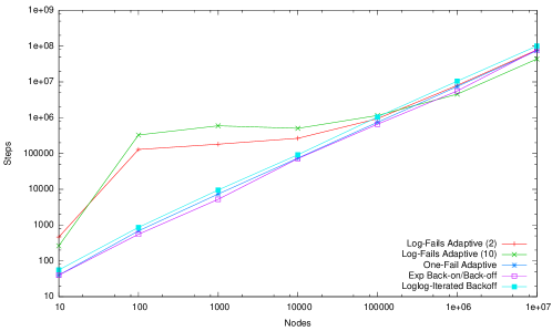
Figure 1: Number of steps to solve static $k$-selection, per number of nodes $k$.

$k$	$10$	$10^{2}$	$10^{3}$	$10^{4}$	$10^{5}$	$10^{6}$	$10^{7}$	Analysis
Log-fails Adaptive $\xi_{t}=1/2$	46.4	1292.4	181.9	26.6	9.4	8.0	7.8	7.8
Log-fails Adaptive $\xi_{t}=1/10$	26.3	3289.2	593.8	50.3	11.5	4.5	4.4	4.4
One-fail Adaptive	4.0	6.9	7.4	7.4	7.4	7.4	7.4	7.4
Exp Back-on/Back-off	4.0	5.5	5.2	7.2	6.6	5.6	7.9	14.9
Loglog-iterated Back-off	5.6	8.6	9.6	9.2	10.5	10.5	10.1	$\Theta\left(\frac{\log\log k}{\log\log\log k}\right)$

Table 1: Ratio steps/nodes as a function of the number of nodes $k$.

A higher level of detail can be obtained by observing Table 1, which presents the ratio obtained by dividing the number of steps (plotted in Figure 1) by the value of $k$, for each $k$ and each algorithm. In this table, the bad behavior of Log-fails Adaptive for moderate values of $k$ can be observed, with values of the ratio well above those for large $k$. It seems like the value of $\xi_{t}$ used has an impact in this ratio, so that the smaller value $\xi_{t}=1/10$ causes larger ratio values. Surprisingly, for large values of $k$ ($k\geq 10^{6}$), the ratios observed are almost exactly the constant factors of $k$ obtained from the analysis [7]. (Recall that all the analyses we refer to are with high probability while the simulation results are averages.) This may indicate that the analysis with high probability is very tight and that the term $O(\log^{2}(1/\varepsilon))$ that appears in the complexity expression is mainly relevant for moderate values of $k$. The ratio obtained for large $k$ by Log-fails Adaptive with $\xi_{t}=1/10$ is the smallest we have obtained in the set of simulations. Loglog-iterated Back-off, on its hand, seems to have a constant ratio of around $10$. In reality this ratio is not constant but, since it is sublogarithmic, this fact can not be observed for the (relatively small) values of $k$ simulated.

Regarding the ratios obtained for the algorithms proposed in this paper, they seem to show that the constants obtained in the analyses (with high probability) are very accurate. Starting at moderately large values of $k$ ($10^{3}$ and up) the ratio for One-fail Adaptive becomes very stable and equal to the value of $7.4$ obtained in the analysis. The ratios for the Exp Back-on/Back-off simulations, on their hand, move between 4 and 8, while the analysis for the value of $\delta$ used yields a constant factor of 14.9. Hence, the ratios are off by only a small constant factor. To appreciate these values it is worth to note that the smallest ratio expected by any algorithm in which nodes use the same probability at any step is $e$, so these values are only a small factor away from this optimum ratio. In summary, the algorithms proposed here have small and stable ratios for all values of $k$ considered.

6 Conclusions and Open Problems

In this work, we have shown optimal randomized protocols (up to constants) for static $k$-selection in Radio Networks that do not require any knowledge on the number of contenders. Future work includes the study of the dynamic version of the problem when messages arrive at different times under the same model, either assuming statistical or adversarial arrivals. The stability of monotonic strategies (exponential back-off) has been studied in [2]. In light of the improvements obtained for batched arrivals, the application of non-monotonic strategies to the dynamic problem is promising.

Appendix

Appendix 0.A Lemmata of the analysis of One-fail Adaptive

For clarity, Algorithms AT and BT are analyzed separately taking into account in both the presence of the other. Communication steps are referred to by the name of the algorithm used, i.e. a communication step is either an AT-step or a BT-step. The following notation will be used throughout the analysis.

Let $\kappa$ be the number of messages not delivered yet (i.e., the number of active nodes), called the density, and let $\widetilde{\kappa}$ be called the density estimator. Consider the execution of Algorithm 1 divided in rounds as follows. The first round begins with the first step of the execution, and a new round starts on each step that $\widetilde{\kappa}$ reaches or exceeds a multiple of $\tau\triangleq 300\delta\ln(1+k)$ for the first time. (Hence, a new round may start only in an AT-step.) More precisely, let the rounds be numbered as $r\in\{1,2,\dots\}$ and the AT-steps within a round as $t\in\{1,2,\dots\}$. Let $T_{r}$ be the set of AT-steps of round $r$. Let $\widetilde{\kappa}_{r,t}$ be the density estimator used at the AT-step $t$ of round $r$. Then,

$$\forall i,j,t\in\mathbb{N}:\widetilde{\kappa}_{j,1}\geq(j-1)\tau\land((i<j\land t\in T_{i})\Rightarrow\widetilde{\kappa}_{i,t}<(j-1)\tau).$$

Thus, round $1$ is the sequence of AT-steps from initialization when $\widetilde{\kappa}=1$ until the last step before $\widetilde{\kappa}\geq\tau$ for the first time, round $2$ begins on the AT-step when $\widetilde{\kappa}\geq\tau$ for the first time and ends right before $\widetilde{\kappa}\geq 2\tau$ for the first time, and so on. Let $X_{r,t}$ be an indicator random variable such that, $X_{r,t}=1$ if a message is delivered at the AT-step $t$ of round $r$, and $X_{r,t}=0$ otherwise. Let $\kappa_{r,t}$ be the density at the beginning of the AT-step $t$ of round $r$. Then, $Pr(X_{r,t}=1)=(\kappa_{r,t}/\widetilde{\kappa}_{r,t})(1-1/\widetilde{\kappa}_{r,t})^{\kappa_{r,t}-1}$ is the probability of a successful transmission in the AT-step $t$ of round $r$. Also, for a round $r$, let the number of messages delivered in the interval of AT-steps $[1,t)$ of $r$ be denoted as $\sigma_{r,t}$.

The following intermediate results will be useful. First, we state the following useful facts.

Fact 0.A.1

[20, §2.68] $e^{x/(1+x)}\leq 1+x\leq e^{x},0<|x|<1$.

Fact 0.A.2

Given any constant $a>1$, the function $f:\mathbb{R}^{+}\to\mathbb{R}^{+}$, such that $f(x)\triangleq(a/x)(1-1/x)^{a-1}$, is non decreasing for $x<a$ and maximized for $x=a$.

Lemma 2

For any round $r$ and any $t,t+1\in T_{r}$ such that $\widetilde{\kappa}_{r,t}<\kappa_{r,t}$, if $\widetilde{\kappa}_{r,t+1}=\widetilde{\kappa}_{r,t}+1$, then $Pr(X_{r,t}=1)\leq Pr(X_{r,t+1}=1)$.

Proof

We want to show

$$\frac{\kappa_{r,t}}{\widetilde{\kappa}_{r,t}}\left(1-\frac{1}{\widetilde{\kappa}_{r,t}}\right)^{\kappa_{r,t}-1} \leq\frac{\kappa_{r,t+1}}{\widetilde{\kappa}_{r,t+1}}\left(1-\frac{1}{\widetilde{\kappa}_{r,t+1}}\right)^{\kappa_{r,t+1}-1}$$

Given that the density estimator was increased from $t$ to $t+1$ and that $\delta>1$, we know that there was no successful transmission, neither at the AT-step $t$, nor at the BT-step between the AT-steps $t$ and $t+1$ (see Algorithm 1). Thus, $\kappa_{r,t+1}=\kappa_{r,t}$. Replacing,

$$\frac{\kappa_{r,t}}{\widetilde{\kappa}_{r,t}}\left(1-\frac{1}{\widetilde{\kappa}_{r,t}}\right)^{\kappa_{r,t}-1} \leq\frac{\kappa_{r,t}}{\widetilde{\kappa}_{r,t}+1}\left(1-\frac{1}{\widetilde{\kappa}_{r,t}+1}\right)^{\kappa_{r,t}-1}$$

Which, due to Fact 0.A.2, is true for $\widetilde{\kappa}_{r,t}<\kappa_{r,t}$. ∎

Lemma 3

For any round $r$ where $\widetilde{\kappa}_{r,1}\leq\kappa_{r,1}-\gamma$, $\gamma\geq(\delta-1)(3-\delta)/(\delta-2)\geq 0$, and any $t,t+1\in T_{r}$ such that $\delta<\widetilde{\kappa}_{r,t}\leq\kappa_{r,t}$, and $\delta-1<(\kappa_{r,t}-\gamma)(\kappa_{r,t}-\gamma-1)/(\kappa_{r,t}-\gamma+1)$, if $\widetilde{\kappa}_{r,t+1}<\widetilde{\kappa}_{r,t}$, then $Pr(X_{r,t}=1)\geq Pr(X_{r,t+1}=1)$.

Proof

We want to show

$$\frac{\kappa_{r,t}}{\widetilde{\kappa}_{r,t}}\left(1-\frac{1}{\widetilde{\kappa}_{r,t}}\right)^{\kappa_{r,t}-1} \geq\frac{\kappa_{r,t+1}}{\widetilde{\kappa}_{r,t+1}}\left(1-\frac{1}{\widetilde{\kappa}_{r,t+1}}\right)^{\kappa_{r,t+1}-1}.$$

Given that the density estimator was reduced from $t$ to $t+1$, we know that, either at the AT-step $t$, or at the BT-step between the AT-steps $t$ and $t+1$, or in both, there were successful transmissions (see Algorithm 1). Thus, we have to show that

$$\frac{\kappa_{r,t}}{\widetilde{\kappa}_{r,t}}\left(1-\frac{1}{\widetilde{\kappa}_{r,t}}\right)^{\kappa_{r,t}-1} \geq$$ (2)

$$\frac{\kappa_{r,t}-1}{\widetilde{\kappa}_{r,t}-\delta+1}\left(1-\frac{1}{\widetilde{\kappa}_{r,t}-\delta+1}\right)^{\kappa_{r,t}-2}\textrm{, if AT-step not successful,}$$ (3)

$$\frac{\kappa_{r,t}-1}{\widetilde{\kappa}_{r,t}-\delta}\left(1-\frac{1}{\widetilde{\kappa}_{r,t}-\delta}\right)^{\kappa_{r,t}-2}\textrm{, if BT-step not successful,}$$ (4)

$$\frac{\kappa_{r,t}-2}{\widetilde{\kappa}_{r,t}-2\delta}\left(1-\frac{1}{\widetilde{\kappa}_{r,t}-2\delta}\right)^{\kappa_{r,t}-3}\textrm{, if both steps successful.}$$ (5)

That (2) $\geq$ (3) was proved to be true in the proof of Lemma 3.2 in [7] (Eq. (3.1) in the proof), for the conditions of this lemma. Given that $\kappa_{r,t}-1\geq\widetilde{\kappa}_{r,t}-\delta+1\geq\widetilde{\kappa}_{r,t}-\delta$, we know from Fact 0.A.2 that (3) $\geq$ (4). Then, transitively, we know that (2) $\geq$ (4) for the conditions of this lemma.

In the proof of Lemma 3.2 in [7] (Eq. (3.2) in the proof) was also proved (with a change of variable to meet the conditions of this lemma) that (2) is at least as large as

$$\frac{\kappa_{r,t}-2}{\widetilde{\kappa}_{r,t}-2\delta+2}\left(1-\frac{1}{\widetilde{\kappa}_{r,t}-2\delta+2}\right)^{\kappa_{r,t}-3}\textrm{.}$$ (6)

Given that $\kappa_{r,t}-2\geq\widetilde{\kappa}_{r,t}-2\delta+2\geq\widetilde{\kappa}_{r,t}-2\delta$, we know from Fact 0.A.2 that (6) $\geq$ (5). Then, transitively, we know that (2) $\geq$ (5) for the conditions of this lemma. ∎

Lemma 4

For any $\beta$ such that $(\delta+1)\ln\beta>1$, and for any round $r$ where $\kappa_{r,1}-\alpha\leq\widetilde{\kappa}_{r,1}<\kappa_{r,1}$, $\alpha\geq 0$ and for any AT-step $t$ in $r$ such that $1<\widetilde{\kappa}_{r,t}\leq\kappa_{r,t}$ and $\sigma_{r,t}\leq\kappa_{r,1}\frac{\ln\beta-1}{(\delta+1)\ln\beta-1}-\frac{(\alpha+1-t)\ln\beta-1}{(\delta+1)\ln\beta-1}$, the probability of a successful transmission is at least $Pr(X_{r,t}=1)\geq 1/\beta$.

Proof

We want to show $\frac{\kappa_{r,t}}{\widetilde{\kappa}_{r,t}}\left(1-\frac{1}{\widetilde{\kappa}_{r,t}}\right)^{\kappa_{r,t}-1}\geq 1/\beta$. Because $\widetilde{\kappa}_{r,t}\leq\kappa_{r,t}$ it is enough to prove $\left(1-\frac{1}{\widetilde{\kappa}_{r,t}}\right)^{\kappa_{r,t}-1}\geq 1/\beta$. Because $\widetilde{\kappa}_{r,t}>1$, using Fact 0.A.1, we obtain $\exp\left(-\frac{\kappa_{r,t}-1}{\widetilde{\kappa}_{r,t}-1}\right)\geq 1/\beta$, which holds if $\kappa_{r,t}-1\leq(\widetilde{\kappa}_{r,t}-1)\ln\beta$.

Given that nodes are active until their message is delivered, we know that $\kappa_{r,t}=\kappa_{r,1}-\sigma_{r,t}$. Additionally, we know that $\widetilde{\kappa}_{r,t}=\widetilde{\kappa}_{r,1}-\delta\sigma_{r,t}+t-\sigma_{r,t}$ (see Algorithm 1) and that $\widetilde{\kappa}_{r,1}\geq\kappa_{r,1}-\alpha$ by hypothesis. Replacing, we obtain $\kappa_{r,1}-\sigma_{r,t}-1\leq\ln\beta(\kappa_{r,1}-\alpha-(\delta+1)\sigma_{r,t}+t-1)$. This holds if $\sigma_{r,t}\leq\kappa_{r,1}\frac{\ln\beta-1}{(\delta+1)\ln\beta-1}-\frac{(\alpha+1-t)\ln\beta-1}{(\delta+1)\ln\beta-1}$, for any $\beta$ such that $(\delta+1)\ln\beta>1$. ∎

The following lemma, shows the efficiency and correctness of the AT-algorithm.

Lemma 5

For any $e<\delta\leq\sum_{j=1}^{5}(5/6)^{j}$, if the number of messages to deliver is more than

$$M =\frac{(\delta+1)\ln\delta-1}{\ln\delta-1}S+\frac{(\gamma+2\tau+1)\ln\delta-1}{\ln\delta-1},$$

where $S=2\sum_{j=0}^{4}(5/6)^{j}\tau$ and $\gamma=(\delta-1)(3-\delta)/(\delta-2)$, after running the AT-algorithm for $(\delta+1)k$ AT-steps, the number of messages left to deliver is reduced to at most $M$ with probability at least $1-1/(1+k)$.

Proof

Consider the first round $r$ such that $\kappa_{r,1}-\gamma-2\tau\leq\widetilde{\kappa}_{r,1}<\kappa_{r,1}-\gamma-\tau$. Unless the number of messages left to deliver is reduced to at most $M$ before, such a round exists because the density estimator is increased only one by one (see Algorithm 1). Furthermore, given that $\widetilde{\kappa}_{r,1}<\kappa_{r,1}-\gamma-\tau$, even if no message is transmitted in round $r$, it holds that $\widetilde{\kappa}_{r,t}<\kappa_{r,t}$ for any $t$ in $r$ by the definition of a round. Additionally, we will show that, before leaving round $r$, at least $\tau$ messages are delivered with big enough probability so that in some future round $r^{\prime\prime}>r$ the condition $\kappa_{r^{\prime\prime},1}-\gamma-2\tau\leq\widetilde{\kappa}_{r^{\prime\prime},1}<\kappa_{r^{\prime\prime},1}-\gamma-\tau$ holds again.

Consider round $r$ divided in consecutive sub-rounds of size $\tau,5/6\tau,(5/6)^{2}\tau,\dots$ (The fact that a number of steps is an integer is omitted throughout for clarity.) More specifically, the sub-round $S_{1}$ is the set of AT-steps in the interval $(0,\tau]$ and, for $i\geq 2$, the sub-round $S_{i}$ is the set of steps in the interval $((5/6)^{i-2}\tau,(5/6)^{i-1}\tau]$. Thus, denoting $|S_{i}|=\tau_{i}$ for all $i\geq 1$, it is $\tau_{1}=\tau$ and $\tau_{i}=(5/6)\tau_{i-1}$ for $i\geq 2$. For each $i\geq 1$, let $Y_{i}$ be a random variable such that $Y_{i}=\sum_{t\in S_{i}}X_{r,t}$. Even if no message is delivered, round $r$ still has at least the sub-round $S_{1}$ by the definition of a round. Given that each message delivered delays the end of round $r$ in $\delta$ AT-steps (see Algorithm 1), for $i\geq 2$, the existence of sub-round $S_{i}$ is conditioned on $Y_{i-1}\geq 5\tau_{i-1}/(6\delta)$. We show that with big enough probability round $r$ has $5$ sub-rounds and at least $\tau$ messages are delivered as follows.

Even if messages are delivered in every step of the $5$ sub-rounds, including messages delivered in BT-steps, given that $\kappa_{r,1}>M$, the total number of messages delivered is

$$S =M\frac{\ln\delta-1}{(\delta+1)\ln\delta-1}-\frac{(\gamma+2\tau+1)\ln\delta-1}{(\delta+1)\ln\delta-1}$$

$$<\kappa_{r,1}\frac{\ln\delta-1}{(\delta+1)\ln\delta-1}-\frac{(\gamma+2\tau+1-t)\ln\delta-1}{(\delta+1)\ln\delta-1}.$$

Taking $\alpha=\gamma+2\tau$ and $\beta=\delta$, Lemma 4 can be applied because $\kappa_{r,1}-\alpha\leq\widetilde{\kappa}_{r,1}<\kappa_{r,1}$ and $(\delta+1)\ln\beta>1$. Hence, the expected number of messages delivered in $S_{i}$ is $E[Y_{i}]\geq\tau_{i}/\delta$.

In order to use Lemmas 2 and 3, we verify first their preconditions. As argued above, $\widetilde{\kappa}_{r,t}<\kappa_{r,t}$ during the whole round. Thus, Lemma 2 can be applied. As for Lemma 3, we know that $\delta<\widetilde{\kappa}_{r,t}$ (see Algorithm 1), $\widetilde{\kappa}_{r,1}\leq\kappa_{r,1}-\gamma$ in the round under consideration, and $\gamma\geq(\delta-1)(3-\delta)/(\delta-2)$ by hypothesis. Then, $(\kappa_{r,t}-\gamma)(\kappa_{r,t}-\gamma-1)/(\kappa_{r,t}-\gamma+1)>\delta-1$ follows from $M\geq 2\delta+\gamma-1$ and $\kappa_{r,t}>M$.

Then, we use Lemmas 2 and 3 as follows. If $\widetilde{\kappa}_{r,t+1}<\widetilde{\kappa}_{r,t}+1$, Lemma 3 holds and $Pr(X_{r,t+1}=1)\leq Pr(X_{r,t}=1)$. On the other hand, if $\widetilde{\kappa}_{r,t+1}=\widetilde{\kappa}_{r,t}+1$, Lemma 2 holds and $Pr(X_{r,t+1}=1)>Pr(X_{r,t}=1)$. Assuming instead that $Pr(X_{r,t+1}=1)=Pr(X_{r,t}=1)$ can not increase the value of $Y_{i}$. Therefore, in order to bound from below $Y_{i}$, we assume that the variables $X_{r,t},X_{r,t+1}$ for any $t$ in $r$ are not positively correlated and we use the following Chernoff-Hoeffding bound [21].

For $0<\varphi<1$,

$$\left\{\begin{array}[]{l}Pr(Y_{1}\leq(1-\varphi)\tau_{1}/\delta)\leq e^{-\varphi^{2}\tau_{1}/(2\delta)}\\ Pr(Y_{i}\leq(1-\varphi)\tau_{i}/\delta|Y_{i-1}\geq 5\tau_{i-1}/(6\delta))\leq e^{-\varphi^{2}\tau_{i}/(2\delta)},\forall i:2\leq i\leq 5.\end{array}\right.$$

Taking $\varphi=1/6$,

$$\left\{\begin{array}[]{l}Pr(Y_{1}\leq 5\tau_{1}/(6\delta))\leq e^{-\varphi^{2}300\ln(1+k)/2}\\ Pr(Y_{i}\leq 5\tau_{i}/(6\delta)|Y_{i-1}\geq 5\tau_{i-1}/(6\delta))\leq e^{-\varphi^{2}(5/6)^{i-1}300\ln(1+k)/2},\\ \forall i:2\leq i\leq 5.\end{array}\right.$$

$$\left\{\begin{array}[]{l}Pr(Y_{1}\leq 5\tau_{1}/(6\delta))<e^{-2\ln(1+k)}\\ Pr(Y_{i}\leq 5\tau_{i}/(6\delta)|Y_{i-1}\geq 5\tau_{i-1}/(6\delta))<e^{-2\ln(1+k)},\forall i:2\leq i\leq 5.\end{array}\right.$$

Given that $e^{-2\ln(1+k)}\leq 1/(1+k(1+k))$, more than $(5/(6\delta))\tau_{i}$ messages are delivered in any sub-round $S_{i}$ with probability at least $1-1/(1+k(1+k))$. Given that each success delays the end of round $r$ in $\delta$ AT-steps, we know that, for $1\leq i\leq 4$, sub-round $S_{i+1}$ exists with probability at least $1-1/(1+k(1+k))$. If, after any sub-round, the number of messages left to deliver is at most $M$, we are done. Otherwise, conditioned on these events, the total number of messages delivered over the $5$ sub-rounds is at least $\sum_{j=1}^{5}Y_{j}>\sum_{j=1}^{5}(5/(6\delta))^{j}\delta^{j-1}\tau=(\tau/\delta)\sum_{j=1}^{5}(5/6)^{j}\geq\tau$ because $\delta\leq\sum_{j=1}^{5}(5/6)^{j}$.

Thus, the same analysis can be repeated over the next round $r^{\prime\prime}$ such that $\kappa_{r^{\prime\prime},1}-\gamma-\tau\leq\widetilde{\kappa}_{r^{\prime\prime},1}<\kappa_{r^{\prime\prime},1}-\gamma$. Unless the number of messages left to deliver is reduced to at most $M$ before, such a round $r^{\prime\prime}$ exists by the same argument used to prove the existence of round $r$. The same analysis is repeated over various rounds until all messages have been delivered or the number of messages left is at most $M$. Then, using conditional probability, the overall probability of success is at least $(1-1/(1+k(1+k)))^{k}$. Using Fact 0.A.1 twice, that probability is at least $1-1/(1+k)$.

It remains to be shown the time complexity of the AT algorithm. The difference between the number of messages to deliver and the density estimator right after initialization is less than $k$ (see Algorithm 1). This difference is increased with each message delivered by at most $\delta$. Then, that difference is never more than $k(\delta+1)$. Given that the density estimator never exceeds the actual density, the claim follows. ∎

The following lemma shows the correctness and time complexity of the BT Algorithm.

Lemma 6

If the number of messages left to deliver is at most

$$M =\frac{(\delta+1)\ln\delta-1}{\ln\delta-1}S+\frac{(\gamma+2\tau+1)\ln\delta-1}{\ln\delta-1},$$

where $S=2\sum_{j=0}^{4}(5/6)^{j}\tau$ and $\gamma=(\delta-1)(3-\delta)/(\delta-2)$, there exists a constant $\xi>0$ such that, after running the BT Algorithm for $\xi\log k\ln(1+k)$ BT-steps, all messages are delivered with probability at least $1-1/(1+k)$.

Proof

Let $\sigma(t)$ be the number of messages delivered up to BT-step $t$. Then, the probability that a given message is not delivered at BT-step $t$ is

$$1-\frac{1}{1+\log(\sigma(t)+1)}\left(1-\frac{1}{1+\log(\sigma(t)+1)}\right)^{k-\sigma(t)-1}.$$

Which, given that $\sigma(t)\geq k-M$, is at most

$$1-\frac{1}{1+\log(k+1)}\left(1-\frac{1}{1+\log(k-M+1)}\right)^{M-1}.$$

Therefore, the probability that a given message is not delivered for $\xi\log k\ln(1+k)$ BT-steps is at most

$$\left(1-\frac{1}{1+\log(k+1)}\left(1-\frac{1}{1+\log(k-M+1)}\right)^{M-1}\right)^{\xi\log k\ln(1+k)}.$$

Thus, we want to show,

$$\left(1-\frac{1}{1+\log(k+1)}\left(1-\frac{1}{1+\log(k-M+1)}\right)^{M-1}\right)^{\xi\log k\ln(1+k)}\\ \leq 1/(1+k).$$

Using Fact 0.A.1 twice,

$$\xi \geq\frac{1+\log(k+1)}{\log k}\exp\left(\frac{M-1}{\log(k-M+1)}\right)$$

Since $M=c\ln(1+k)$, for some constant $c$,

$$\xi \geq\frac{1+\log(k+1)}{\log k}\exp\left(\frac{c\ln(1+k)-1}{\log(k-c\ln(1+k)+1)}\right)$$

Which is at most a constant. ∎

References

- [1] A. Balador, A. Movaghar, and S. Jabbehdari. History based contention window control in ieee 802.11 mac protocol in error prone channel. Journal of Computer Science, 6:205–209, 2010.
- [2] M. A. Bender, M. Farach-Colton, S. He, B. C. Kuszmaul, and C. E. Leiserson. Adversarial contention resolution for simple channels. In 17th Ann. ACM Symp. on Parallel Algorithms and Architectures, pages 325–332, 2005.
- [3] J. Capetanakis. Tree algorithms for packet broadcast channels. IEEE Trans. Inf. Theory, IT-25(5):505–515, 1979.
- [4] B. S. Chlebus. Randomized communication in radio networks. In P. M. Pardalos, S. Rajasekaran, J. H. Reif, and J. D. P. Rolim, editors, Handbook on Randomized Computing, volume 1, pages 401–456. Kluwer Academic Publishers, 2001.
- [5] A. Clementi, A. Monti, and R. Silvestri. Selective families, superimposed codes, and broadcasting on unknown radio networks. In Proc. of the 12th Ann. ACM-SIAM Symp. on Discrete Algorithms, pages 709–718, 2001.
- [6] M. Farach-Colton and M. A. Mosteiro. Sensor network gossiping or how to break the broadcast lower bound. In Proc. of the 18th Intl. Symp. on Algorithms and Computation, volume 4835 of Lecture Notes in Computer Science, pages 232–243. Springer-Verlag, Berlin, 2007.
- [7] A. Fernández Anta and M. A. Mosteiro. Contention resolution in multiple-access channels: k-selection in radio networks. Discrete Mathematics, Algorithms and Applications, 2(4):445–456, 2010.
- [8] M. Gerèb-Graus and T. Tsantilas. Efficient optical communication in parallel computers. In 4th Ann. ACM Symp. on Parallel Algorithms and Architectures, pages 41–48, 1992.
- [9] A. Greenberg and S. Winograd. A lower bound on the time needed in the worst case to resolve conflicts deterministically in multiple access channels. Journal of the ACM, 32:589–596, 1985.
- [10] R. I. Greenberg and C. E. Leiserson. Randomized routing on fat-trees. Advances in Computing Research, 5:345–374, 1989.
- [11] R. Gusella. A measurement study of diskless workstation traffic on an ethernet. Communications, IEEE Transactions on, 38(9):1557 –1568, 1990.
- [12] J. F. Hayes. An adaptive technique for local distribution. IEEE Trans. Comm., COM-26:1178–1186, 1978.
- [13] P. Indyk. Explicit constructions of selectors and related combinatorial structures, with applications. In Proc. of the 13th Ann. ACM-SIAM Symp. on Discrete Algorithms, pages 697–704, 2002.
- [14] J. Komlòs and A. Greenberg. An asymptotically nonadaptive algorithm for conflict resolution in multiple-access channels. IEEE Trans. Inf. Theory, 31:303–306, 1985.
- [15] D. R. Kowalski. On selection problem in radio networks. In Proc. 24th Ann. ACM Symp. on Principles of Distributed Computing, pages 158–166, 2005.
- [16] E. Kushilevitz and Y. Mansour. An lower bound for broadcast in radio networks. SIAM Journal on Computing, 27(3):702–712, 1998.
- [17] W. E. Leland, M. S. Taqqu, W. Willinger, and D. V. Wilson. On the self-similar nature of ethernet traffic (extended version). IEEE/ACM Transactions on Networking, 2:1–15, 1994.
- [18] C. U. Martel. Maximum finding on a multiple access broadcast network. Inf. Process. Lett., 52:7–13, 1994.
- [19] V. Mikhailov and B. S.Tsybakov. Free synchronous packet access in a broadcast channel with feedback. Problemy Peredachi Inform, 14(4):32–59, 1978.
- [20] D. S. Mitrinović. Elementary Inequalities. P. Noordhoff Ltd. - Groningen, 1964.
- [21] M. Mitzenmacher and E. Upfal. Probability and Computing: Randomized Algorithms and Probabilistic Analysis. Cambridge University Press, 2005.
- [22] K. Nakano and S. Olariu. A survey on leader election protocols for radio networks. In Proc. of the 6th Intl. Symp. on Parallel Architectures, Algorithms and Networks, 2002.
- [23] D. E. Willard. Log-logarithmic selection resolution protocols in a multiple access channel. SIAM Journal on Computing, 15:468–477, 1986.