Optimal stopping problems for the maximum process with upper and lower caps

Abstract

This paper concerns optimal stopping problems driven by the running maximum of a spectrally negative Lévy process $X$. More precisely, we are interested in modifications of the Shepp–Shiryaev optimal stopping problem [Avram, Kyprianou and Pistorius Ann. Appl. Probab. 14 (2004) 215–238; Shepp and Shiryaev Ann. Appl. Probab. 3 (1993) 631–640; Shepp and Shiryaev Theory Probab. Appl. 39 (1993) 103–119]. First, we consider a capped version of the Shepp–Shiryaev optimal stopping problem and provide the solution explicitly in terms of scale functions. In particular, the optimal stopping boundary is characterised by an ordinary differential equation involving scale functions and changes according to the path variation of $X$. Secondly, in the spirit of [Shepp, Shiryaev and Sulem Advances in Finance and Stochastics (2002) 271–284 Springer], we consider a modification of the capped version of the Shepp–Shiryaev optimal stopping problem in the sense that the decision to stop has to be made before the process $X$ falls below a given level.

60G40, 60G51, 60J75, Optimal stopping, optimal stopping boundary, principle of smooth fit, principle of continuous fit, Levy processes, scale functions

1 Introduction

Let $X=\{X_{t}\dvtx t\geq 0\}$ be a spectrally negative Lévy process defined on a filtered probability space $(\Omega,\mathcal{F},\mathbb{F}=\{\mathcal{F}_{t}\}_{t\geq 0},\mathbb{P})$ satisfying the natural conditions; cf. bichteler , Section 1.3, page 39. For $x\in\mathbb{R}$, denote by $\mathbb{P}_{x}$ the probability measure under which $X$ starts at $x$ and for simplicity write $\mathbb{P}_{0}=\mathbb{P}$. We associate with $X$ the maximum process $\overline{X}=\{\overline{X}_{t}\dvtx t\geq 0\}$ given by $\overline{X}_{t}:=s\vee\sup_{0\leq u\leq t}X_{u}$ for $t\geq 0,s\geq x$. The law under which $(X,\overline{X})$ starts at $(x,s)$ is denoted by $\mathbb{P}_{x,s}$.

In this paper we are mainly interested in the following optimal stopping problem:

$$V^{*}_{\epsilon}(x,s)=\sup_{\tau\in\mathcal{M}}\mathbb{E}_{x,s}\bigl{[}e^{-q\tau+\overline{X}_{\tau}\wedge\epsilon}\bigr{]},$$ (1)

where $\epsilon\in\mathbb{R},q>0,(x,s)\in\mathbb{R}^{2}:=\{(x_{1},s_{1})\in E|x_{1}\leq s_{1}\}$, and $\mathcal{M}$ is the set of all finite $\mathbb{F}$-stopping times. Since the constant $\epsilon$ bounds the process $\overline{X}$ from above, we refer to it as the upper cap. Due to the fact that the pair $(X,\overline{X})$ is a strong Markov process, (1) has also a Markovian structure and hence the general theory of optimal stopping peskir suggests that the optimal stopping time is the first entry time of the process $(X,\overline{X})$ into some subset of $E$. Indeed, it turns out that under some assumptions on $q$ and $\psi(1)$, where $\psi$ is the Laplace exponent of $X$ [see ($\ast$ ‣ 3.1), page $\ast$ ‣ 3.1, for a formal definition], the solution of (1) is given by

$$\tau_{\epsilon}^{*}:=\inf\bigl{\{}t\geq 0\dvtx\overline{X}_{t}-X_{t}\geq g_{\epsilon}(\overline{X}_{t})\bigr{\}}$$

for some function $g_{\epsilon}$ which is characterised as a solution to a certain ordinary differential equation involving scale functions. The function $s\mapsto s-g_{\epsilon}(s)$ is sometimes referred to as the optimal stopping boundary. We will show that the shape of the optimal boundary has different characteristics according to the path variation of $X$. The solution of problem (1) is closely related to the solution of the Shepp–Shiryaev optimal stopping problem

$$V^{*}(x,s)=\sup_{\tau\in\mathcal{M}}\mathbb{E}_{x,s}\bigl{[}e^{-q\tau+\overline{X}_{\tau}}\bigr{]},$$ (2)

which was first studied by Shepp and Shiryaev russianoption , anewlook for the case when $X$ is a linear Brownian motion and later by Avram, Kyprianou and Pistorius exitproblems for the case when $X$ is a spectrally negative Lévy process. Shepp and Shiryaev russianoption introduced the problem as a means to pricing Russian options. In the latter context the solution of (2) can be viewed as the fair price of such an option. If we introduce a cap $\epsilon$, an analogous interpretation of the solution of (1) applies, but for a Russian option whose payoff was moderated by capping it at a certain level (a fuller description is given in Section 2).

Our method for solving (1) consists of a verification technique, that is, we heuristically derive a candidate solution and then verify that it is indeed a solution. In particular, we will make use of the principle of smooth and continuous fit peskir , mikhalevich , pesshir , someremarks in a similar way to russianoption , maximalityprinciple .

It is also natural to ask for a modification of (1) with a lower cap. Whilst this is already included in the starting point of the maximum process $\overline{X}$, there is a stopping problem that captures this idea of lower cap in the sense that the decision to exercise has to be made before $X$ drops below a certain level. Specifically, consider

$$V^{*}_{\epsilon_{1},\epsilon_{2}}(x,s)=\sup_{\tau\in\mathcal{M}_{\epsilon_{1}}}\mathbb{E}_{x,s}\bigl{[}e^{-q\tau+\overline{X}_{\tau}\wedge\epsilon_{2}}\bigr{]},$$ (3)

where $\epsilon_{1},\epsilon_{2}\in\mathbb{R}$ such that $\epsilon_{1}<\epsilon_{2}$, $q>0,\mathcal{M}_{\epsilon_{1}}:=\{\tau\in\mathcal{M}|\tau\leq T_{\epsilon_{1}}\}$ and $T_{\epsilon_{1}}:=\break\inf\{t\geq 0\dvtx X_{t}\leq\epsilon_{1}\}$. In the special case of no cap ($\epsilon_{2}=\infty$), this problem was considered by Shepp, Shiryaev and Sulem abarrierversion for the case where $X$ is a linear Brownian motion. Inspired by their result we expect the optimal stopping time to be of the form $T_{\epsilon_{1}}\wedge\tau^{*}_{\epsilon_{2}}$, where $\tau^{*}_{\epsilon_{2}}$ is the optimal stopping time in (1). Our main contribution here is that, with the help of excursion theory (cf. kyprianou , bertoinbook ), we find a closed form expression for the value function associated with the strategy $T_{\epsilon_{1}}\wedge\tau^{*}_{\epsilon_{2}}$, thereby allowing us to verify that it is indeed an optimal strategy.

This paper is organised as follows. In Section 2 we provide some motivation for studying (1) and (3). Then we introduce some more notation and collect some auxiliary results in Section 3. Our main results are presented in Section 4, followed by their proofs in Sections 5 and 6. Finally, some numerical examples are given in Section 7.

2 Application to pricing capped Russian options

The aim of this section is to give some motivation for studying (1) and (3).

Consider a financial market consisting of a riskless bond and a risky asset. The value of the bond $B=\{B_{t}\dvtx t\geq 0\}$ evolves deterministically such that

$$B_{t}=B_{0}e^{rt},\qquad B_{0}>0,r\geq 0,t\geq 0.$$ (4)

The price of the risky asset is modeled as the exponential spectrally negative Lévy process

$$S_{t}=S_{0}e^{X_{t}},\qquad S_{0}>0,t\geq 0.$$ (5)

In order to guarantee that our model is free of arbitrage we will assume that $\psi(1)=r$. If $X_{t}=\mu t+\sigma W_{t}$, where $W=\{W_{t}\dvtx t\geq 0\}$ is a standard Brownian motion, we get the standard Black–Scholes model for the price of the asset. Extensive empirical research has shown that this (Gaussian) model is not capable of capturing certain features (such as skewness and heavy tails) which are commonly encountered in financial data, for example, returns on stocks. To accommodate for these problems, an idea, going back to merton , is to replace the Brownian motion as the model for the log-price by a general Lévy process $X$; cf. chan . Here we will restrict ourselves to the model where $X$ is given by a spectrally negative Lévy process. This restriction is mainly motivated by analytical tractability. It is worth mentioning, however, that Carr and Wu carr as well as Madan and Schoutens madan have offered empirical evidence to support the case of a model in which the risky asset is driven by a spectrally negative Lévy process for appropriate market scenarios.

A capped Russian option is an option which gives the holder the right to exercise at any almost surely finite stopping time $\tau$ yielding payouts

$$e^{-\alpha\tau}\Bigl{(}M_{0}\vee\sup_{0\leq u\leq\tau}S_{u}\wedge C\Bigr{)},\qquad C>M_{0}\geq S_{0},\alpha>0.$$

The constant $M_{0}$ can be viewed as representing the “starting” maximum of the stock price (say, over some previous period $(-t_{0},0])$. The constant $C$ can be interpreted as cap and moderates the payoff of the option. The value $C=\infty$ is also allowed and corresponds to no moderation at all. In this case we just get the normal Russian option. Finally, when $C=\infty$ it is necessary to choose $\alpha$ strictly positive to guarantee that it is optimal to stop in finite time and that the value is finite; cf. Proposition 3.1.

Standard theory of pricing American-type options shirfin directs one to solving the optimal stopping problem

$$V_{r}(M_{0},S_{0},C):=B_{0}\sup_{\tau}\mathbb{E}\Bigl{[}B^{-1}_{\tau}e^{-\alpha\tau}\Bigl{(}M_{0}\vee\sup_{0\leq u\leq\tau}S_{u}\wedge C\Bigr{)}\Bigr{]},$$ (6)

where the supremum is taken over all $[0,\infty)$-valued $\mathbb{F}$-stopping times. In other words, we want to find a stopping time which optimises the expected discounted claim. The right-hand side of (6) may be rewritten as

$$V_{r}(M_{0},S_{0},C)=V^{*}_{\epsilon}(x,s)=\sup_{\tau\in\mathcal{M}}\mathbb{E}_{x,s}\bigl{[}e^{-q\tau+\overline{X}_{\tau}\wedge\epsilon}\bigr{]},$$

where $q=r+\alpha,x=\log(S_{0}),s=\log(M_{0})$ and $\epsilon=\log(C)$.

In (6) one might only allow stopping times that are smaller or equal than the first time the risky asset $S$ drops below a certain barrier. From a financial point of view this corresponds to a default time after which all economic activity stops; cf. abarrierversion . Including this additional feature leads in an analogous way to the above optimal stopping problem (3).

3 Notation and auxiliary results

The purpose of this section is to introduce some notation and collect some known results about spectrally negative Lévy processes. Moreover, we state the solution of the Shepp–Shiryaev optimal stopping problem (2) which will play an important role throughout this paper.

3.1 Spectrally negative Lévy processes

It is well known that a spectrally negative Lévy process $X$ is characterised by its Lévy triplet $(\gamma,\sigma,\Pi)$, where $\sigma\geq 0,\gamma\in\mathbb{R}$ and $\Pi$ is a measure on $(-\infty,0)$ satisfying the condition $\int_{(-\infty,0)}(1\wedge x^{2})\Pi(dx)<\infty$. By the Lévy–Itô decomposition, $X$ may be represented in the form

$$X_{t}=\sigma B_{t}-\gamma t+X^{(1)}_{t}+X^{(2)}_{t},$$ (7)

where $\{B_{t}\dvtx t\geq 0\}$ is a standard Brownian motion, $\{X^{(1)}_{t}\dvtx t\geq 0\}$ is a compound Poisson process with discontinuities of magnitude bigger than or equal to one and $\{X_{t}^{(2)}\dvtx t\geq 0\}$ is a square integrable martingale with discontinuities of magnitude strictly smaller than one and the three processes are mutually independent. In particular, if $X$ is of bounded variation, the decomposition reduces to

$$X_{t}=\mathtt{d}t-\eta_{t},$$ (8)

where $\mathtt{d}>0$, and $\{\eta_{t}\dvtx t\geq 0\}$ is a driftless subordinator. Furthermore, the spectral negativity of $X$ ensures existence of the Laplace exponent $\psi$ of $X$, that is, $\mathbb{E}[e^{\theta X_{1}}]=e^{\psi(\theta)}$ for $\theta\geq 0$, which is known to take the form

$$\psi(\theta)=-\gamma\theta+\frac{1}{2}\sigma^{2}\theta^{2}+\int_{(-\infty,0)}\bigl{(}e^{\theta x}-1-\theta x1_{\{x>-1\}}\bigr{)}\Pi(dx). \ast$$ ()

Its right-inverse is defined by

$$\Phi(q):=\sup\bigl{\{}\lambda\geq 0\dvtx\psi(\lambda)=q\bigr{\}}$$

for $q\geq 0$.

For any spectrally negative Lévy process having $X_{0}=0$ we introduce the family of martingales

$$\exp\bigl{(}cX_{t}-\psi(c)t\bigr{)},$$

defined for any $c\in\mathbb{R}$ for which $\psi(c)=\log\mathbb{E}[\exp(cX_{1})]<\infty$, and further the corresponding family of measures $\{\mathbb{P}^{c}\}$ with Radon–Nikodym derivatives

$$\frac{d\mathbb{P}^{c}}{d\mathbb{P}}\bigg{|}_{\mathcal{F}_{t}}=\exp\bigl{(}cX_{t}-\psi(c)t\bigr{)}.$$ (9)

For all such $c$ the measure $\mathbb{P}^{c}_{x}$ will denote the translation of $\mathbb{P}^{c}$ under which $X_{0}=x$. In particular, under $\mathbb{P}_{x}^{c}$ the process $X$ is still a spectrally negative Lévy process; cf. Theorem 3.9 in kyprianou .

3.2 Scale functions

A special family of functions associated with spectrally negative Lévy processes is that of scale functions (cf. kyprianou ) which are defined as follows. For $q\geq 0$, the $q$-scale function $W^{(q)}\dvtx\mathbb{R}\longrightarrow[0,\infty)$ is the unique function whose restriction to $(0,\infty)$ is continuous and has Laplace transform

$$\int_{0}^{\infty}e^{-\theta x}W^{(q)}(x)\,dx=\frac{1}{\psi(\theta)-q},\qquad\theta>\Phi(q),$$

and is defined to be identically zero for $x\leq 0$. Equally important is the scale function $Z^{(q)}\dvtx\mathbb{R}\longrightarrow[1,\infty)$ defined by

$$Z^{(q)}(x)=1+q\int_{0}^{x}W^{(q)}(z)\,dz.$$

The passage times of $X$ below and above $k\in\mathbb{R}$ are denoted by

$$\tau_{k}^{-}=\inf\{t>0\dvtx X_{t}\leq k\}\quad\mbox{and}\quad\tau_{k}^{+}=\inf\{t>0\dvtx X_{t}\geq k\}.$$

We will make use of the following four identities. For $q\geq 0$ and $x\in(a,b)$ it holds that

$$\mathbb{E}_{x}\bigl{[}e^{-q\tau^{+}_{b}}I_{\{\tau^{+}_{b}<\tau^{-}_{a}\}}\bigr{]} = \frac{W^{(q)}(x-a)}{W^{(q)}(b-a)},$$ (10)

$$\mathbb{E}_{x}\bigl{[}e^{-q\tau^{-}_{a}}I_{\{\tau^{+}_{b}>\tau^{-}_{a}\}}\bigr{]} = Z^{(q)}(x-a)-W^{(q)}(x-a)\frac{Z^{(q)}(b-a)}{W^{(q)}(b-a)}$$ (11)

for $q>0$ and $x\in\mathbb{R}$ it holds that

$$\mathbb{E}_{x}\bigl{[}e^{-q\tau_{0}^{-}}1_{\{\tau_{0}^{-}<\infty\}}\bigr{]}=Z^{(q)}(x)-\frac{q}{\Phi(q)}W^{(q)}(x);$$ (12)

and finally for $q>0$ we have

$$\lim_{x\to\infty}\frac{Z^{(q)}(x)}{W^{(q)}(x)}=\frac{q}{\Phi(q)}.$$ (13)

Identities (10) and (11) are Proposition 1 in exitproblems , identity (13) is Lemma 1 of exitproblems and (12) can be found in Theorem 8.1 in kyprianou . For each $c\geq 0$ we denote by $W_{c}^{(q)}$ the $q$-scale function with respect to the measure $\mathbb{P}^{c}$. A useful formula (cf. kyprianou ) linking the scale function under different measures is given by

$$W^{(q)}(x)=e^{\Phi(q)x}W_{\Phi(q)}(x)$$ (14)

for $q\geq 0$ and $x\geq 0$.

We conclude this subsection by stating some known regularity properties of scale functions; cf. Lemma 2.4, Corollary 2.5, Theorem 3.10, Lemmas 3.1 and 3.2 of KuzKypRiv .

Smoothness: For all $q\geq 0$,

$$W^{(q)}|_{(0,\infty)}\in\cases{C^{1}(0,\infty),&if $X$ is of bounded variation and $\Pi$ has no atoms,\cr C^{1}(0,\infty),&if $X$ is of unbounded variation and $\sigma=0$,\cr C^{2}(0,\infty),&$\sigma>0$.}$$

Continuity at the origin: For all $q\geq 0$,

$$W^{(q)}(0+)=\cases{\mathtt{d}^{-1},&if $X$ is of bounded variation,\cr 0,&if $X$ is of unbounded variation.}$$ (15)

Derivative at the origin: For all $q\geq 0$,

$$W_{+}^{(q)\prime}(0+)=\cases{\displaystyle\frac{q+\Pi(-\infty,0)}{\mathtt{d}^{2}},&if $\sigma=0$ and $\Pi(-\infty,0)<\infty$,\cr\displaystyle\frac{2}{\sigma^{2}},&if $\sigma>0$ or $\Pi(-\infty,0)=\infty$,}$$ (16)

where we understand the second case to be $+\infty$ when $\sigma=0$.

For technical reasons, we require for the rest of the paper that $W^{(q)}$ is in $C^{1}(0,\infty)$ [and hence $Z^{(q)}\in C^{2}(0,\infty)$]. This is ensured by henceforth assuming that $\Pi$ is atomless whenever $X$ has paths of bounded variation.

3.3 Solution to the Shepp–Shiryaev optimal stopping problem

In order to state the solution of the Shepp–Shiryaev optimal stopping problem, we introduce the function $f\dvtx[0,\infty)\rightarrow\mathbb{R}$ which is defined as

$$f(z)=Z^{(q)}(z)-qW^{(q)}(z).$$

It can be shown (cf. page 6 of baurdoux ) that, when $q>\psi(1)$, the function $f$ is strictly decreasing to $-\infty$ and hence within this regime

$$k^{*}:=\inf\bigl{\{}z\geq 0\dvtx Z^{(q)}(z)\leq qW^{(q)}(z)\bigr{\}}\in[0,\infty).$$

In particular, when $q>\psi(1)$, then $k^{*}=0$ if and only if $W^{(q)}(0+)\geq q^{-1}$. Also, note that the requirement $W^{(q)}(0+)\geq q^{-1}$ implies $q\geq\mathtt{d}>\psi(1)$. We now give a reformulation of a part of Theorem 1 in baurdoux .

Proposition 3.1

(a) Suppose that $q>\psi(1)$ and $W^{(q)}(0+)<q^{-1}$. Then the solution of (2) is given by

$$V^{*}(x,s)=e^{s}Z^{(q)}\bigl{(}x-s+k^{*}\bigr{)}$$

with optimal strategy

$$\tau^{*}:=\inf\bigl{\{}t\geq 0\dvtx\overline{X}_{t}-X_{t}\geq k^{*}\bigr{\}}.$$

(b) If $W^{(q)}(0+)\geq q^{-1}$ [and hence $q>\psi(1)$], then the solution of (2) is given by $V^{*}(x,s)=e^{s}$ and optimal strategy $\tau^{*}=0$.

(c) If $q\leq\psi(1)$, then $V^{*}(x,s)=\infty$.

The result in part (b) of Proposition 3.1 is not surprising. If $W^{(q)}(0+)\geq q^{-1}$, then $X$ is necessarily of bounded variation with $\mathtt{d}\leq q$ which implies that the process $(e^{-qt+\overline{X}_{t}})_{t\geq 0}$ is pathwise decreasing. As a result we have for $\tau\in\mathcal{M}$ the inequality $\mathbb{E}_{x,s}[e^{-q\tau+\overline{X}_{\tau}}]\leq e^{s}$ and hence (b) follows. An analogous argument shows that $V^{*}_{\epsilon}(x,s)=e^{s\wedge\epsilon}$ for $(x,s)\in E$ with optimal strategy $\tau^{*}_{\epsilon}=0$ and $V^{*}_{\epsilon_{1},\epsilon_{2}}(x,s)=e^{s\wedge\epsilon_{2}}$ for $(x,s)\in E$ with optimal strategy $\tau^{*}_{\epsilon_{1},\epsilon_{2}}=0$. Therefore, we will not consider the regime $W^{(q)}(0+)\geq q^{-1}$ in what follows. Note, however, that the parameter regime $q\leq\psi(1)$ will not be degenerate for (1) and (3) due to the upper cap which prevents the value function from exploding.

4 Main results

4.1 Maximum process with upper cap

The first result ensures existence of a function $g_{\epsilon}$ which, as will follow in due course, describes the optimal stopping boundary in (1).

Lemma 4.1

Let $\epsilon\in\mathbb{R}$ be given. [(b)]

If $q>\psi(1)$ and $W^{(q)}(0+)<q^{-1}$, then $k^{*}\in(0,\infty)$.

If $q\leq\psi(1)$, then $k^{*}=\infty$.

Under the assumptions in (a) or (b), there exists a unique solution $g_{\epsilon}\dvtx(-\infty,\epsilon)\to(0,k^{*})$ of the ordinary differential equation

$$g_{\epsilon}^{\prime}(s)=1-\frac{Z^{(q)}(g_{\epsilon}(s))}{qW^{(q)}(g_{\epsilon}(s))}\qquad\mbox{on $(-\infty,\epsilon)$}$$ (17)

satisfying $\lim_{s\uparrow\epsilon}g_{\epsilon}(s)=0$ and $\lim_{s\to-\infty}g_{\epsilon}(s)=k^{*}$.

Next, extend $g_{\epsilon}$ to the whole real line by setting $g_{\epsilon}(s)=0$ for $s\geq\epsilon$. We now present the solution of (1).

Theorem 4.2

Let $\epsilon\in\mathbb{R}$ be given and suppose that $q>\psi(1)$ and$W^{(q)}(0+)<q^{-1}$ or $q\leq\psi(1)$. Then the solution of (1) is given by

$$V^{*}_{\epsilon}(x,s)=e^{s\wedge\epsilon}Z^{(q)}\bigl{(}x-s+g_{\epsilon}(s)\bigr{)}$$

with corresponding optimal strategy

$$\tau_{\epsilon}^{*}:=\inf\bigl{\{}t\geq 0\dvtx\overline{X}_{t}-X_{t}\geq g_{\epsilon}(\overline{X}_{t})\bigr{\}},$$

where $g_{\epsilon}$ is given in Lemma 4.1.

Define the continuation region

$$C_{\epsilon}^{*}=C^{*}:=\bigl{\{}(x,s)\in E|s<\epsilon,s-g_{\epsilon}(s)<x\leq s\bigr{\}}$$

and the stopping region $D^{*}_{\epsilon}=D^{*}:=E\setminus C^{*}$. The shape of the boundary separating them, that is, the optimal stopping boundary, is of particular interest. Theorem 4.2 together with (15) and (17) shows that

$$\lim_{s\uparrow\epsilon}g_{\epsilon}^{\prime}(s)=\cases{-\infty,&\quad if $X$ is of unbounded variation,\cr 1-\mathtt{d}/q,&\quad if $X$ is of bounded variation.}$$

Also, using (13) we see that

$$\lim_{s\to-\infty}g_{\epsilon}^{\prime}(s)=\cases{0,&\quad if $q>\psi(1)$ and $W^{(q)}(0+)<q^{-1}$,\cr 1-\Phi(q)^{-1},&\quad if $q\leq\psi(1)$.}$$

This (qualitative) behaviour of $g_{\epsilon}$ and the resulting shape of the continuation and stopping region are illustrated in Figure 1. Note in particular that the shape of $g_{\epsilon}$ at $\epsilon$ (and consequently the optimal boundary) changes according to the path variation of $X$.

Figure 1: For the two pictures on the left it is assumed that $q>\psi(1)$ and $W^{(q)}(0+)=0$ whereas on the right it is assumed that $q\leq\psi(1)$.

The horizontal and vertical lines in Figure 1 are meant to schematically indicate the trace of the excursions of $X$ away from the running maximum. We thus see that the optimal strategy consists of continuing if the height of the excursion away from the running supremum $s$ does not exceed $g_{\epsilon}(s)$; otherwise we stop.

4.2 Maximum process with upper and lower cap

Inspired by the result in abarrierversion , we expect the strategy $T_{\epsilon_{1}}\wedge\tau_{\epsilon_{2}}^{*}$ to be optimal, where $\tau_{\epsilon_{2}}^{*}$ is given in Theorem 4.2 and $T_{\epsilon_{1}}=\inf\{t\geq 0\dvtx X_{t}\leq\epsilon_{1}\}$. This means that the optimal boundary is expected to be a vertical line at $\epsilon_{1}$ combined with the curve described by $g_{\epsilon_{2}}$ characterised in Lemma 4.1. Before we can proceed, we need to introduce an auxiliary quantity, namely the point on the $s$-axis where the vertical line at $\epsilon_{1}$ and the optimal boundary corresponding to $g_{\epsilon_{2}}$ intersect; see Figure 2. If $q>\psi(1)$ and $W^{(q)}(0+)<q^{-1}$ or $q\leq\psi(1)$ define the map $a_{\epsilon_{2}}\dvtx(-\infty,\epsilon_{2})\to(0,k^{*})$ by

Figure 2: A qualitative picture of the continuation and stopping region under the assumption that $q>\psi(1)$ and $W^{(q)}(0+)=0$; cf. Theorem 4.4.

$a_{\epsilon_{2}}(s):=s-g_{\epsilon_{2}}(s)$. It follows by definition of $g_{\epsilon_{2}}$ that $a_{\epsilon_{2}}$ is continuous, strictly increasing and satisfies $\lim_{s\uparrow\epsilon_{2}}a_{\epsilon_{2}}(s)=\epsilon_{2}$ and $\lim_{s\downarrow-\infty}a_{\epsilon_{2}}(s)=-\infty$. Therefore the intermediate value theorem guarantees existence of a unique $A_{\epsilon_{1},\epsilon_{2}}=A\in(-\infty,\epsilon_{2})$ such that $A-g_{\epsilon_{2}}(A)=\epsilon_{1}$. Our candidate optimal strategy $T_{\epsilon_{1}}\wedge\tau_{\epsilon_{2}}^{*}$ splits $E_{\epsilon_{1}}:=\{(x,s)\in E\dvtx x\geq\epsilon_{1}\}$ into the stopping regions

$$D_{I,\epsilon_{1},\epsilon_{2}}^{*} = D_{I}^{*}:=\bigl{\{}(x,s)\in E\dvtx x=\epsilon_{1},\epsilon_{1}\leq s\leq A\bigr{\}},$$

$$D_{\mathit{II},\epsilon_{1},\epsilon_{2}}^{*} = D_{\mathit{II}}^{*}:=\bigl{\{}(x,s)\in E\dvtx\epsilon_{1}\leq x\leq s-g_{\epsilon_{2}}(s),s>A\bigr{\}}$$

and the continuation regions

$$C_{I,\epsilon_{1},\epsilon_{2}}^{*} = C_{I}^{*}:=\bigl{\{}(x,s)\in E\dvtx\epsilon_{1}<x\leq s,\epsilon_{1}<s<A\bigr{\}},$$

$$C_{\mathit{II},\epsilon_{1},\epsilon_{2}}^{*} = C_{\mathit{II}}^{*}:=\bigl{\{}(x,s)\in E\dvtx s-g_{\epsilon_{2}}(s)<x\leq s,A\leq s<\epsilon_{2}\bigr{\}}.$$

Clearly, if $(x,s)\in E\setminus E_{\epsilon_{1}}$, then the only stopping time in $\mathcal{M}_{\epsilon_{1}}$ is $\tau=0$ and hence the optimal value function is given by $e^{s\wedge\epsilon_{2}}$. Furthermore, when $(x,s)\in C^{*}_{\mathit{II}}\cup D^{*}_{\mathit{II}}$ we have $\tau_{\epsilon_{2}}^{*}\leq T_{\epsilon_{1}}$, so that the optimality of $\tau_{\epsilon_{2}}^{*}$ in (1) implies $V^{*}_{\epsilon_{1},\epsilon_{2}}(x,s)=V_{\epsilon_{2}}^{*}(x,s)$. Consequently, the interesting case is really $(x,s)\in C^{*}_{I}\cup D^{*}_{I}$. The key to verifying that $T_{\epsilon_{1}}\wedge\tau_{\epsilon_{2}}^{*}$ is optimal, is to find the value function associated with it.

Lemma 4.3

Let $\epsilon_{1}<\epsilon_{2}$ be given, and suppose that $q>\psi(1)$ and$W^{(q)}(0+)<q^{-1}$ or $q\leq\psi(1)$. Define

$$V_{\epsilon_{1},\epsilon_{2}}(x,s):=\cases{V_{\epsilon_{2}}^{*}(x,s),&\quad$(x,s)\in C_{\mathit{II}}^{*}\cup D_{\mathit{II}}^{*}$,\vspace*{1pt}\cr U_{\epsilon_{1},\epsilon_{2}}(x,s),&\quad$(x,s)\in C_{I}^{*}\cup D_{I}^{*}$,\vspace*{1pt}\cr e^{s\wedge\epsilon_{2}},&\quad otherwise,}$$

where $V_{\epsilon_{2}}^{*}$ is given in Theorem 4.2,

$$U_{\epsilon_{1},\epsilon_{2}}(x,s):=e^{s}Z^{(q)}(x-\epsilon_{1})+e^{\epsilon_{1}}W^{(q)}(x-\epsilon_{1})\int_{s-\epsilon_{1}}^{g_{\epsilon_{2}}(A)}e^{t}\frac{Z^{(q)}(t)}{W^{(q)}(t)}\,dt$$

and $A\in(-\infty,\epsilon_{2})$ is the unique constant such that $A-g_{\epsilon_{2}}(A)=\epsilon_{1}$. We then have, for $(x,s)\in E$,

$$\mathbb{E}_{x,s}\bigl{[}e^{-q(T_{\epsilon_{1}}\wedge\tau^{*}_{\epsilon_{2}})+\overline{X}_{T_{\epsilon_{1}}\wedge\tau^{*}_{\epsilon_{2}}}\wedge\epsilon_{2}}\bigr{]}=V_{\epsilon_{1},\epsilon_{2}}(x,s).$$

Our main contribution here is the expression for $U_{\epsilon_{1},\epsilon_{2}}$, thereby allowing us to verify that the strategy $T_{\epsilon_{1}}\wedge\tau_{\epsilon_{2}}^{*}$ is still optimal. In fact, this is the content the following result.

Theorem 4.4

Let $\epsilon_{1}<\epsilon_{2}$ be given and suppose that $q>\psi(1)$ and $W^{(q)}(0+)<q^{-1}$ or $q\leq\psi(1)$. Then the solution to (3) is given by $V_{\epsilon_{1},\epsilon_{2}}^{*}=V_{\epsilon_{1},\epsilon_{2}}$ with corresponding optimal strategy $\tau_{\epsilon_{1},\epsilon_{2}}^{*}=T_{\epsilon_{1}}\wedge\tau^{*}_{\epsilon_{2}}$, where $\tau^{*}_{\epsilon_{2}}$ is given in Theorem 4.2.

It is also possible to obtain the solution of (3) with lower cap only. To this end, define when $q>\psi(1)$ and $W^{(q)}(0+)<q^{-1}$ the constant function $g_{\infty}(s):=k^{*}$ and $A_{\epsilon_{1},\infty}:=\epsilon_{1}+k^{*}$.

Corollary 4.5

Let $\epsilon_{1}\in\mathbb{R}$ and suppose that $\epsilon_{2}=\infty$, that is, there is no upper cap. [(b)]

Assume that $q>\psi(1)$ and that $W^{(q)}(0+)<q^{-1}$. Then the solution to (3) is given by

$$V^{*}_{\epsilon_{1},\infty}(x,s)=\cases{V^{*}(x,s),&\quad$(x,s)\in C_{\mathit{II},\epsilon_{1},\infty}^{*}\cup D_{\mathit{II},\epsilon_{1},\infty}^{*}$,\vspace*{1pt}\cr U_{\epsilon_{1},\infty}(x,s),&\quad$(x,s)\in C_{I,\epsilon_{1},\infty}^{*}\cup D_{I,\epsilon_{1},\infty}^{*}$,\vspace*{1pt}\cr e^{s},&\quad otherwise,}$$ (18)

where $V^{*}$ is given in Proposition 3.1 and

$$U_{\epsilon_{1},\infty}(x,s)=e^{s}Z^{(q)}(x-\epsilon_{1})+e^{\epsilon_{1}}W^{(q)}(x-\epsilon_{1})\int_{s-\epsilon_{1}}^{k^{*}}e^{t}\frac{Z^{(q)}(t)}{W^{(q)}(t)}\,dt.$$

The corresponding optimal strategy is given by $\tau^{*}_{\epsilon_{1},\infty}=T_{\epsilon_{1}}\wedge\tau^{*}$, where $\tau^{*}$ is given in Proposition 3.1.

If $q\leq\psi(1)$, then $V^{*}_{\epsilon_{1},\infty}(x,s)=\infty$ for $(x,s)\in E_{\epsilon_{1}}$ and $V^{*}_{\epsilon_{1},\infty}(x,s)=e^{s}$ otherwise.

Remark 4.6.

In Theorem 4.2 there is no lower cap, and hence it seems natural to obtain Theorem 4.2 as a corollary to Theorem 4.4. This would be possible if one merged the proofs of Theorems 4.2 and 4.4 appropriately. However, a merged proof would still contain the main arguments of both the proof of Theorem 4.2 and the proof of Theorem 4.4 (note that the proof of Theorem 4.4 makes use of Theorem 4.2). Therefore, and also for presentation purposes, we chose to present them separately.

Finally, if $X_{t}=(\mu-\frac{1}{2}\sigma^{2})t+\sigma W_{t}$, where $\mu\in\mathbb{R},\sigma>0$ and $(W_{t})_{t\geq 0}$ is a standard Brownian motion, then Corollary 4.5 is nothing else than Theorem 3.1 in abarrierversion . However, this is not immediately clear and requires a simple but lengthy computation which is provided in Section 7.

5 Guess and verify via principle of smooth or continuous fit

Let us consider the solution to (1) from an intuitive point of view. We shall restrict ourselves to the case where $q>\psi(1)$ and $W^{(q)}(0+)<q^{-1}$. It follows from what was said at the beginning of Section 3.3 that $k^{*}\in(0,\infty)$.

It is clear that if $(x,s)\in E$ such that $x\geq\epsilon$, then it is optimal to stop immediately since one cannot obtain a higher payoff than $\epsilon$, and waiting is penalised by exponential discounting. If $x$ is much smaller than $\epsilon$, then the cap $\epsilon$ should not have too much influence, and one expects that the optimal value function $V^{*}_{\epsilon}$ and the corresponding optimal strategy $\tau^{*}_{\epsilon}$ look similar to the optimal value function $V^{*}$ and optimal strategy $\tau^{*}$ of problem (2). On the other hand, if $x$ is close to the cap, then the process $X$ should be stopped “before” it is a distance $k^{*}$ away from its running maximum. This can be explained as follows: the constant $k^{*}$ in the solution to problem (2) quantifies the acceptable “waiting time” for a possibly much higher running supremum at a later point in time. But if we impose a cap, there is no hope for a much higher supremum and therefore “waiting the acceptable time” for problem (2) does not pay off in the situation with cap. With exponential discounting we would therefore expect to exercise earlier. In other words, we expect an optimal strategy of the form

$$\tau_{g_{\epsilon}}=\inf\bigl{\{}t\geq 0\dvtx\overline{X}_{t}-X_{t}\geq g_{\epsilon}(\overline{X})\bigr{\}}$$

for some function $g_{\epsilon}$ satisfying $\lim_{s\to-\infty}g_{\epsilon}(s)=k^{*}$ and $\lim_{s\to\epsilon}g_{\epsilon}(s)=0$.

This qualitative guess can be turned into a quantitative guess by an adaptation of the argument in Section 3 of maximalityprinciple to our setting. To this end, assume that $X$ is of unbounded variation ($W^{(q)}(0+)=0$). We will deal with the bounded variation case later. From the general theory of optimal stopping (cf. peskir , Section 13) we informally expect the value function

$$V_{g_{\epsilon}}(x,s)=\mathbb{E}_{x,s}\bigl{[}e^{-q\tau_{g_{\epsilon}}+\overline{X}_{\tau_{g_{\epsilon}}}}\bigr{]}$$

to satisfy the system

$$\Gamma V_{g_{\epsilon}}(x,s) = qV_{g_{\epsilon}}(x,s)\qquad\mbox{for $s-g_{\epsilon}(s)<x<s$ with $s$ fixed},$$

$$\frac{\partial V_{g_{\epsilon}}}{\partial s}(x,s)\bigg{|}_{x=s-} = 0\qquad\mbox{(normal reflection),}$$ (19)

$$\qquad V_{g_{\epsilon}}(x,s)|_{x=(s-g_{\epsilon}(s))+} = e^{s}\qquad\mbox{(instantaneous stopping),}$$

where $\Gamma$ is the infinitesimal generator of the process $X$ under $\mathbb{P}_{0}$. Moreover, the principle of smooth fit peskir , mikhalevich suggests that this system should be complemented by

$$\frac{\partial V_{g_{\epsilon}}}{\partial x}(x,s)\bigg{|}_{x=(s-g_{\epsilon}(s))+}=0\qquad\mbox{(smooth fit).}$$ (20)

Note that, although the smooth fit condition is not necessarily part of the general theory, it is imposed since by the “rule of thumb” outlined in Section 7 in someremarks it should hold in this setting because of path regularity. This belief will be vindicated when we show that system (5) with (20) leads to the solution of problem (1). Applying the strong Markov property at $\tau^{+}_{s}$ and using (10) and (11) shows that

$$V_{g_{\epsilon}}(x,s) = e^{s}\mathbb{E}_{x,s}\bigl{[}e^{-q\tau_{s-g_{\epsilon}(s)}^{-}}1_{\{\tau^{-}_{s-g_{\epsilon}(s)}<\tau^{+}_{s}\}}\bigr{]}$$

$${}+\mathbb{E}_{x,s}\bigl{[}e^{-q\tau^{+}_{s}}1_{\{\tau^{-}_{s-g_{\epsilon}(s)}>\tau^{+}_{s}\}}\bigr{]}\mathbb{E}_{s,s}\bigl{[}e^{-q\tau_{g_{\epsilon}}+\overline{X}_{\tau_{g_{\epsilon}}}}\bigr{]}$$

$$= e^{s}\biggl{(}Z^{(q)}\bigl{(}x-s+g_{\epsilon}(s)\bigr{)}-W^{(q)}\bigl{(}x-s+g_{\epsilon}(s)\bigr{)}\frac{Z^{(q)}(g_{\epsilon}(s))}{W^{(q)}(g_{\epsilon}(s))}\biggr{)}$$

$${}+\frac{W^{(q)}(x-s+g_{\epsilon}(s))}{W^{(q)}(g_{\epsilon}(s))}V_{g_{\epsilon}}(s,s).$$

Furthermore, the smooth fit condition implies

$$0 = \lim_{x\downarrow s-g_{\epsilon}(s)}\frac{\partial V_{g_{\epsilon}}}{\partial x}(x,s)$$

$$= \lim_{x\downarrow s-g_{\epsilon}(s)}\frac{W^{(q)\prime}(x-s+g_{\epsilon}(s))}{W^{(q)}(g_{\epsilon}(s))}\bigl{(}V_{g_{\epsilon}}(s,s)-e^{s}Z^{(q)}\bigl{(}g_{\epsilon}(s)\bigr{)}\bigr{)}.$$

By (16) the first factor tends to a strictly positive value or infinity which shows that $V_{g_{\epsilon}}(s,s)=e^{s}Z^{(q)}(g_{\epsilon}(s))$. This would mean that for $(x,s)\in E$ such that $s-g_{\epsilon}(s)<x<s$ we have

$$V_{g_{\epsilon}}(x,s)=e^{s}Z^{(q)}\bigl{(}x-s+g_{\epsilon}(s)\bigr{)}.$$ (21)

Having derived the form of a candidate optimal value function $V_{g_{\epsilon}}$, we still need to do the same for $g_{\epsilon}$. Using the normal reflection condition in (5) shows that our candidate function $g_{\epsilon}$ should satisfy the ordinary differential equation

$$Z^{(q)}\bigl{(}g_{\epsilon}(s)\bigr{)}+qW^{(q)}\bigl{(}g_{\epsilon}(s)\bigr{)}\bigl{(}g^{\prime}_{\epsilon}(s)-1\bigr{)}=0.$$

If $X$ is of bounded variation ($W^{(q)}(0+)\in(0,q^{-1})$), we informally expect from the general theory that $V_{g_{\epsilon}}$ satisfies the first two equations of (5). Additionally, the principle of continuous fit someremarks , pesshir suggests that the system should be complemented by

$$V_{g_{\epsilon}}(x,s)|_{x=(s-g_{\epsilon}(s))+}=e^{s}\qquad\mbox{(continuous fit).}$$

A very similar argument as above produces the same candidate value function and the same ordinary differential equation for $g_{\epsilon}$.

6 Proofs of main results

Proof of Lemma 4.1 The idea is to define a suitable bijection $H$ from $(0,k^{*})$ to $(-\infty,\epsilon)$ whose inverse satisfies the differential equation and the boundary conditions.

First consider the case $q>\psi(1)$ and $W^{(q)}(0+)<q^{-1}$. It follows from the discussion at the beginning of Section 3.3 that $k^{*}\in(0,\infty)$ and that the function $s\mapsto h(s):=1-\frac{Z^{(q)}(s)}{qW^{(q)}(s)}$ is negative on $(0,k^{*})$. Moreover, $\lim_{s\downarrow 0}h(s)\in[-\infty,0)$ and $\lim_{s\uparrow k^{*}}h(s)=0$. These properties imply that the function $H\dvtx\break(0,k^{*})\rightarrow(-\infty,\epsilon)$ defined by

$$H(s):\! = \epsilon+\int_{0}^{s}\biggl{(}1-\frac{Z^{(q)}(\eta)}{qW^{(q)}(\eta)}\biggr{)}^{-1}\,d\eta$$

$$= \epsilon+\int_{0}^{s}\frac{qW^{(q)}(\eta)}{qW^{(q)}(\eta)-Z^{(q)}(\eta)}\,d\eta$$

is strictly decreasing. If we can also show that the integral tends to $-\infty$ as $s$ approaches $k^{*}$, we could deduce that $H$ is a bijection from $(0,k^{*})$ to $(-\infty,\epsilon)$. Indeed, appealing to l’Hôpital’s rule and using (12) we obtain

$$\lim_{z\uparrow k^{*}}\frac{qW^{(q)}(z)-Z^{(q)}(z)}{k^{*}-z} = \lim_{z\uparrow k^{*}}qW^{(q)}(z)-qW^{(q)\prime}(z)$$

$$= \lim_{z\uparrow k^{*}}qe^{\Phi(q)z}\bigl{(}\bigl{(}1-\Phi(q)\bigr{)}W_{\Phi(q)}(z)-W_{\Phi(q)}^{\prime}(z)\bigr{)}$$

$$= qe^{\Phi(q)k^{*}}\bigl{(}\bigl{(}1-\Phi(q)\bigr{)}W_{\Phi(q)}\bigl{(}k^{*}\bigr{)}-W_{\Phi(q)}^{\prime}\bigl{(}k^{*}\bigr{)}\bigr{)}.$$

Denote the term on the right-hand side by $c$, and note that $c<0$ due to the fact that $W_{\Phi(q)}$ is strictly positive and increasing on $(0,\infty)$ and since $\Phi(q)>1$ for $q>\psi(1)$. Hence there exists a $\delta>0$ and $0<z_{0}<k^{*}$ such that $c-\delta<\frac{qW^{(q)}(z)-Z^{(q)}(z)}{k^{*}-z}$ for all $z_{0}<z<k^{*}$. Thus

$$\frac{1}{qW^{(q)}(z)-Z^{(q)}(z)}<\frac{1}{(c-\delta)(k^{*}-z)}<0\qquad\mbox{for $z_{0}<z<k^{*}$.}$$

This shows that

$$\lim_{s\uparrow k^{*}}H(s)\leq\epsilon+\lim_{s\uparrow k^{*}}\int_{z_{0}}^{s}\frac{qW^{(q)}(\eta)}{(c-\delta)(k^{*}-\eta)}\,d\eta=-\infty.$$

The discussion above permits us to define $g_{\epsilon}:=H^{-1}\in C^{1}((-\infty,\epsilon);(0,k^{*}))$. In particular, differentiating $g_{\epsilon}$ gives

$$g^{\prime}_{\epsilon}(s)=\frac{1}{H^{\prime}(g_{\epsilon}(s))}=1-\frac{Z^{(q)}(g_{\epsilon}(s))}{qW^{(q)}(g_{\epsilon}(s))}$$

for $s\in(-\infty,\epsilon)$, and $g_{\epsilon}$ satisfies $\lim_{s\to-\infty}g_{\epsilon}(s)=k^{*}$ and $\lim_{s\uparrow\epsilon}g_{\epsilon}(s)=0$ by construction.

As for the case $q\leq\psi(1)$, note that by (12) and (13) we have

$$Z^{(q)}(x)-qW^{(q)}(x)\geq Z^{(q)}(x)-\frac{q}{\Phi(q)}W^{(q)}(x)>0$$ (23)

for $x\geq 0$ which shows that $k^{*}=\infty$. Moreover, (23) together with (13) implies that the map $s\mapsto h(s)$ is negative on $(0,\infty)$ and satisfies $\lim_{s\downarrow 0}h(s)\in[-\infty,0)$ and $\lim_{s\uparrow\infty}h(s)=1-\Phi(q)^{-1}\leq 0$. Defining $H\dvtx(0,\infty)\rightarrow(-\infty,\epsilon)$ as in (6), one deduces similarly as above that $H$ is a continuously differentiable bijection whose inverse satisfies the requirements.

We finish the proof by addressing the question of uniqueness. To this end, assume that there is another solution $\tilde{g}$. In particular, $\tilde{g}^{\prime}(s)=h(\tilde{g}(s))$ for $s\in(s_{1},\epsilon)\subset(-\infty,\epsilon)$ and hence

$$s_{1}=\epsilon-\int_{(s_{1},\epsilon)}d\eta=\epsilon+\int_{(s_{1},\epsilon)}\frac{|\tilde{g}^{\prime}(s)|}{h(\tilde{g}(s))}\,ds=\epsilon+\int_{0}^{\tilde{g}(s_{1})}\frac{1}{h(s)}\,ds=H\bigl{(}\tilde{g}(s_{1})\bigr{)},$$

which implies that $\tilde{g}=H^{-1}=g_{\epsilon}$. Proof of Theorem 4.2 Define the function

$$V_{\epsilon}(x,s):=e^{s\wedge\epsilon}Z^{(q)}\bigl{(}x-s+g_{\epsilon}(s)\bigr{)}$$

for $(x,s)\in E$, and let $\tau_{g_{\epsilon}}:=\inf\{t\geq 0\dvtx\overline{X}_{t}-X_{t}\geq g_{\epsilon}(\overline{X}_{t})\}$, where $g_{\epsilon}$ is as in Lemma 4.1. Because of the infinite horizon and Markovian claim structure of problem (1) it is enough to check the following conditions: [(iii)]

$V_{\epsilon}(x,s)\geq e^{s\wedge\epsilon}$ for all $(x,s)\in E$;

$\{e^{-qt}V_{\epsilon}(X_{t},\overline{X}_{t})\dvtx t\geq 0\}$ is a right-continuous $\mathbb{P}_{x,s}$-supermartingale for $(x,s)\in E$;

$V_{\epsilon}(x,s)=\mathbb{E}_{x,s}[e^{-q\tau_{g_{\epsilon}}+\overline{X}_{\tau_{g_{\epsilon}}}\wedge\epsilon}]$ for all $(x,s)\in E$. To see why these are sufficient conditions, note that (i) and (ii) together with Fatou’s lemma in the second inequality and Doob’s stopping theorem in the third inequality show that for $\tau\in\mathcal{M}$,

$$\mathbb{E}_{x,s}\bigl{[}e^{-q\tau+\overline{X}_{\tau}\wedge\epsilon}\bigr{]} \leq \mathbb{E}_{x,s}\bigl{[}e^{-q\tau}V_{\epsilon}(X_{\tau},\overline{X}_{\tau})\bigr{]}$$

$$\leq \liminf_{t\to\infty}\mathbb{E}_{x,s}\bigl{[}e^{-q(t\wedge\tau)}V_{\epsilon}(X_{t\wedge\tau},\overline{X}_{t\wedge\tau})\bigr{]}$$

$$\leq V_{\epsilon}(x,s),$$

which in view of (iii) implies $V^{*}_{\epsilon}=V_{\epsilon}$ and $\tau^{*}_{\epsilon}=\tau_{g_{\epsilon}}$.

The remainder of this proof is devoted to checking conditions (i)–(iii). Clearly, condition (i) is satisfied since $Z^{(q)}$ is bigger or equal to one by definition.

Supermartingale property (ii). Given the inequality

$$\mathbb{E}_{x,s}\bigl{[}e^{-qt}V_{\epsilon}(X_{t},\overline{X}_{t})\bigr{]}\leq V_{\epsilon}(x,s),\qquad(x,s)\in E,$$ (24)

the supermartingale property is a consequence of the Markov property of the process $(X,\overline{X})$. Indeed, for $u\leq t$ we have

$$\mathbb{E}_{x,s}\bigl{[}e^{-qt}V_{\epsilon}(X_{t},\overline{X}_{t})|\mathcal{F}_{u}\bigr{]} = e^{-qu}\mathbb{E}_{X_{u},\overline{X}_{u}}\bigl{[}e^{-q(t-u)}V_{\epsilon}(X_{t-u},\overline{X}_{t-u})\bigr{]}$$

$$\leq e^{-qu}V_{\epsilon}(X_{u},\overline{X}_{u}).$$

We now prove (24), first under the assumption that $W^{(q)}(0+)=0$, that is, $X$ is of unbounded variation. Let $\Gamma$ be the infinitesimal generator of $X$ and formally define the function $\Gamma Z^{(q)}\dvtx\mathbb{R}\setminus\{0\}\rightarrow\mathbb{R}$ by

$$\Gamma Z^{(q)}(x) := -\gamma Z^{(q)\prime}(x)+\frac{\sigma^{2}}{2}Z^{(q)\prime\prime}(x)$$

$${}+\int_{(-\infty,0)}\bigl{(}Z^{(q)}(x+y)-Z^{(q)}(x)-yZ^{(q)\prime}(x)1_{\{y\geq-1\}}\bigr{)}\Pi(dy).$$

For $x<0$ the quantity $\Gamma Z^{(q)}(x)$ is well defined and $\Gamma Z^{(q)}(x)=0$. However, for $x>0$ one needs to check whether the integral part of $\Gamma Z^{(q)}(x)$ is well defined. This is done in Lemma A.1 in the Appendix which shows that this is indeed the case. Moreover, as shown in Section 3.2 of pist , it holds that

$$\Gamma Z^{(q)}(x)=qZ^{(q)}(x),\qquad x\in(0,\infty).$$

Now fix $(x,s)\in E$ and define the semimartingale $Y_{t}:=X_{t}-\overline{X}_{t}+g_{\epsilon}(\overline{X}_{t})$. Applying an appropriate version of the Itô–Meyer formula (cf. Theorem 71, Chapter IV of protter ) to $Z^{(q)}(Y_{t})$ yields $\mathbb{P}_{x,s}$-a.s.

$$Z^{(q)}(Y_{t}) = Z^{(q)}\bigl{(}x-s+g_{\epsilon}(s)\bigr{)}+m_{t}+\int_{0}^{t}\Gamma Z^{(q)}(Y_{u})\,du$$

$${}+\int_{0}^{t}Z^{(q)\prime}(Y_{u})\bigl{(}g^{\prime}_{\epsilon}(\overline{X}_{u})-1\bigr{)}\,d\overline{X}_{u},$$

where

$$m_{t} = \int_{0+}^{t}\sigma Z^{(q)\prime}(Y_{u-})\,dB_{u}+\int_{0+}^{t}Z^{(q)\prime}(Y_{u-})\,dX^{(2)}_{u}$$

$${}+\sum_{0<u\leq t}\bigl{(}\Delta Z^{(q)}(Y_{u})-\Delta X_{u}Z^{(q)\prime}(Y_{u-})1_{\{\Delta X_{u}\geq-1\}}\bigr{)}$$

$${}-\int_{0}^{t}\int_{(-\infty,0)}\bigl{(}Z^{(q)}(Y_{u-}+y)-Z^{(q)}(Y_{u-})$$

$$\qquad\hskip 68.2pt{}-yZ^{(q)\prime}(Y_{u-})1_{\{y\geq-1\}}\bigr{)}\Pi(dy)\,du$$

and $\Delta X_{u}=X_{u}-X_{u-},\Delta Z^{(q)}(Y_{u})=Z^{(q)}(Y_{u})-Z^{(q)}(Y_{u-})$. The fact that $\Gamma Z^{(q)}$ is not defined at zero is not a problem as the time $Y$ spends at zero has Lebesgue measure zero anyway. By the boundedness of $Z^{(q)\prime}$ on $(-\infty,g_{\epsilon}(s)]$ the first two stochastic integrals in the expression for $m_{t}$ are zero-mean martingales, and by the compensation formula (cf. Corollary 4.6 of kyprianou ) the third and fourth term constitute a zero-mean martingale. Next, recall that $V_{\epsilon}(x,s)=e^{s\wedge\epsilon}Z^{(q)}(x-s+g_{\epsilon}(s))$ and use stochastic integration by parts for semimartingales (cf. Corollary 2 of Theorem 22, Chapter II of protter ) to deduce that

$$e^{-qt}V_{\epsilon}(X_{t},\overline{X}_{t})$$

$$\qquad=V_{\epsilon}(x,s)+M_{t}$$

(26)

$$\qquad\quad{}+\int_{0}^{t}e^{-qu+\overline{X}_{u}\wedge\epsilon}\bigl{(}\Gamma Z^{(q)}(Y_{u})-qZ^{(q)}(Y_{u})\bigr{)}\,du$$

$$\qquad\quad{}+\int_{0}^{t}e^{-qu+\overline{X}_{u}\wedge\epsilon}\bigl{(}Z^{(q)}(Y_{u})1_{\{\overline{X}_{u}\leq\epsilon\}}+Z^{(q)\prime}(Y_{u})\bigl{(}g^{\prime}_{\epsilon}(\overline{X}_{u})-1\bigr{)}\bigr{)}\,d\overline{X}_{u},$$

where $M_{t}=\int_{0+}^{t}e^{-qu+\overline{X}_{u}\wedge\epsilon}\,dm_{u}$ is a zero-mean martingale. The first integral is nonpositive since $\Gamma Z^{(q)}(y)-qZ^{(q)}(y)\leq 0$ for all $y\in\mathbb{R}\setminus\{0\}$. The last integral vanishes since the process $\overline{X}_{u}$ only increments when $\overline{X}_{u}=X_{u}$ and by definition of $g_{\epsilon}$. Thus, taking expectations on both sides yields

$$\mathbb{E}_{x,s}\bigl{[}e^{-qt}V_{\epsilon}(X_{t},\overline{X}_{t})\bigr{]}\leq V_{\epsilon}(x,s).$$

If $W^{(q)}(0+)\in(0,q^{-1})$ (X has bounded variation), then the Itô–Meyer formula is nothing more than an appropriate version of the change of variable formula for Stieltjes integrals and the rest of the proof follows the same line of reasoning as above. The only change worth mentioning is that the generator of $X$ takes a different form. Specifically, one has to work with

$$\Gamma Z^{(q)}(x)=\mathtt{d}Z^{(q)\prime}(x)+\int_{(-\infty,0)}\bigl{(}Z^{(q)}(x+y)-Z^{(q)}(x)\bigr{)}\Pi(dy),$$

which satisfies all the required properties by Lemma A.1 in the Appendix and Section 3.2 in pist .

This completes the proof of the supermartingale property.

Verification of condition (iii). The assertion is clear for $(x,s)\in D^{*}$. Hence, suppose that $(x,s)\in C^{*}$. The assertion now follows from the proof of the supermartingale property (ii). More precisely, replacing $t$ by $t\wedge\tau_{g_{\epsilon}}$ in (6) and recalling that $(\Gamma-q)Z^{(q)}(y)=0$ for $y>0$ shows that

$$\mathbb{E}_{x,s}\bigl{[}e^{-q(t\wedge\tau_{g_{\epsilon}})}V_{\epsilon}(X_{t\wedge\tau_{g_{\epsilon}}},\overline{X}_{t\wedge\tau_{g_{\epsilon}}})\bigr{]}=V_{\epsilon}(x,s).$$

Using that $\tau_{g_{\epsilon}}<\infty$ a.s. and dominated convergence, one obtains the desired equality. Proof of Lemma 4.3 For $(x,s)\in D^{*}_{I}$ we have $T_{\epsilon_{1}}=0$ so that

$$\mathbb{E}_{x,s}\bigl{[}e^{-q(T_{\epsilon_{1}}\wedge\tau_{\epsilon_{2}}^{*})+\overline{X}_{T_{\epsilon_{1}}\wedge\tau_{\epsilon_{2}}^{*}}\wedge\epsilon_{2}}\bigr{]}=e^{s}=U_{\epsilon_{1},\epsilon_{2}}(x,s).$$

As for the case $(x,s)\in C^{*}_{I}$, write

$$\mathbb{E}_{x,s}\bigl{[}e^{-q(T_{\epsilon_{1}}\wedge\tau_{\epsilon_{2}}^{*})+\overline{X}_{T_{\epsilon_{1}}\wedge\tau_{\epsilon_{2}}^{*}}\wedge\epsilon_{2}}\bigr{]} = \mathbb{E}_{x,s}\bigl{[}e^{-q(T_{\epsilon_{1}}\wedge\tau_{\epsilon_{2}}^{*})+\overline{X}_{T_{\epsilon_{1}}\wedge\tau_{\epsilon_{2}}^{*}}}1_{\{T_{\epsilon_{1}}>\tau^{+}_{A}\}}\bigr{]}$$

$${}+\mathbb{E}_{x,s}\bigl{[}e^{-q(T_{\epsilon_{1}}\wedge\tau_{\epsilon_{2}}^{*})+\overline{X}_{T_{\epsilon_{1}}\wedge\tau_{\epsilon_{2}}^{*}}}1_{\{T_{\epsilon_{1}}<\tau^{+}_{A}\}}\bigr{]}$$

and denote the first expectation on the right by $I_{1}$ and the second expectation by $I_{2}$. An application of the strong Markov property at $\tau^{+}_{A}$ and the definition of $V_{\epsilon_{2}}^{*}$ (see Theorem 4.2) give

$$I_{1} = \mathbb{E}_{x,s}\bigl{[}e^{-q\tau^{+}_{A}}1_{\{T_{\epsilon_{1}}>\tau^{+}_{A}\}}\bigr{]}\mathbb{E}_{A,A}\bigl{[}e^{-q\tau_{\epsilon_{2}}^{*}+\overline{X}_{\tau_{\epsilon_{2}}^{*}}}\bigr{]}$$

$$= \frac{W^{(q)}(x-\epsilon_{1})}{W^{(q)}(A-\epsilon_{1})}e^{A}Z^{(q)}\bigl{(}g_{\epsilon_{2}}(A)\bigr{)}.$$

Recalling that $s<g_{\epsilon_{2}}(A)$ and using the strong Markov property at $\tau^{+}_{s}$ yields

$$I_{2} = e^{s}\mathbb{E}_{x,s}\bigl{[}e^{-qT_{\epsilon_{1}}}1_{\{T_{\epsilon_{1}}<\tau^{+}_{s}\}}\bigr{]}$$

$${}+\mathbb{E}_{x,s}\bigl{[}e^{-q\tau^{+}_{s}}1_{\{T_{\epsilon_{1}}>\tau^{+}_{s}\}}\bigr{]}\mathbb{E}_{s,s}\bigl{[}e^{-qT_{\epsilon_{1}}+\overline{X}_{T_{\epsilon_{1}}}}1_{\{T_{\epsilon_{1}}<\tau^{+}_{A}\}}\bigr{]}$$

$$= e^{s}\biggl{(}Z^{(q)}(x-\epsilon_{1})-W^{(q)}(x-\epsilon_{1})\frac{Z^{(q)}(s-\epsilon_{1})}{W^{(q)}(s-\epsilon_{1})}\biggr{)}$$

$${}+\frac{W^{(q)}(x-\epsilon_{1})}{W^{(q)}(s-\epsilon_{1})}\mathbb{E}_{s,s}\bigl{[}e^{-qT_{\epsilon_{1}}+\overline{X}_{T_{\epsilon_{1}}}}1_{\{T_{\epsilon_{1}}<\tau^{+}_{A}\}}\bigr{]}$$

$$= e^{s}\biggl{(}Z^{(q)}(x-\epsilon_{1})-W^{(q)}(x-\epsilon_{1})\frac{Z^{(q)}(s-\epsilon_{1})}{W^{(q)}(s-\epsilon_{1})}\biggr{)}$$

$${}+\frac{W^{(q)}(x-\epsilon_{1})}{W^{(q)}(s-\epsilon_{1})}e^{s}\mathbb{E}_{0,0}\bigl{[}e^{-q\tau^{-}_{\epsilon_{1}-s}+\overline{X}_{\tau^{-}_{\epsilon_{1}-s}}}1_{\{\tau_{\epsilon_{1}-s}^{-}<\tau^{+}_{A-s}\}}\bigr{]}.$$

Next, we compute the expectation on the right-hand side of (6) by excursion theory. To be more precise, we are going to make use of the compensation formula of excursion theory, and hence we shall spend a moment setting up some necessary notation. In doing so, we closely follow pages 221–223 in exitproblems and refer the reader to Chapters 6 and 7 in bertoinbook for background reading. The process $L_{t}:=\overline{X}_{t}$ serves as local time at $0$ for the Markov process $\overline{X}-X$ under $\mathbb{P}_{0,0}$. Write $L^{-1}:=\{L^{-1}_{t}\dvtx t\geq 0\}$ for the right-continuous inverse of $L$. The Poisson point process of excursions indexed by local time shall be denoted by $\{(t,\varepsilon_{t})\dvtx t\geq 0\}$, where

$$\varepsilon_{t}=\bigl{\{}\varepsilon_{t}(s):=X_{L^{-1}_{t}}-X_{L^{-1}_{t-}+s}\dvtx 0<s<L^{-1}_{t}-L^{-1}_{t-}\bigr{\}},$$

whenever $L^{-1}_{t}-L^{-1}_{t-}>0$. Accordingly, we refer to a generic excursion as $\varepsilon(\cdot)$ (or just $\varepsilon$ for short as appropriate) belonging to the space $\mathcal{E}$ of canonical excursions. The intensity measure of the process $\{(t,\varepsilon_{t})\dvtx t\geq 0\}$ is given by $dt\times dn$, where $n$ is a measure on the space of excursions (the excursion measure). A functional of the canonical excursion that will be of interest is $\overline{\varepsilon}=\sup_{s<\zeta}\varepsilon(s)$, where $\zeta(\varepsilon)=\zeta$ is the length of an excursion. A useful formula for this functional that we shall make use of is the following (cf. kyprianou , equation (8.18)):

$$n(\overline{\varepsilon}>x)=\frac{W^{\prime}(x)}{W(x)}$$ (28)

provided that $x$ is not a discontinuity point in the derivative of $W$ [which is only a concern when $X$ is of bounded variation, but we have assumed that in this case $\Pi$ is atomless and hence $W$ is continuously differentiable on $(0,\infty)]$. Another functional that we will also use is $\rho_{a}:=\inf\{s>0\dvtx\varepsilon(s)>a\}$, the first passage time above $a$ of the canonical excursion $\varepsilon$. We now proceed with the promised calculation involving excursion theory. Specifically, an application of the compensation formula in the second equality and using Fubini’s theorem in the third equality gives

$$\mathbb{E}\bigl{[}e^{-q\tau^{-}_{\epsilon_{1}-s}+L_{\tau^{-}_{\epsilon_{1}-s}}}1_{\{\tau_{\epsilon_{1}-s}^{-}<\tau^{+}_{A-s}\}}\bigr{]}$$

$$\quad=\mathbb{E}\biggl{[}\sum_{0<t<\infty}e^{-qL^{-1}_{t-}+t}1_{\{\overline{\varepsilon}_{u}\leq u-\epsilon_{1}+s\ \forall u<t,t<A-s\}}1_{\{\overline{\varepsilon}_{t}>t-\epsilon_{1}+s\}}e^{-q\rho_{t-\epsilon_{1}+s}(\varepsilon_{t})}\biggr{]}$$

$$\quad=\mathbb{E}\biggl{[}\int_{0}^{A-s}dt\,e^{-qL^{-1}_{t}+t}1_{\{\overline{\varepsilon}_{u}\leq u-\epsilon_{1}+s\ \forall u<t\}}\int_{\mathcal{E}}1_{\{\overline{\varepsilon}>t-\epsilon_{1}+s\}}e^{-q\rho_{t-\epsilon_{1}+s}(\varepsilon)}n(d\varepsilon)\biggr{]}$$

$$\quad=\int_{0}^{A-s}e^{t-\Phi(q)t}\mathbb{E}\bigl{[}e^{-qL^{-1}_{t}+\Phi(q)t}1_{\{\overline{\varepsilon}_{u}\leq u-\epsilon_{1}+s\ \forall u<t\}}\bigr{]}\hat{f}(t-\epsilon_{1}+s)\,dt,$$

where in the first equality the time index runs over local times and the sum is the usual shorthand for integration with respect to the Poisson counting measure of excursions, and $\hat{f}(u)=\frac{Z^{(q)}(u)W^{(q)\prime}(u)}{W^{(q)}(u)}-qW^{(q)}(u)$ is an expression taken from Theorem 1 in exitproblems . Next, note that $L^{-1}_{t}$ is a stopping time and hence a change of measure according to (9) shows that the expectation inside the integral can be written as

$$\mathbb{P}^{\Phi(q)}[\overline{\varepsilon}_{u}\leq u-\epsilon_{1}+s\mbox{ for all }u<t].$$

Using the properties of the Poisson point process of excursions (indexed by local time) and with the help of (28) and (14) we may deduce

$$\mathbb{P}^{\Phi(q)}[\overline{\varepsilon}_{u}\leq u-\epsilon_{1}+s\mbox{ for all }u<t] = \exp\biggl{(}-\int_{0}^{t}n_{\Phi(q)}(\overline{\varepsilon}>u-\epsilon_{1}+s)\,du\biggr{)}$$

$$= e^{\Phi(q)t}\frac{W^{(q)}(s-\epsilon_{1})}{W^{(q)}(t-\epsilon_{1}+s)},$$

where $n_{\Phi(q)}$ denotes the excursion measure associated with $X$ under $\mathbb{P}^{\Phi(q)}$. By a change of variables and the fact that $A-\epsilon_{1}=g_{\epsilon_{2}}(A)$ we further obtain

$$\mathbb{E}_{0,0}\bigl{[}e^{-q\tau^{-}_{\epsilon_{1}-s}+L_{\tau^{-}_{\epsilon_{1}-s}}}1_{\{\tau_{\epsilon_{1}-s}^{-}<\tau^{+}_{A-s}\}}\bigr{]}$$

$$\qquad=W^{(q)}(s-\epsilon_{1})e^{\epsilon_{1}-s}\int_{s-\epsilon_{1}}^{g_{\epsilon_{2}}(A)}e^{t}\frac{\hat{f}(t)}{W^{(q)}(t)}\,dt$$

$$\qquad=-W^{(q)}(s-\epsilon_{1})e^{\epsilon_{1}-s}\int_{s-\epsilon_{1}}^{g_{\epsilon_{2}}(A)}e^{t}\biggl{(}\frac{Z^{(q)}}{W^{(q)}}\biggr{)}^{\prime}(t)\,dt.$$

Integrating by parts on the right-hand side, plugging the resulting expression into (6) and finally adding $I_{1}$ and $I_{2}$ gives the result. Proof of Theorem 4.4 Recall that $T_{\epsilon_{1}}:=\inf\{t\geq 0\dvtx X_{t}\leq\epsilon_{1}\}$ and from Lemma 4.3 that, for $(x,s)\in E$,

$$V_{\epsilon_{1},\epsilon_{2}}(x,s)=\mathbb{E}_{x,s}\bigl{[}e^{-q(T_{\epsilon_{1}}\wedge\tau_{\epsilon_{2}}^{*})+\overline{X}_{T_{\epsilon_{1}}\wedge\tau_{\epsilon_{2}}^{*}}\wedge\epsilon_{2}}\bigr{]}.$$ (29)

Similarly to the proof of Theorem 4.2, it is now enough to prove that: [(ii)]

$V_{\epsilon_{1},\epsilon_{2}}(x,s)\geq e^{s\wedge\epsilon_{2}}$ for all $(x,s)\in E_{\epsilon_{1}}$;

$\{e^{-q(t\wedge T_{\epsilon_{1}})}V_{\epsilon_{1},\epsilon_{2}}(X_{t\wedge T_{\epsilon_{1}}},\overline{X}_{t\wedge T_{\epsilon_{1}}})\dvtx t\geq 0\}$ is a right-continuous $\mathbb{P}_{x,s}$-supermartingale for all $(x,s)\in E_{\epsilon_{1}}$. Condition (i) is clearly satisfied, so we devote the remainder of this proof to checking condition (ii).

Supermartingale property (ii). Let $Y_{t}:=e^{-qt}V_{\epsilon_{1},\epsilon_{2}}(X_{t},\overline{X}_{t})$ for $t\geq 0$. Analogously to the proof of Theorem 4.2, it suffices to show that for $(x,s)\in E_{\epsilon_{1}}$ we have the inequality

$$\mathbb{E}_{x,s}[Y_{t\wedge T_{\epsilon_{1}}}]\leq V_{\epsilon_{1},\epsilon_{2}}(x,s).$$ (30)

The latter is clear for $(x,s)\in D^{*}_{I}$. If $(x,s)\in C_{\mathit{II}}^{*}\cup D^{*}_{\mathit{II}}$, inequality (30) can be extracted from the proof of Theorem 4.2 where it is shown that the process $(e^{-qt}V_{\epsilon_{2}}^{*}(X_{t},\overline{X}_{t}))_{t\geq 0}$ is a $\mathbb{P}_{x,s}$-supermartinagle for all $(x,s)\in E$. In particular, the process $(Y_{t})_{t\geq 0}$ is a $\mathbb{P}_{x,s}$-supermartingale for $(x,s)\in C_{\mathit{II}}^{*}\cup D^{*}_{\mathit{II}}$. The supermartingale property is preserved when stopping at $T_{\epsilon_{1}}$ and therefore we obtain, for $(x,s)\in C_{\mathit{II}}^{*}\cup D^{*}_{\mathit{II}}$,

$$\mathbb{E}_{x,s}[Y_{t\wedge T_{\epsilon_{1}}}]\leq V_{\epsilon_{1},\epsilon_{2}}(x,s).$$ (31)

Thus, it remains to establish (30) for $(x,s)\in C_{I}^{*}$. To this end, we first prove that the process $(Y_{t\wedge T_{\epsilon_{1}}\wedge\tau_{\epsilon_{2}}^{*}})_{t\geq 0}$ is a $\mathbb{P}_{x,s}$-martingale. The strong Markov property gives

$$\mathbb{E}_{x,s}[Y_{T_{\epsilon_{1}}\wedge\tau_{\epsilon_{2}}^{*}}|\mathcal{F}_{t}] = Y_{T_{\epsilon_{1}}\wedge\tau_{\epsilon_{2}}^{*}}1_{\{T_{\epsilon_{1}}\wedge\tau_{\epsilon_{2}}^{*}\leq t\}}$$

$${}+e^{-qt}\mathbb{E}_{X_{t},\overline{X}_{t}}[Y_{T_{\epsilon_{1}}\wedge\tau_{\epsilon_{2}}^{*}}]1_{\{T_{\epsilon_{1}}\wedge\tau_{\epsilon_{2}}^{*}>t\}}.$$

By definition of $V_{\epsilon_{1},\epsilon_{2}}$ we see that

$$Y_{T_{\epsilon_{1}}\wedge\tau_{\epsilon_{2}}^{*}}=\cases{\exp(-qT_{\epsilon_{1}}+\overline{X}_{T_{\epsilon_{1}}}),&\quad on $\bigl{\{}T_{\epsilon_{1}}\leq\tau_{\epsilon_{2}}^{*}\bigr{\}}$,\cr\exp\bigl{(}-q\tau_{\epsilon_{2}}^{*}+\overline{X}_{\tau_{\epsilon_{2}}^{*}}\bigr{)},&\quad on $\bigl{\{}T_{\epsilon_{1}}>\tau_{\epsilon_{2}}^{*}\bigr{\}}$,}$$

which shows that the second term on the right-hand side of (6) equals

$$e^{-qt}\mathbb{E}_{X_{t},\overline{X}_{t}}\bigl{[}e^{-q(T_{\epsilon_{1}}\wedge\tau_{\epsilon_{2}}^{*})+\overline{X}_{T_{\epsilon_{1}}\wedge\tau_{\epsilon_{2}}^{*}}}\bigr{]}(1_{\{t\leq\tau^{+}_{A}\}}+1_{\{t>\tau^{+}_{A}\}})1_{\{T_{\epsilon_{1}}\wedge\tau_{\epsilon_{2}}^{*}>t\}}$$

$$\qquad=\bigl{(}e^{-qt}U_{\epsilon_{1},\epsilon_{2}}(X_{t},\overline{X}_{t})1_{\{t\leq\tau^{+}_{A}\}}+e^{-qt}V_{\epsilon_{2}}^{*}(X_{t},\overline{X}_{t})1_{\{t>\tau^{+}_{A}\}}\bigr{)}1_{\{T_{\epsilon_{1}}\wedge\tau_{\epsilon_{2}}^{*}>t\}}$$

$$\qquad=e^{-qt}V_{\epsilon_{1},\epsilon_{2}}(X_{t},\overline{X}_{t})1_{\{T_{\epsilon_{1}}\wedge\tau_{\epsilon_{2}}^{*}>t\}}$$

$$\qquad=Y_{t}1_{\{T_{\epsilon_{1}}\wedge\tau_{\epsilon_{2}}^{*}>t\}}.$$

Thus, $\mathbb{E}_{x,s}[Y_{T_{\epsilon_{1}}\wedge\tau_{\epsilon_{2}}^{*}}|\mathcal{F}_{t}]=Y_{t\wedge T_{\epsilon_{1}}\wedge\tau_{\epsilon_{2}}^{*}}$ which implies the martingale property of $(Y_{t\wedge T_{\epsilon_{1}}\wedge\tau_{\epsilon_{2}}^{*}})_{t\geq 0}$. Again using the strong Markov property we further obtain for $(x,s)\in C^{*}_{I}$,

$$\mathbb{E}_{x,s}[Y_{t\wedge T_{\epsilon_{1}}}|\mathcal{F}_{\tau_{\epsilon_{2}}^{*}}] = Y_{t\wedge T_{\epsilon_{1}}}1_{\{t\wedge T_{\epsilon_{1}}\leq\tau_{\epsilon_{2}}^{*}\}}$$

$${}+e^{-q\tau_{\epsilon_{2}}^{*}}\mathbb{E}_{X_{\tau_{\epsilon_{2}}^{*}},\overline{X}_{\tau_{\epsilon_{2}}^{*}}}[Y_{(t-u)\wedge T_{\epsilon_{1}}}]|_{u=\tau_{\epsilon_{2}}^{*}}1_{\{t\wedge T_{\epsilon_{1}}>\tau_{\epsilon_{2}}^{*}\}}$$

$$\leq Y_{t\wedge T_{\epsilon_{1}}}1_{\{t\wedge T_{\epsilon_{1}}\leq\tau_{\epsilon_{2}}^{*}\}}+e^{-q\tau_{\epsilon_{2}}^{*}}V_{\epsilon_{1},\epsilon_{2}}(X_{\tau_{\epsilon_{2}}^{*}},\overline{X}_{\tau_{\epsilon_{2}}^{*}})1_{\{t\wedge T_{\epsilon_{1}}>\tau_{\epsilon_{2}}^{*}\}}$$

$$= Y_{t\wedge T_{\epsilon_{1}}\wedge\tau_{\epsilon_{2}}^{*}},$$

where the inequality follows from (31) and the fact that $(X_{\tau_{\epsilon_{2}}^{*}}\overline{X}_{\tau_{\epsilon_{2}}^{*}})\in D^{*}_{\mathit{II}}$ on $\{t\wedge T_{\epsilon_{1}}>\tau_{\epsilon_{2}}^{*}\}$. Thus, $\mathbb{E}_{x,s}[Y_{t\wedge T_{\epsilon_{1}}}]\leq U_{\epsilon_{1},\epsilon_{2}}(x,s)=V_{\epsilon_{1},\epsilon_{2}}(x,s)$ for $(x,s)\in C^{*}_{I}$. This completes the proof. Proof of Corollary 4.5 Part (a) follows from the proof of Theorem 4.4 by replacing $g_{\epsilon}$ with $g_{\infty}(s)=k^{*}$ and $A$ by $\epsilon_{1}+k^{*}$. For part (b), let $\epsilon_{1}\in\mathbb{R}$ be given and recall that due to the assumption $q\leq\psi(1)$ we have $\lim_{s\downarrow-\infty}g_{\epsilon_{1}}(s)=\infty$. For an arbitrary $\delta>\epsilon_{1}$, the uniqueness in Lemma 4.1 implies that

$$g_{\delta}(s)=g_{\epsilon_{1}}(s-\delta+\epsilon_{1}),\qquad s\in(-\infty,\delta).$$

It follows that $\lim_{\delta\uparrow\infty}g_{\delta}(s)=\infty$ for $s\in\mathbb{R}$ and that $\lim_{\delta\uparrow\infty}g_{\delta}(A_{\delta})=\infty$. Hence, for $(x,s)\in E_{\epsilon_{1}}$, we have

$$V^{*}_{\epsilon_{1},\infty}(x,s):=\sup_{\tau\in\mathcal{M}_{\epsilon_{1}}}\mathbb{E}_{x,s}\bigl{[}e^{-q(T_{\epsilon_{1}}\wedge\tau)+\overline{X}_{T_{\epsilon_{1}}\wedge\tau}}\bigr{]}\geq\lim_{\delta\uparrow\infty}V^{*}_{\epsilon_{1},\delta}(x,s)=\infty.$$

On the other hand, if $(x,s)\in E\setminus E_{\epsilon_{1}}$, then clearly $V_{\epsilon_{1},\infty}^{*}(x,s)=e^{s}$. This completes the proof.

7 Examples

The solutions of (1) and (3) are given semi-explicitly in terms of scale functions and a specific solution $g_{\epsilon}$ and $g_{\epsilon_{2}}$, respectively, of the ordinary differential equation (17). The aim of this section is to look at some examples where the solutions of (1) and (3) can be computed more explicitly. For simplicity, we will assume from now on that every spectrally negative Lévy process $X$ considered below is such that $q>\psi(1)$ and $W^{(q)}(0+)<q^{-1}$. Also assume to begin with that there is an upper cap $\epsilon$ only.

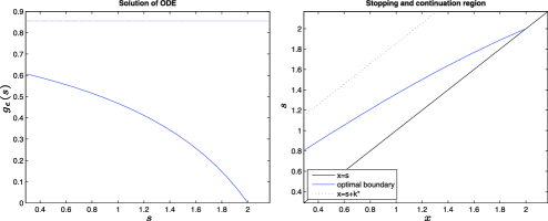
Figure 3: An illustration of $s\mapsto g_{\epsilon}(s)$ and the corresponding optimal boundary for $q=1.6$, $\epsilon=2$, $\sigma=0$, $\mu=3$, $a=3$ and $\rho=0.1$.

A first step towards more explicit solutions of (1) is looking at processes $X$ where explicit expressions for $W^{(q)}$ and $Z^{(q)}$ are available. In recent years various authors have found several processes whose scale functions are explicitly known (Example 1.3, Chapter 4 and Section 5.5 in KuzKypRiv , e.g.). Here, however, we would additionally like to find $g_{\epsilon}$ explicitly. To the best of our knowledge, we do not know of any examples where this is possible. One might instead try to solve (17) numerically, but this is not straightforward as there is no initial point to start a numerical scheme from and, moreover, the possibility of $g_{\epsilon}$ having infinite gradient at $\epsilon$ might lead to inaccuracies in the numerical scheme. Therefore, we follow a different route which avoids these difficulties. Instead of looking at $g_{\epsilon}$, we rather focus on its inverse

$$H(s)=\epsilon+\int_{0}^{s}\biggl{(}1-\frac{Z^{(q)}(\eta)}{qW^{(q)}(\eta)}\biggr{)}^{-1}\,d\eta,\qquad s\in\bigl{(}0,k^{*}\bigr{)},$$ (33)

where $k^{*}\in(0,\infty)$ is the unique root of $Z^{(q)}(z)-qW^{(q)}(z)=0$. It turns out that in some cases (including the Black–Scholes model) $H$ can be computed explicitly. Since $H$ is the inverse of $g_{\epsilon}$, plotting $(H(y),y),y\in(0,k^{*})$, yields visualisations of $s\mapsto g_{\epsilon}(s)$ for $s\in(-\infty,\epsilon)$; see Figures 3–5.

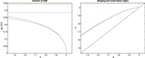
Figure 4: Left: a visualization of $s\mapsto g_{\epsilon}(s)$ for when $q=4$, $\epsilon=2$, $\sigma=1$ and $\mu=2$ (red) and $q=4$, $\epsilon=2$, $\sigma=1$, $\mu=2$, $a=3$ and $\rho=0.1$ (blue). Right: an illustration of the corresponding optimal boundaries.

Similarly, plotting $(H(y)-y,H(y)),y\in(0,k^{*})$, produces visualisations of the optimal stopping boundary in the $(x,s)$-plane; see Figures 3–5. Unfortunately, it is often the

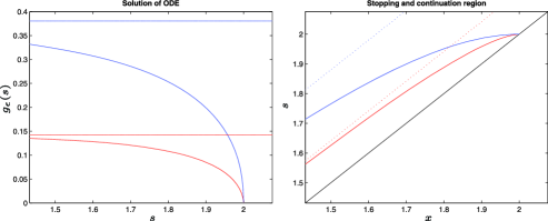
Figure 5: Left: a visualisation of $s\mapsto g_{\epsilon}(s)$ when $q=2$ and $\epsilon=2$, and $X$ is either a linear Brownian motion (blue curve, $\sigma=\sqrt{2}$, $\mu=0$) or an $\alpha$-stable process (red curve, $\alpha=1.6$).

case that we cannot compute the integral in (33) explicitly in which case one might use numerical integration in Matlab to obtain an approximation of the integral. The procedure just described is carried out below for different examples of $X$.

7.1 Brownian motion with drift and compound Poisson jumps

Consider the process

$$X_{t}=\sigma W_{t}+\mu t-\sum_{i=1}^{N_{t}}\xi_{i},\qquad t\geq 0,$$

where $\sigma>0$, $\mu\in\mathbb{R}$, $(W_{t})_{t\geq 0}$ is a standard Brownian motion, $(N_{t})_{t\geq 0}$ is a Poisson process with intensity $a>0$ and $\xi_{i}$ are i.i.d. random variables which are exponentially distributed with parameter $\rho>0$. The processes $(W_{t})_{t\geq 0}$ and $(N_{t})_{t\geq 0}$ as well as the sequence $(\xi_{i})_{i\in\mathbb{N}}$ are assumed to be mutually independent. The Laplace exponent of $X$ is given by

$$\psi(\theta)=\frac{\sigma^{2}}{2}\theta^{2}+\mu\theta-\frac{a\theta}{\rho+\theta},\qquad\theta\geq 0.$$

It is known (cf. Example 1.3 in KuzKypRiv and Section 8.2 of exitproblems ) that

$$W^{(q)}(x)=\frac{e^{\Phi(q)x}}{\psi^{\prime}(\Phi(q))}+\frac{e^{-\zeta_{1}x}}{\psi^{\prime}(-\zeta_{1})}+\frac{e^{-\zeta_{2}x}}{\psi^{\prime}(-\zeta_{2})},\qquad x\geq 0,$$ (34)

where $-\zeta_{2}<-\rho<-\zeta_{1}<0<\Phi(q)$ are the three real solutions of the equation $\psi(\theta)=q$, and that, for $x\geq 0$,

$$Z^{(q)}(x)=D_{1}e^{\Phi(q)x}+D_{2}e^{-\zeta_{1}x}+D_{3}e^{-\zeta_{2}x},$$ (35)

where $D_{1}=\frac{q}{\Phi(q)\psi^{\prime}(\Phi(q))}$, $D_{2}=\frac{q}{-\zeta_{1}\psi^{\prime}(-\zeta_{1})}$ and $D_{3}=\frac{q}{-\zeta_{2}\psi^{\prime}(-\zeta_{2})}$.

As a first example consider $\sigma=0$. In this case $\psi(\theta)=q$ reduces to a quadratic equation, and one can calculate explicitly

$$\zeta_{1} = \frac{1}{2\mu}\bigl{(}\sqrt{(a+q-\mu\rho)^{2}+4\mu q\rho}-(a+q-\mu\rho)\bigr{)},$$

$$\Phi(q) = \frac{1}{2\mu}\bigl{(}\sqrt{(a+q-\mu\rho)^{2}+4\mu q\rho}+(a+q-\mu\rho)\bigr{)}.$$

Moreover, it follows that

$$k^{*}=\frac{1}{\zeta_{1}+\phi(q)}\log\biggl{(}\frac{\Phi(q)\psi^{\prime}(\Phi(q))(\zeta_{1}+1)}{\zeta_{1}\psi^{\prime}(-\zeta_{1})(1-\Phi(q))}\biggr{)}.$$

Using elementary algebra and integration one finds, for $s\in(0,k^{*})$,

$$H(s) = \epsilon+\int_{0}^{s}\biggl{(}\frac{D_{1}\Phi(q)e^{(\Phi(q)+\zeta_{1})x}}{D_{1}(\Phi(q)-1)e^{(\Phi(q)+\zeta_{1})x}-D_{2}(\zeta_{1}+1)}\biggr{)}\,dx$$

$${}-\int_{0}^{s}\frac{D_{2}\zeta_{1}e^{-(\zeta_{1}+\Phi(q))x}}{D_{1}(\Phi(q)-1)-D_{2}(\zeta_{1}+1)e^{-(\zeta_{1}+\Phi(q))x}}\,dx$$

$$= \epsilon+\int_{0}^{s}\biggl{(}\frac{\Phi(q)e^{Ax}}{Be^{Ax}-CD}-\frac{\zeta_{1}e^{-Ax}}{C^{-1}B-De^{-Ax}}\biggr{)}\,dx$$

$$= \epsilon+\frac{\Phi(q)}{AB}\log\biggl{|}\frac{Be^{As}-CD}{B-CD}\biggr{|}-\frac{\zeta_{1}}{AD}\log\biggl{|}\frac{B-CDe^{-As}}{B-CD}\biggr{|},$$

where $A:=\zeta_{1}+\Phi(q),B:=\Phi(q)-1,C:=\frac{\Phi(q)\psi^{\prime}(\Phi(q))}{-\zeta_{1}\psi^{\prime}(-\zeta_{1})}$ and $D:=\zeta_{1}+1$. An example for a certain choice of parameters is given in Figure 3.

Next, assume $\sigma>0$ and $\rho=\infty$; that is, $X$ is a linear Brownian motion. In particular, this includes the Black–Scholes model. Again, as explained in Example 1.3 of KuzKypRiv , the equation $\psi(\theta)=q$ reduces to a quadratic equation and $\zeta_{1}=\delta-\gamma$ and $\Phi(q)=\delta+\gamma$, where

$$\gamma:=-\frac{\mu}{\sigma^{2}}\quad\mbox{and}\quad\delta:=\frac{1}{\sigma^{2}}\sqrt{\mu^{2}+2q\sigma^{2}}.$$

Furthermore, (34) and (35) may be rewritten on $x\geq 0$ as

$$W^{(q)}(x) = \frac{2}{\sigma^{2}\delta}e^{\gamma x}\sinh(\delta x)\quad\mbox{and}$$

$$Z^{(q)}(x) = e^{\gamma x}\cosh(\delta x)-\frac{\gamma}{\delta}e^{\gamma x}\sinh(\delta x)$$

and one can compute

$$k^{*}=\frac{1}{\Phi(q)+\zeta_{1}}\log\biggl{(}\frac{1+\zeta_{1}^{-1}}{1-\Phi(q)^{-1}}\biggr{)}.$$ (37)

Using elementary algebra in the first and formula 2.447.1 of gradshteyn in the second equality one obtains, for $s\in(0,k^{*})$,

$$H(s) = \epsilon+\frac{2q}{\sigma^{2}\delta}\int_{0}^{s\delta}\frac{\sinh(x)}{(2q/\sigma^{2}+\gamma)\cosh(x)-\delta\sinh(x)}\,dx$$

$$= \epsilon+\frac{2q}{\sigma^{2}\delta(F^{2}-\delta^{2})}\biggl{(}F\delta s-\delta\log\biggl{|}\frac{\sinh(\tanh^{-1}(-\delta F^{-1}))}{\sinh(\delta s+\tanh^{-1}(-\delta F^{-1}))}\biggr{|}\biggr{)},$$

where $F:=2q/\sigma^{2}+\gamma$. An example for a certain parameter choice is provided in Figure 4.

In the next example we combine the first example with the second one. More precisely, suppose that $\sigma>$ and $\rho\in(0,\infty)$, that is, a linear Brownian motion with exponential jumps. In this case we are unable to compute $k^{*}$ and $H$ explicitly. We therefore find $k^{*}$ numerically and use numerical integration to obtain an approximation of $k^{*}$ and $H$, respectively; see Figure 4.

7.2 Stable jumps

Suppose that $X$ is an $\alpha$-stable process, where $\alpha\in(1,2]$ with Laplace exponent $\psi(\theta)=\theta^{\alpha},\theta\geq 0$. It is known (cf. Example 4.17 of KuzKypRiv and Section 8.3 of exitproblems ) that, for $x\geq 0$,

$$W^{(q)}(x)=x^{\alpha-1}E_{\alpha,\alpha}\bigl{(}qx^{\alpha}\bigr{)}\quad\mbox{and}\quad Z^{(q)}(x)=E_{\alpha,1}\bigl{(}qx^{\alpha}\bigr{)},$$

where $E_{\alpha,\beta}$ is the two-parameter Mittag–Leffler function which is defined for $\alpha>0,\beta>0$ as

$$E_{\alpha,\beta}(x)=\sum_{n=0}^{\infty}\frac{x^{n}}{\Gamma(\alpha n+\beta)}.$$

Again, using numerical integration and a Matlab function that computes the Mittag–Leffler function (cf. mittaglefflerfunction ) one may approximate $k^{*}$ and $H$, respectively; see Figure 5. Additionally, we have computed the value function for a choice of parameters (Figure 6).

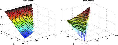
Figure 6: Left: a visualisation of $V_{\epsilon}^{*}(x,s)$ when $X$ is $\alpha$-stable with parameter choice $q=3$, $\epsilon=2$ and $\alpha=1.6$. Right: an illustration of the difference between $V_{\epsilon_{2}}^{*}(x,s)$ (darker surface) and $V^{*}_{\epsilon_{1},\epsilon_{2}}(x,s)$ (lighter surface) on $C^{*}_{I,\epsilon_{1},\epsilon_{2}}$ for the same $X$ and same parameters as on the left. In this case $A\approx 1.63$, where $A$ is formally defined in Section 4.2.

If one considers a lower cap $\epsilon_{1}$ and an upper cap $\epsilon_{2}$, then the only thing that changes for the optimal boundary is that one has to include an additional vertical line at the value of the lower cap $\epsilon_{1}$. However, introducing a lower cap will make a difference, that is, the value functions $V_{\epsilon_{2}}^{*}(x,s)$ and $V^{*}_{\epsilon_{1},\epsilon_{2}}(x,s)$ will be different for $(x,s)\in C^{*}_{I,\epsilon_{1},\epsilon_{2}}$; see Theorems 4.2 and 4.4. Exploiting the fact that $H$ is the inverse of $g_{\epsilon_{2}}$ in a similar way as above, one may also obtain numerical approximations of the value functions $V^{*}_{\epsilon_{2}}(x,s)$ and $V^{*}_{\epsilon_{1},\epsilon_{2}}(x,s)$; see Figure 6.

7.3 Maximum process with lower cap only

Assume the same setting as in the second example above, that is, $X_{t}=\sigma W_{t}+\mu t$. The scale functions and $k^{*}$ are given by (7.1) and (37), respectively. If we suppose that there is a lower cap $\epsilon_{1}\in\mathbb{R}$ and no upper cap ($\epsilon_{2}=\infty$), then Corollary 4.5 can be rewritten more explicitly as follows.

Lemma 7.1

The $V^{*}$ and $U_{\epsilon_{1},\infty}$ part of the optimal value function $V_{\epsilon_{1},\infty}^{*}$ are given by

$$V^{*}(x,s)=\frac{1}{\Phi(q)+\zeta_{1}}\biggl{(}\Phi(q)\biggl{(}\frac{e^{x}}{e^{s-k^{*}}}\biggr{)}^{-\zeta_{1}}+\zeta_{1}\biggl{(}\frac{e^{x}}{e^{s-k^{*}}}\biggr{)}^{\Phi(q)}\biggr{)}$$

and

$$U_{\epsilon_{1},\infty}(x,s) = \biggl{(}\frac{e^{x}}{e^{\epsilon_{1}}}\biggr{)}^{-\zeta_{1}}\biggl{[}-\frac{e^{\epsilon_{1}}}{\beta}\biggl{(}\int_{\beta(s-\epsilon_{1})}^{\beta k^{*}}\frac{e^{u(1+y)}}{e^{u}-1}\,du-e^{k^{*}\Phi(q)}\biggr{)}\biggr{]}$$

$${}+\biggl{(}\frac{e^{x}}{e^{\epsilon_{1}}}\biggr{)}^{\Phi(q)}\biggl{[}\frac{e^{\epsilon_{1}}}{\beta}\biggl{(}\int_{\beta(s-\epsilon_{1})}^{\beta k^{*}}\frac{e^{uy}}{e^{u}-1}\,du-e^{-k^{*}\zeta_{1}}\biggr{)}\biggr{]},$$

where $\beta=\Phi(q)+\zeta_{1}=2\delta$ and $y=\beta^{-1}$.

The proof of this result is a lengthy computation provided in Appendix B. Finally, if we set $\epsilon_{1}=\epsilon$, $\mu=r-\sigma^{2}/2$ for some $r\geq 0$ and $q=\lambda+r$ for some $\lambda>0$ we recover Theorem 3.1 of abarrierversion .

Appendix A Complementary results on the infinitesimal generator of $X$

In this section we provide some results concerning the infinitesimal generator of $X$ when applied to the scale function $Z^{(q)}$.

First assume that $X$ is of unbounded variation, and define an operator $(\Gamma,\mathcal{D}(\Gamma))$ as follows. $\mathcal{D}(\Gamma)$ stands for the family of functions $f\in C^{2}(0,\infty)$ such that the integral

$$\int_{(-\infty,0)}\bigl{(}f(x+y)-f(x)-yf^{\prime}(x)1_{\{y\geq-1\}}\bigr{)}\Pi(dy)$$

is absolutely convergent for all $x>0$. For any $f\in\mathcal{D}(\Gamma)$, we define the function $\Gamma f\dvtx(0,\infty)\rightarrow\mathbb{R}$ by

$$\Gamma f(x) = -\gamma f^{\prime}(x)+\frac{\sigma^{2}}{2}f^{\prime\prime}(x)$$

$${}+\int_{(-\infty,0)}\bigl{(}f(x+y)-f(x)-yf^{\prime}(x)1_{\{y\geq-1\}}\bigr{)}\Pi(dy).$$

Similarly, if $X$ is of bounded variation, then $\mathcal{D}(\Gamma)$ stands for the family of $f\in C^{1}(0,\infty)$ such that the integral

$$\int_{(-\infty,0)}\bigl{(}f(x+y)-f(x)\bigr{)}\Pi(dy)$$

is absolutely convergent for all $x>0$, and for $f\in\mathcal{D}(\Gamma)$, we define the function $\Gamma f\dvtx(0,\infty)\rightarrow\mathbb{R}$ by

$$\Gamma f(x)=\mathtt{d}f^{\prime}(x)+\int_{(-\infty,0)}\bigl{(}f(x+y)-f(x)\bigr{)}\Pi(dy).$$

In the sequel it should always be clear from the context in which of the two cases we are and therefore there should be no ambiguity when writing $\mathcal{D}(\Gamma)$ and $\Gamma$.

Lemma A.1

We have that $Z^{(q)}\in\mathcal{D}(\Gamma)$ and the function $x\mapsto\Gamma Z^{(q)}(x)$ is continuous on $(0,\infty)$.

We prove the unbounded and bounded variation case separately.

Unbounded variation: To show that $Z^{(q)}\in\mathcal{D}(\Gamma)$ it is enough to check that the integral part of $\Gamma Z^{(q)}$ is absolutely convergent since $Z^{(q)}\in C^{2}(0,\infty)$. Fix $x>0$ and write the integral part of $\Gamma Z^{(q)}$ as

$$\int_{(-\infty,-\delta)}\bigl{|}Z^{(q)}(x+y)-Z^{(q)}(x)-yZ^{(q)\prime}(x)1_{\{y\geq-1\}}\bigr{|}\Pi(dy)$$

$$\qquad{}+\int_{(-\delta,0)}\bigl{|}Z^{(q)}(x+y)-Z^{(q)}(x)-yZ^{(q)\prime}(x)1_{\{y\geq-1\}}\bigr{|}\Pi(dy),$$

where the value $\delta=\delta(x)\in(0,1)$ is chosen such that $x-\delta>0$. For $y\in(-\infty,-\delta)$ the monotonicity of $Z^{(q)}$ implies

$$\bigl{|}Z^{(q)}(x+y)-Z^{(q)}(x)-yZ^{(q)\prime}(x)1_{\{y\geq-1\}}\bigr{|}\leq 2Z^{(q)}(x)+Z^{(q)\prime}(x)$$ (38)

and for $y\in(-\delta,0)$, using the mean value theorem, we have

$$\bigl{|}Z^{(q)}(x+y)-Z^{(q)}(x)-yZ^{(q)\prime}(x)\bigr{|}$$

$$\qquad=q|y|\bigl{|}W^{(q)}\bigl{(}\xi(y)\bigr{)}-W^{(q)}(x)\bigr{|}\qquad\mbox{where $\xi(y)\in(x+y,x)$}$$

(39)

$$\qquad=q|y|\biggl{|}\int_{\xi(y)}^{x}W^{(q)\prime}(z)\,dz\biggr{|}$$

$$\qquad\leq qy^{2}\sup_{z\in[x-\delta,x]}W^{(q)\prime}(z).$$

Using these two estimates and defining $C(\delta)=\int_{(-\delta,0)}y^{2}\Pi(dy)<\infty$, we see that

$$\int_{(-\infty,0)}\bigl{|}Z^{(q)}(x+y)-Z^{(q)}(x)-yZ^{(q)\prime}(x)1_{\{y\geq-1\}}\bigr{|}\Pi(dy)$$

$$\qquad\leq\bigl{(}2Z^{(q)}(x)+Z^{(q)\prime}(x)\bigr{)}\Pi(-\infty,-\delta)+qC(\delta)\sup_{z\in[x-\delta,x]}W^{(q)\prime}(z)<\infty.$$

For continuity, let $x>0$ and choose $\delta=\delta(x)\in(0,1)$ such that $x-2\delta>0$ as well as a sequence $(x_{n})_{n\in\mathbb{N}}$ converging to $x$. Moreover, let $n_{0}\in\mathbb{N}$ such that for all $n\geq n_{0}$ we have $|x_{n}-x|<\delta$. In particular, it holds that $x_{n}-\delta>0$ for $n\geq n_{0}$ and hence, using the estimates in (38) and (A), we have for all $n\geq n_{0}$

$$\bigl{|}Z^{(q)}(x_{n}+y)-Z^{(q)}(x_{n})-yZ^{(q)\prime}(x_{n})1_{\{y\geq-1\}}\bigr{|}$$

$$\qquad\leq qy^{2}\sup_{z\in[x_{n}-\delta,x_{n}]}W^{(q)\prime}(z)1_{\{y\geq-\delta\}}+\bigl{(}2Z^{(q)}(x_{n})+Z^{(q)\prime}(x_{n})\bigr{)}1_{\{y<-\delta\}}$$

$$\qquad\leq qy^{2}\sup_{z\in[x-2\delta,x+\delta]}W^{(q)\prime}(z)1_{\{y\geq-\delta\}}+\bigl{(}2Z^{(q)}(x+\delta)+Z^{(q)\prime}(x+\delta)\bigr{)}1_{\{y<-\delta\}}.$$

Since the last term is $\Pi$-integrable, the continuity assertion follows by dominated convergence and the fact that $Z^{(q)}\in C^{2}(0,\infty)$.

Bounded variation: To show that $Z^{(q)}\in\mathcal{D}(\Gamma)$ it is enough to show that the integral part of $\Gamma Z^{(q)}$ is absolutely convergent since $Z^{(q)}\in C^{1}(0,\infty)$. Using the monotonicity and the definition of $Z^{(q)}$, it is easy to see that for fixed $x>0$,

$$\int_{(-\infty,0)}\bigl{|}Z^{(q)}(x+y)-Z^{(q)}(x)\bigr{|}\Pi(dy)$$

$$\qquad\leq 2Z^{(q)}(x)\Pi(-\infty,-1)+qW^{(q)}(x)\int_{(-1,0)}|y|\Pi(dy)<\infty.$$

The continuity assertion follows in a straightforward manner from dominated convergence and the fact that $Z^{(q)}\in C^{1}(0,\infty)$.

Appendix B A lengthy computation

Proof of Lemma 7.1 The first part is a short calculation using the definition of $\gamma$, $\delta$, $\zeta_{1}$, $\Phi(q)$ and that $\cosh(z)=\frac{e^{z}+e^{-z}}{2}$ and $\sinh(z)=\frac{e^{z}-e^{-z}}{2}$. As for the second part, recall that, for $(x,s)\in C^{*}_{I}\cup D^{*}_{I}$,

$$U_{\epsilon_{1},\infty}(x,s)=e^{s}Z^{(q)}(x-\epsilon_{1})+e^{\epsilon_{1}}W^{(q)}(x-\epsilon_{1})\int_{s-\epsilon_{1}}^{k^{*}}e^{t}\frac{Z^{(q)}(t)}{W^{(q)}(t)}\,dt.$$

It is easy to see that

$$e^{t}\frac{Z^{(q)}(t)}{W^{(q)}(t)}=e^{t}\frac{\delta\sigma^{2}}{2}\biggl{(}\frac{1}{1-e^{-2\delta t}}+\frac{1}{e^{2\delta t}-1}\biggr{)}-e^{t}\frac{\gamma\sigma^{2}}{2},$$

which, after a change of variables, gives

$$\int_{s-\epsilon_{1}}^{k^{*}}e^{t}\frac{Z^{(q)}(t)}{W^{(q)}(t)}\,dt = \frac{\sigma^{2}}{4}\biggl{(}\int_{\beta(s-\epsilon_{1})}^{\beta k^{*}}\frac{e^{u(1+y)}}{e^{u}-1}\,du+\int_{\beta(s-\epsilon_{1})}^{\beta k^{*}}\frac{e^{uy}}{e^{u}-1}\,du\biggr{)}$$

$${}+\frac{\gamma\sigma^{2}}{2}\bigl{(}e^{s-\epsilon_{1}}-e^{k^{*}}\bigr{)},$$

where $\beta=\Phi(q)+\zeta_{1}=2\delta$ and $y=\beta^{-1}$. Denote the first integral on the right-hand side $I_{1}$ and the second integral $I_{2}$. After some algebra one sees that $U_{\epsilon_{1},\infty}(x,s)$ equals

$$\frac{e^{s}}{2}\bigl{(}e^{\Phi(q)(x-\epsilon_{1})}+e^{-\zeta_{1}(x-\epsilon_{1})}\bigr{)}-\frac{e^{\epsilon_{1}+k^{*}}\gamma}{\beta}\bigl{(}e^{\Phi(q)(x-\epsilon_{1})}-e^{-\zeta(x-\epsilon_{1})}\bigr{)}$$

$$\qquad{}-\frac{e^{\epsilon_{1}}}{2\beta}e^{-\zeta_{1}(x-\epsilon_{1})}I_{1}+\frac{e^{\epsilon_{1}}}{2\beta}e^{\Phi(q)(x-\epsilon_{1})}I_{2}$$

$$\qquad{}+\frac{e^{\epsilon_{1}}}{2\beta}e^{\Phi(q)(x-\epsilon_{1})}I_{1}-\frac{e^{\epsilon_{1}}}{2\beta}e^{-\zeta_{1}(x-\epsilon_{1})}I_{2}.$$

Next, note that the last line in (B) can be rewritten as

$$\frac{e^{\epsilon_{1}}}{2\beta}\bigl{(}e^{\Phi(q)(x-\epsilon_{1})}+e^{-\zeta_{1}(x-\epsilon_{1})}\bigr{)}(I_{1}-I_{2})-\frac{e^{\epsilon_{1}}}{2\beta}e^{-\zeta_{1}(x-\epsilon_{1})}I_{1}+\frac{e^{\epsilon_{1}}}{2\beta}e^{\Phi(q)(x-\epsilon_{1})}I_{2}$$

$$\qquad=\frac{e^{\epsilon_{1}}}{2}\bigl{(}e^{\Phi(q)(x-\epsilon_{1})}+e^{-\zeta_{1}(x-\epsilon_{1})}\bigr{)}\bigl{(}e^{k^{*}}-e^{s-\epsilon_{1}}\bigr{)}$$

$$\qquad\quad{}-\frac{e^{\epsilon_{1}}}{2\beta}e^{-\zeta_{1}(x-\epsilon_{1})}I_{1}+\frac{e^{\epsilon_{1}}}{2\beta}e^{\Phi(q)(x-\epsilon_{1})}I_{2},$$

where the equality follows from evaluating $I_{1}-I_{2}$. Plugging this into (B) and simplifying yields

$$U_{\epsilon_{1},\infty}(x,s) = -e^{-\zeta_{1}(x-\epsilon_{1})}e^{\epsilon_{1}}\beta^{-1}I_{1}+e^{\Phi(q)(x-\epsilon_{1})}e^{\epsilon_{1}}\beta^{-1}I_{2}$$

$${}+e^{\epsilon_{1}+\Phi(q)(x-\epsilon_{1})}e^{k^{*}}\beta^{-1}\zeta_{1}+e^{\epsilon_{1}-\zeta_{1}(x-\epsilon_{1})}e^{k^{*}}\beta^{-1}\Phi(q).$$

Rearranging the terms completes the proof.

References

- (1) {barticle}[mr] \bauthor\bsnmAlili, \bfnmL.\binitsL. and \bauthor\bsnmKyprianou, \bfnmA. E.\binitsA. E. (\byear2005). \btitleSome remarks on first passage of Lévy processes, the American put and pasting principles. \bjournalAnn. Appl. Probab. \bvolume15 \bpages2062–2080. \biddoi=10.1214/105051605000000377, issn=1050-5164, mr=2152253 \bptokimsref \endbibitem
- (2) {barticle}[mr] \bauthor\bsnmAvram, \bfnmF.\binitsF., \bauthor\bsnmKyprianou, \bfnmA. E.\binitsA. E. and \bauthor\bsnmPistorius, \bfnmM. R.\binitsM. R. (\byear2004). \btitleExit problems for spectrally negative Lévy processes and applications to (Canadized) Russian options. \bjournalAnn. Appl. Probab. \bvolume14 \bpages215–238. \biddoi=10.1214/aoap/1075828052, issn=1050-5164, mr=2023021 \bptokimsref \endbibitem
- (3) {barticle}[mr] \bauthor\bsnmBaurdoux, \bfnmE. J.\binitsE. J. and \bauthor\bsnmKyprianou, \bfnmA. E.\binitsA. E. (\byear2009). \btitleThe Shepp–Shiryaev stochastic game driven by a spectrally negative Lévy process. \bjournalTheory Probab. Appl. \bvolume53 \bpages481–499. \bptokimsref \endbibitem
- (4) {bbook}[mr] \bauthor\bsnmBertoin, \bfnmJean\binitsJ. (\byear1996). \btitleLévy Processes. \bseriesCambridge Tracts in Mathematics \bvolume121. \bpublisherCambridge Univ. Press, \blocationCambridge. \bidmr=1406564 \bptokimsref \endbibitem
- (5) {bbook}[mr] \bauthor\bsnmBichteler, \bfnmKlaus\binitsK. (\byear2002). \btitleStochastic Integration with Jumps. \bseriesEncyclopedia of Mathematics and Its Applications \bvolume89. \bpublisherCambridge Univ. Press, \blocationCambridge. \biddoi=10.1017/CBO9780511549878, mr=1906715 \bptokimsref \endbibitem
- (6) {barticle}[auto:STB—2013/01/29—08:09:18] \bauthor\bsnmCarr, \bfnmP.\binitsP. and \bauthor\bsnmWu, \bfnmL.\binitsL. (\byear2003). \btitleThe finite moment log stable process and option pricing. \bjournalJ. Finance \bvolume58 \bpages753–778. \bptokimsref \endbibitem
- (7) {barticle}[mr] \bauthor\bsnmChan, \bfnmTerence\binitsT. (\byear1999). \btitlePricing contingent claims on stocks driven by Lévy processes. \bjournalAnn. Appl. Probab. \bvolume9 \bpages504–528. \biddoi=10.1214/aoap/1029962753, issn=1050-5164, mr=1687394 \bptokimsref \endbibitem
- (8) {bbook}[mr] \bauthor\bsnmGradshteyn, \bfnmI. S.\binitsI. S. and \bauthor\bsnmRyzhik, \bfnmI. M.\binitsI. M. (\byear2007). \btitleTable of Integrals, Series, and Products, \bedition7th ed. \bpublisherElsevier, \blocationAmsterdam. \bidmr=2360010 \bptokimsref \endbibitem
- (9) {bmisc}[auto:STB—2013/01/29—08:09:18] \bauthor\bsnmKuznetsov, \bfnmA.\binitsA., \bauthor\bsnmKyprianou, \bfnmA. E.\binitsA. E. and \bauthor\bsnmRivero, \bfnmV.\binitsV. (\byear2011). \bhowpublishedThe theory of scale functions for spectrally negative Lévy processes. Available at arXiv:\arxivurl1104.1280v1 [math.PR]. \bptokimsref \endbibitem
- (10) {bbook}[mr] \bauthor\bsnmKyprianou, \bfnmAndreas E.\binitsA. E. (\byear2006). \btitleIntroductory Lectures on Fluctuations of Lévy Processes with Applications. \bpublisherSpringer, \blocationBerlin. \bidmr=2250061 \bptokimsref \endbibitem
- (11) {bmisc}[auto:STB—2013/01/29—08:09:18] \bauthor\bsnmMadan, \bfnmD. B.\binitsD. B. and \bauthor\bsnmSchoutens, \bfnmW.\binitsW. (\byear2008). \bhowpublishedBreak on through to the single side. J. Credit Risk 4(3). \bptokimsref \endbibitem
- (12) {barticle}[auto:STB—2013/01/29—08:09:18] \bauthor\bsnmMerton, \bfnmR. C.\binitsR. C. (\byear1969). \btitleLifetime portfolio selection under uncertainty: The continuous-time case. \bjournalRev. Econ. Stat. \bvolume1 \bpages247–257. \bptokimsref \endbibitem
- (13) {barticle}[auto:STB—2013/01/29—08:09:18] \bauthor\bsnmMikalevich, \bfnmV. S.\binitsV. S. (\byear1958). \btitleBaysian choice between two hypotheses for the mean value of a normal process. \bjournalVisn. Kiiv. Univ. Ser. Fiz.-Mat. Nauki \bvolume1 \bpages101–104. \bptokimsref \endbibitem
- (14) {barticle}[mr] \bauthor\bsnmPeskir, \bfnmGoran\binitsG. (\byear1998). \btitleOptimal stopping of the maximum process: The maximality principle. \bjournalAnn. Probab. \bvolume26 \bpages1614–1640. \biddoi=10.1214/aop/1022855875, issn=0091-1798, mr=1675047 \bptokimsref \endbibitem
- (15) {bbook}[mr] \bauthor\bsnmPeskir, \bfnmGoran\binitsG. and \bauthor\bsnmShiryaev, \bfnmAlbert\binitsA. (\byear2006). \btitleOptimal Stopping and Free-Boundary Problems. \bpublisherBirkhäuser, \blocationBasel. \bidmr=2256030 \bptokimsref \endbibitem
- (16) {barticle}[mr] \bauthor\bsnmPeskir, \bfnmG.\binitsG. and \bauthor\bsnmShiryaev, \bfnmA. N.\binitsA. N. (\byear2000). \btitleSequential testing problems for Poisson processes. \bjournalAnn. Statist. \bvolume28 \bpages837–859. \biddoi=10.1214/aos/1015952000, issn=0090-5364, mr=1792789 \bptokimsref \endbibitem
- (17) {barticle}[mr] \bauthor\bsnmPistorius, \bfnmM. R.\binitsM. R. (\byear2004). \btitleOn exit and ergodicity of the spectrally one-sided Lévy process reflected at its infimum. \bjournalJ. Theoret. Probab. \bvolume17 \bpages183–220. \biddoi=10.1023/B:JOTP.0000020481.14371.37, issn=0894-9840, mr=2054585 \bptokimsref \endbibitem
- (18) {bmisc}[auto:STB—2013/01/29—08:09:18] \bauthor\bsnmPodlubny, \bfnmI.\binitsI. (\byear2012). \bhowpublishedMittag-Leffler function [Matlab code]. Available at http://www.mathworks.com/matlabcentral/fileexchange/8738. \bptokimsref \endbibitem
- (19) {bbook}[mr] \bauthor\bsnmProtter, \bfnmPhilip E.\binitsP. E. (\byear2005). \btitleStochastic Integration and Differential Equations, \bedition2nd ed. \bseriesStochastic Modelling and Applied Probability \bvolume21. \bpublisherSpringer, \blocationBerlin. \bidmr=2273672 \bptokimsref \endbibitem
- (20) {barticle}[mr] \bauthor\bsnmShepp, \bfnmLarry\binitsL. and \bauthor\bsnmShiryaev, \bfnmA. N.\binitsA. N. (\byear1993). \btitleThe Russian option: Reduced regret. \bjournalAnn. Appl. Probab. \bvolume3 \bpages631–640. \bidissn=1050-5164, mr=1233617 \bptokimsref \endbibitem
- (21) {barticle}[auto:STB—2013/01/29—08:09:18] \bauthor\bsnmShepp, \bfnmL. A.\binitsL. A. and \bauthor\bsnmShiryaev, \bfnmA. N.\binitsA. N. (\byear1993). \btitleA new look at pricing of the “Russian option.” \bjournalTheory Probab. Appl. \bvolume39 \bpages103–119. \bptokimsref \endbibitem
- (22) {bincollection}[mr] \bauthor\bsnmShepp, \bfnmL. A.\binitsL. A., \bauthor\bsnmShiryaev, \bfnmAlbert N.\binitsA. N. and \bauthor\bsnmSulem, \bfnmA.\binitsA. (\byear2002). \btitleA barrier version of the Russian option. In \bbooktitleAdvances in Finance and Stochastics \bpages271–284. \bpublisherSpringer, \blocationBerlin. \bptokimsref \endbibitem
- (23) {bbook}[mr] \bauthor\bsnmShiryaev, \bfnmAlbert N.\binitsA. N. (\byear1999). \btitleEssentials of Stochastic Finance: Facts, Models, Theory. \bseriesAdvanced Series on Statistical Science & Applied Probability \bvolume3. \bpublisherWorld Scientific, \blocationRiver Edge, NJ. \biddoi=10.1142/9789812385192, mr=1695318 \bptokimsref \endbibitem