Accurate determination of the Gaussian transition in spin-1 chains with single-ion anisotropy

Abstract

The Gaussian transition in the spin-one Heisenberg chain with single-ion anisotropy is extremely difficult to treat, both analytically and numerically. We introduce an improved DMRG procedure with strict error control, which we use to access very large systems. By considering the bulk entropy, we determine the Gaussian transition point to 4-digit accuracy, $D_{c}/J=0.96845(8)$, resolving a long-standing debate in quantum magnetism. With this value, we obtain high-precision data for the critical behavior of quantities including the ground-state energy, gap, and transverse string-order parameter, and for the critical exponent, $\nu=1.472(2)$. Applying our improved technique at $J_{z}=0.5$ highlights essential differences in critical behavior along the Gaussian transition line.

The Gaussian transition appears in several fields of quantum physics and statistical mechanics. The equivalence between surface-roughening transitions in classical two-dimensional (2D) models and quantum phase transitions in spin chains was introduced in Ref. rls , and their rich phase diagrams investigated at length in Ref. rdnr . Characterized by continuously variable exponents, the Gaussian transition differs significantly both from regular phase transitions and from those of Kosterlitz-Thouless (KT) type. These differences complicate both analytical and numerical approaches to a complete and accurate description of rough surfaces and quantum spin chains.

The $S=1$ Heisenberg chain is one of the fundamental models in quantum magnetism. It formed the basis of Haldane’s conjecture haldane for a finite gap in antiferromagnetic chains with integer spin, as opposed to the gapless spectrum of half-odd-integer cases. Numerically, quantum spin chains are important test-cases for any computational technique, and Haldane’s prediction has been verified by a range of methods with increasing accuracy blote ; white . Experimentally, while the “Haldane gap” has been found in the excitation spectra of many systems rybno , most known $S=1$ chains, including NENP rnenp , NINAZ rninaz , and NDMAP rndmap , are organic Ni materials with significant single-ion anisotropies. Analytical approaches to the Gaussian transition driven by this term are complicated by the lack of a suitable effective field theory rs , and its broad nature makes all numerical techniques difficult to apply. Many authors have considered this transition, producing occasionally contradictory results rbjk ; rst ; rgjl ; rtnk ; rchs ; rdeor ; rthcy ; runk ; raho .

In this Letter we resolve the problem of the Gaussian transition in the $S$ = 1 chain with single-ion anisotropy. We exploit the fact that this transition is a gapless point between two gapped phases, whence the entropy exhibits a sharp peak. We introduce an improved density-matrix renormalization-group (DMRG) approach with systematic error control, allowing high-precision calculations at system sizes up to $L=20000$, which automatically eliminate the end-spin entropy. We determine the critical point with very high accuracy, and thereby deduce the critical behavior of several quantities at different points on the Gaussian transition line.

The general form of the model is

$${\cal H}\!=\!\mbox{$\sum^{L}_{i=1}$}\!J(S^{x}_{i}S^{x}_{i+1}\!+\!S^{y}_{i}S^{y}_{i+1})+J_{z}S^{z}_{i}S^{z}_{i+1}+D\left(S^{z}_{i}\right)^{2}\!\!$$ (1)

where $J_{z}$ interpolates between XY and Ising spins, $D$ is the single-ion anisotropy, and $L$ the length of the chain. The full parameter space of $(D,J_{z})$ contains Néel, Haldane, large-$D$, ferromagnetic, and two XY phases. In classical planar surface, or “solid-on-solid,” models, the Néel and large-$D$ phases are different “flat” phases, the Haldane phase is “rough,” and the Gaussian transition is of “preroughening” type. These are the three phases of the $S=1$ Heisenberg chain ($J_{z}=1$) as $D$ is varied. While the Néel phase possesses $Z_{2}$ symmetry and the Haldane phase an incomplete $Z_{2}\times Z_{2}$ symmetry, the large-$D$ phase has no remaining symmetries. The Gaussian transition is a line in the $(D,J_{z})$ plane, on which the excitations are gapless. This line is well described by a conformal field theory (CFT) cft , and has been analyzed in a number of studies rchs ; rdeor ; rthcy ; runk , but none has achieved the numerical precision required for a consistent discussion of the critical behavior across the transition.

DMRG is the most efficient and accurate numerical technique for 1D systems white . Anticipating the need for both large system sizes and extreme precision, we begin by introducing an improved DMRG technique. In the conventional scheme, the absolute (coupled round-off and truncation) error increases systematically with $L$, and this accumulated error has a strong effect on the relability of the computation, possibly even disguising the critical behavior in a quantum many-body system. We fix the round-off error by renormalizing the lowest eigenvalue of Hamiltonian to remain of order 1, thereby obtaining a very significant reduction in the truncation error for large systems. In the DMRG iteration, we replace the original Hamiltonian matrix $H(m,L)$, for chains of $L$ sites with $m$ kept states, by $H(m,L)-[\varepsilon_{1}(m,L-2)-\delta]$, where $\varepsilon_{1}(m,L-2)$ is the lowest eigenvalue of $H(m,L-2)$ and $\delta$ is a constant chosen such that $\varepsilon_{1}(m,L)\sim O(1)$. Here we use $\delta/J=1$ throughout. While the (extensive) total energy of the ground state, $E_{g}(m,L)$, can be reconstructed by summation, its (intensive) average value per site is determined directly and self-consistently as $e_{g}(m,L)=[\varepsilon_{1}(m,L)-\delta]/2$. Similarly, for the first excited state $e_{f}(m,L)=[\varepsilon_{2}(m,L)-\epsilon_{2}(m,L-2)]/2+e_{g}(m,L)$, where $\varepsilon_{2}(m,L)$ is the second-lowest eigenvalue of $H(m,L)$.

The gap in our method is given simply by $\Delta(m,L)=\varepsilon_{2}(m,L)-\varepsilon_{1}(m,L)$. Its general expression is

$$\Delta(m,\!L)\!=\![e_{f}(\!m\!)-e_{g}(\!m\!)]L+\Delta(\!m\!)+\!\mbox{$\sum^{\infty}_{n=1}$}\!\frac{\alpha_{n}(\!m\!)}{L^{n}},$$ (2)

where $e_{g}(m)$ and $e_{f}(m)$ are the intensive energies of the ground and first excited states for infinite $L$, and become equal for infinite $m$. In the polynomial expansion of contributions at higher order in $1/L$, the $n=1$ term arises from truncation errors and open boundary conditions (OBCs), while the $n=2$ term has contributions from fluctuations at the quadratic band minimum. Here we calculate the energies in the linear term independently by extrapolation. Subtracting these gives a gap function $\Delta(m,L)$ that decreases monotonically with increasing $L$. A second polynomial fit of $\Delta(m)$ allows its extrapolation to infinite $m$ to obtain the true gap.

Sharing its foundations with quantum information theory, the DMRG method is ideally suited to discussions of entropy and entanglement. The von Neumann entropy, ${\cal S}(m,L)=-{\rm Tr}\rho(m,L)\ln\rho(m,L)$, is readily computed from the reduced density matrix, which we obtain to high accuracy throughout our calculations with the renormalized Hamiltonian. The entropy obeys an area law except in critical regimes, where it depends logarithmically on $L$ rcc . This extremum in entropy is an excellent indicator of a (gapless) critical point between two gapped phases.

Before analyzing the entropy, we discuss the special and remarkable feature of the $S=1$ Heisenberg chain, that free $S=1/2$ entities are found at a chain end, both in theory and in experiment effectivespin . In the Haldane phase with OBCs, the two free end-spins can be described by $\hat{H}_{\rm eff}=J_{\rm eff}{\vec{S}}_{L}\cdot{\vec{S}}_{R}$ white , where the effective coupling $J_{\rm eff}>0$ falls exponentially with $L$. In the Hilbert space $S^{\rm tot}_{z}=0$, the two spins are maximally entangled with entropy $\ln 2$, while for $S^{\rm tot}_{z}=1$ they are unentangled. The additional truncation error due to this edge-entropy contribution causes significant computational difficulties. In Fig. 1(a) we find a $\ln 2$ drop in the ground-state entropy ${\cal S}(L)$ in the Hilbert space $S^{\rm tot}_{z}=0$ when the chain reaches a certain length at fixed $D$. For $D=0.92$ and $m=1000$, this occurs at $L=4500$ [inset, Fig. 1(a)]. When $L$ becomes sufficiently large, $J_{\rm eff}$ falls below the machine precision and the end-spin contribution vanishes. The remaining “bulk” entropy contains the essential physics of the spin chain. Different but conceptually similar approaches have considered both the two-site entropy and ${\cal S}(L)$ in a chain with no end-spin effects rlstn .

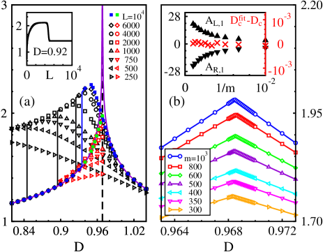
Figure 1: (color online) Entropy ${\cal S}$ as a function of $D$ for $J_{z}=1$. (a) Calculations with $m=1000$. Open symbols are obtained for the lowest energy level in Hilbert space $S^{\rm tot}_{z}=0$ with a range of $L$ values, solid symbols for $S^{\rm tot}_{z}=1$. Inset: $\ln 2$ drop in ${\cal S}(L)$ for $D=0.92$. (b) Bulk entropy ${\cal S}(D)$ close to the Gaussian critical point, computed with $L=10000$ for a range of $m$ values. Insets: fitting slopes $A_{L,1}$ and $A_{R,1}$ (left axis) and transition $D_{c}^{\rm fit}$ (right) obtained as functions of $m$.

Figure 1(a) contrasts the total and the bulk entropy. Calculations with small $L$ cannot access the unentangled regime, and for larger $L$ we find a $\ln 2$ jump when $D$ approaches $D_{c}$. For $L=10000$, the end-spins remain entangled for $0.94<D<D_{c}$. The maximum in the total entropy moves strongly with $L$, showing no direct indication of criticality rthcy . By contrast, in the Hilbert space $S^{\rm tot}_{z}=1$, the end-spins are unentangled in the lowest-energy state and this data reproduces exactly the bulk entropy. The location of the maximum in ${\cal S}$, shown in detail in Fig. 1(b), is clearly invariant with $m$. A linear fit to the bulk entropy on both sides of the transition in Fig. 1(b) gives our primary result, $D_{c}/J=0.96845$ with a minuscule error bar of 0.00008. The increasing slopes of the bulk entropy lines as $m\rightarrow\infty$ [inset Fig. 1(b)] indicate the onset of critical behavior.

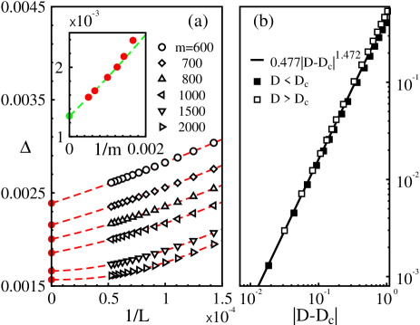
Figure 2: (color online) (a) Gap as a function of $L$, computed for $D/J=0.95$ with several values of $m$. Solid symbols for $L\rightarrow\infty$ are extrapolated to $m\rightarrow\infty$ (inset), giving $\Delta(0.95)=0.00130(4)$. (b) Extrapolated gaps as a function of $\left|D-D_{c}\right|$.

Having determined this extremely precise value of $D_{c}$, we may now discuss the critical behavior of the Gaussian transition with hitherto unattainable accuracy. We consider the physical quantities used in previous analyses of the transition rbjk ; rst ; rgjl ; rtnk ; rchs ; rdeor ; rthcy ; runk ; raho , beginning with the gap. To avoid effects in the gap extrapolation related to the disappearance of edge states, we use the lowest energy levels in the Hilbert spaces $S^{\rm tot}_{z}=1$ and $S_{z}^{\rm tot}=2$. Figure 2(a) illustrates our two-step extrapolation approach to compute the gap for the extremely numerically challenging point $D=0.95$, which lies very close to $D_{c}$. By following this procedure for all values of $D$, we show in Fig. 2(b) the approach of the gap to zero at $D_{c}$ from both the Haldane and large-$D$ sides. The closest four points, $D=0.925$, 0.95, 1.0, and 1.025, reveal a very narrow critical region, $|D-D_{c}|<0.1$, with critical exponent $\nu=1.472(4)$.

In a CFT for the Gaussian critical line cft , the gap $\Delta$ varies linearly and the energy $e_{g}$ quadratically with $1/L$. For the CFT analysis, we perform DMRG calculations with periodic BCs (PBCs) using $L=200$ and $m=2000$ [Figs. 3(a) and (b)]. We obtain the ground-state energy $e_{g}=-0.86856650(4)J$, velocity $v=2.564(2)J$, central charge $c\!=\!6\beta/\pi v\!=\!1.0006(8)$, Luttinger parameter $K\!=\!v/4\alpha\!=\!1.321(1)$, and critical exponent $\nu\!=\!1/(2\!-\!K)\!=\!1.472(2)$. This last agrees exactly with our gap data in Fig. 2(b), confirming the consistency and accuracy of our calculations. Our computed central charge is extraordinarily close to the expected value $c=1$ rchs ; rdeor . Even data at the extreme precision we attain cannot determine whether the second derivative of $e_{g}$ has a discontinuity [Fig. 3(c)], but set a very low upper bound. A continuous function with a point of inflection at $D_{c}$ is consistent with the CFT expectation rthcy that the Gaussian transition be third-order for $J_{z}=1$.

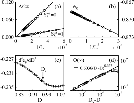
Figure 3: (color online) (a) Finite-size extrapolation of lowest two gaps at $D_{c}$. Fitting lines from CFT give $\Delta(S_{z}^{\rm tot}=0)=2\pi v/L$ with $v=2.564(2)J$ and $\Delta(S_{z}^{\rm tot}=1)=2\pi J\alpha/L$ with $\alpha=0.48516(1)$. (b) Extrapolated ground-state energy $e_{g}$ at $D_{c}$, with CFT fit $-0.86856650(4)J-\beta J/L^{2}$ and $\beta=1.3429(4)$. (c) Second derivative of extrapolated energy. (d) Extrapolated transverse string-order parameter (see text) of the Haldane phase, with fitting line $0.6036(4)|D-D_{c}|^{0.353(1)}$. Calculations for (a) and (b) performed with PBCs and $m=2000$, for (c) and (d) with OBCs and $m=1000$.

The transverse string-order parameter is defined as

$$O\left(l\right)=\left\langle\hat{S}^{x}_{0}\exp\left(i\pi\mbox{$\sum^{l-1}_{p=1}$}{\hat{S}}^{x}_{p}\right){\hat{S}}^{x}_{l}\right\rangle,$$ (3)

and encapsulates the incomplete $Z_{2}$$\times$$Z_{2}$ symmetry of the Haldane phase rls . To reduce the complexities inherent in calculating this quantity, we compute correlation functions only far from the system boundaries schollwock , in the left-central block $[L/4-1000,L/4]$ of the chain. We take the $S^{\rm tot}_{z}=1$ sector as the ground state. Figure 3(d) shows the results of our extrapolations to infinite $L$ and $m$. The string-order parameter clearly shows excellent scaling behavior in the critical regime. The scaling exponent $\nu^{\prime}=0.353(1)$ is very close to the value $1/\sqrt{8}$ predicted in the 2D classical model rls , demonstrating the common physics of the Gaussian, or preroughening, transition.

We illustrate with one example the utility of our improved DMRG calculations for investigating the entire Gaussian transition line. The point $J_{z}=0.5$ has been considered by several authors rchs ; rdeor ; rthcy ; runk . Our results (Fig. 4) provide the most accurate information yet available for this transition: $D_{c}/J=0.6355(6)$. The values of $L$ required to approach criticality are very much larger than for $J_{z}=1$ [Fig. 4(a)], and the accuracy is lower because ${\cal S}(D)$ is a significantly flatter function [Fig. 4(b)]. Our calculations with PBCs give $e_{g}=-0.91510889(1)J$, $v=2.185(2)J$, $c=1.000(1)$, $K=1.581(1)$, and $\nu=2.387(5)$ at $D_{c}$, allowing a complete characterization of the physics of continuously varying exponents.

We have considered the entropy ${\cal S}(m,L)$ at finite $m$ and $L$. In fact our results in Fig. 1 for $m=1000$ and $L=10000$ are fully converged for all values of $D$ outside the very narrow region $0.94<D<1.00$. We can deduce the critical behavior of ${\cal S}$ around $D_{c}$ from a massive quantum field theory rcc , in which ${\cal S}=(c/6)\ln\xi+A$ with $\xi=v/\Delta$ the correlation length and $\Delta\propto|D-D_{c}|^{\nu}$. The convergent behavior of our data near $D_{c}$ gives exactly the critical form ${\cal S}={\cal S}_{0}-(c\nu/6)\ln|D-D_{c}|$, which is shown as the solid lines diverging at $D_{c}$ in Figs. 1 and 4.

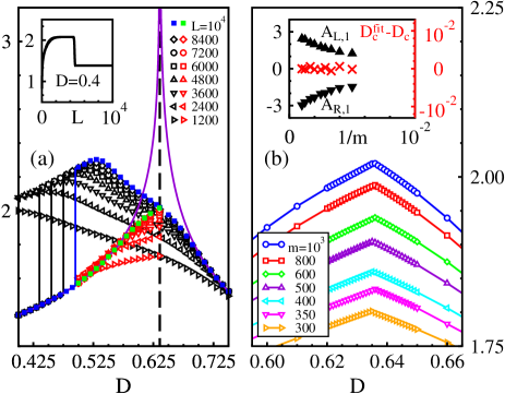
Figure 4: (color online) $S(D)$ as in Fig. 1 for $J_{z}=0.5$. (a) Values of $L$ as indicated. Inset: $\ln 2$ drop in ${\cal S}(L)$ for $D=0.4$. (b) Values of $m$ as indicated.

The Gaussian transition in the $S=1$ chain is topological, in that the parity of the ground state changes from negative in the Haldane phase to positive in the large-$D$ phase. The transition is thus associated with a change in the topological spin Berry phase from $\pi$ to 0 rtajn , and can be followed by a method of crossing energy levels (of states in the appropriate parity sectors). Our high-precision results demonstrate that this is indeed a very sensitive indicator of a topological transition: among all previous studies rbjk ; rst ; rgjl ; rtnk ; rchs ; rdeor ; rthcy ; runk ; raho , we find that the only accurate estimate of $D_{c}$ was obtained, despite being limited to 16-site systems, by employing this approach rchs .

We have demonstrated that the entropy is very valuable for discussing continuous phase transitions between gapped states. Many other types of strongly interacting quantum system fall in this category, one good example with electronic degrees of freedom being the ionic Hubbard model (IHM) rmmns . The numerically challenging transition in this case is of KT type. Continuous gapped-to-gapped transitions for both bosonic and fermionic systems exist in ultra-cold atomic condensates on optical lattices. The Gaussian transition has not yet been observed in experiment, due to difficulties in controlling the ratio $D/J$ in condensed matter systems, and cold-atom experiments may offer a clean solution to this problem.

To summarize, we calculate the critical point of the spin-one Heisenberg chain with single-ion anisotropy, $D_{c}/J=0.96845(8)$, to extremely high accuracy. To achieve this we introduce an improved DMRG scheme, which controls the absolute error of a large system and allows the elimination of end-spin effects. We exploit this accuracy to deduce the critical properties of many quantities at the Gaussian transition. The energy, entropy, and gap all show good scaling behavior with a single critical exponent, $\nu=1.472(2)$. We apply our technique also at $J_{z}=0.5$ to illustrate the continuous variability of exponents on the Gaussian transition line.

We thank A. A. Aligia and A. Honecker for helpful discussions. This work was supported by the National Science Foundation of China under Grant No. 10874244 and by Chinese National Basic Research Project No. 2007CB925001.

References

- (1)
- (2) A. Luther and D. J. Scalapino, Phys. Rev. B 16, 1153 (1977).
- (3) M. Den Nijs and K. Rommelse, Phys. Rev. B. 40, 4709 (1989).
- (4) F. D. M. Haldane, Bull. Am. Phys. Soc. 27, 181 (1982); Phys. Lett. 93A, 464 (1983); Phys. Rev. Lett. 50, 1153 (1983).
- (5) M. P. Nightingale and H. W. J. Blöte, Phys. Rev. B 33, 659 (1986).
- (6) S. R. White and R. M. Roack, Phys. Rev. Lett. 68, 3487 (1992); S. R. White, Phys. Rev. Lett. 69, 2863 (1992).
- (7) G. Xu el al., Phys. Rev. B. 54, 6827 (1996).
- (8) L. P. Regnault, I. Zaliznyak, J. P. Renard, and C. Vettier, Phys. Rev. B. 50, 9174 (1994).
- (9) A. Zheludev et al., Phys. Rev. B 53, 15004 (1996).
- (10) A. Zheludev et al., Phys. Rev. B 63, 104410 (2001).
- (11) H. J. Schulz, Phys. Rev. B 34, 6372 (1986).
- (12) R. Botet, R Jullien, and M. Kolb, Phys. Rev. B 28, 3914 (1983).
- (13) T. Sakai and M. Takahashi, Phys. Rev. B 42, 4537 (1990).
- (14) O. Golinelli, T. Jolicœur, and R. Lacaze, Phys. Rev. B 46, 10854 (1992).
- (15) T. Tonegawa, T. Nakao, and M. Kaburagi, J. Phys. Soc. Jpn. 65, 3317 (1996).
- (16) W. Chen, K. Hida, and B. C. Sanctuary, J. Phys. Soc. Jpn. 69, 237 (2000); erratum 77, 118001 (2008); Phys. Rev. B 67, 104401 (2003).
- (17) C. Degli Esposti Boschi, E. Ercolessi, F. Ortolani, and M. Roncaglia, Euro. Phys. J. B 35, 465 (2003).
- (18) Y. C. Tzeng and M. F. Yang, Phys. Rev. A 77, 012311 (2008); Y. C. Tzeng, H. H. Hung, Y. C. Chen, and M. F. Yang, Phys. Rev. A 77, 0623211 (2008).
- (19) H. Ueda, H. Nakano, and K. Kusakabe, Phys. Rev. B 78, 224402 (2008).
- (20) A. F. Albuquerque, C. J. Hamer, and J. Oitmaa, Phys. Rev. B 79, 054412 (2009).
- (21) H. W. J. Blöte, J. L. Cardy, and M. P. Nightingale, Phys. Rev. Lett. 56, 742 (1986).
- (22) P. Calabrese and J. Cardy, J. Stat. Mech. P06002 (2004).
- (23) M. Hagiwara et al., Phys. Rev. Lett. 65, 3181 (1990); S. H. Glarum et al., Phys. Rev. Lett. 67, 1614 (1991).
- (24) Ö. Legeza and J. Sólyom, Phys. Rev. Lett. 96, 116401 (2006); Ö. Legeza, J. Sólyom, L. Tincani, and R. M. Noack, Phys. Rev. Lett. 99, 087203 (2007).
- (25) U. Schollwöck, O. Golinelli, and T. Jolicœur, Phys. Rev. B 54, 4038 (1996).
- (26) See M. E. Torio, A. A. Aligia, G. I. Japaridze, and B. Normand, Phys. Rev. B 73, 115109 (2006).
- (27) S. R. Manmana, V. Meden, R. M. Noack, and K. Schönhammer, Phys. Rev. B 70, 155115 (2004).