Functionals of the Free Brownian Bridge

Abstract

We discuss the distributions of three functionals of the free Brownian bridge: its $\operatorname*{L}^{2}$-norm, the second component of its signature and its Lévy area. All of these are freely infinitely divisible. We introduce two representations of the free Brownian bridge as series of free semicircular random variables are used, analogous to the Fourier representations of the classical Brownian bridge due to Lévy and Kac.

1 Introduction

In this note we discuss the distributions of three non-commutative random variables defined in terms of a free Brownian bridge.

In his paper [11], Lévy introduces the following representation of the Brownian bridge. Let $\xi_{n},\eta_{n}$ be independent standard Gaussian random variables then the process defined by

$$\beta_{2\pi}(t) =\sum_{n=1}^{\infty}\frac{\cos(nt)-1}{n\sqrt{\pi}}\xi_{n}+\sum_{n=1}^{\infty}\frac{\sin(nt)}{n\sqrt{\pi}}\eta_{n}$$ (1.1)

defines a Brownian bridge on $$[0,2\pi] \eta_{n}$$. Another representation is given by Kac [9]. Retaining the notation for the it is a consequence of Mercer’s theorem that the Gaussian process defined by

$$\beta_{1}(t) =\sum_{n=1}^{\infty}\frac{\sin(nt)}{n\pi}\,\eta_{n}$$ (1.2)

has the covariance kernel of a Brownian bridge. The analogue of the Gaussian distribution and processes in non-commutative probability theory are the semicircle law and semicircular processes. It turns out that the crucial properties of the Gaussian distribution needed for the observations above are shared by the semicircular law. Therefore if we replace $\xi_{n},\eta_{n}$ by free standard semicirculars then (1.1) and (1.2) define free Brownian bridges on $[0,2\pi]$ and $[0,1]$ respectively. We will use this fact to prove various properties of the square norm, the second component of the signature and the Lévy area of the free Brownian bridge.

The $\operatorname*{L}^{2}$-norm of the classical Brownian bridge was first considered by Kac who used his representation (1.2) to compute its Fourier transform. Further calculations were performed using Kac’s work, see Tolmatz [17] and the references therein. We will compute the R-transform of the free analogue of this object and use the fact that its law is freely infinitely divisible to prove that it has a smooth density for which we give an implicit equation.

In [6] Capitaine and Donati-Martin construct the second component $Z$ of the signature of the free Brownian motion. This process plays a role in the theory of rough paths, see [6], Lyons[12] and Victoir[18] for details. The second component of the signature is a process taking values in the tensor product of the underlying non-commutative probability space with itself. Equipped with the product expectation this is a probability space in its own right and we compute the R-transform of $Z$. A connection between the cumulants of $Z$ and the number of 2-irreducible meanders, a combinatorial object introduced by Lando–Zwonkin[10] and further analysed by Di Francesco–Golinelli–Guitter [7] is pointed out.

Finally we apply the Lévy-type representation to compute the R-transform of the Lévy area corresponding to the free Brownian bridge. This random variable is also freely infinitely divisible. Once again this allows us to deduce that the law in question has a smooth density. Again we obtain an implicit equation.

From the considerations involving free infinite divisibility it also follows that the support of the law of both Lévy area and square norm is a single interval, in the former case symmetric about the origin, in the latter strictly contained in the positive half-line. In [15] a large deviations principle is established for the blocks of a uniformly random non-crossing partition. This result allows us to determine the maximum of the support from the free cumulants. We obtain implicit equations that determine the essential suprema of Lévy area and square norm.

Acknowledgements.

The author would like to thank his PhD advisor, Neil O’Connell for his advice and support in the preparation of this paper. We also thank Philippe Biane for helpful discussions and suggestions.

2 Free Probability Theory

We recall here some definitions and properties from free probability theory. For an introduction to the subject see for example [20, 19, 8].

2.1 Freeness, Distributions, and Transforms

Throughout let $(\mathcal{A},\phi)$ be a non-commutative probability space, i.e. a unital von Neumann algebra equipped with a state $\phi$ on $\mathcal{A}$. We think of elements $a\in\mathcal{A}$ as non-commutative random variables and consider $\phi(a)$ to be the expectation of $a\in\mathcal{A}$. We will only consider self-adjoint $a\in\mathcal{A}$. Then there exists a compactly supported measure $\mu_{a}$ on $\mathbb{R}$, called the distribution of $a$, such that

$$\phi(a^{n}) =\int t^{n}\,\mu_{a}(\mathrm{d}t)\quad\quad\forall\,n\in\mathbb{N}.$$

Recall that the Cauchy transform of $$\mu_{a}$$ is defined to be

$$G_{\mu_{a}}(z)=\int_{\mathbb{R}}\frac{\mu_{a}(\mathrm{d}t)}{t-z} =\sum_{n=0}^{\infty}\phi(a^{n})z^{-n-1}.$$

Since $\mu_{a}$ is compactly supported the first equality defines an analytic map $G_{\mu_{a}}\colon\mathbb{C}^{+}\longrightarrow\mathbb{C}^{-}$. The power series expansion is valid on a neighbourhood $U_{a}$ of infinity. We will also write $G_{a}$ for $G_{\mu_{a}}$.

Definition 2.1.

Von Neumann subalgebras $\mathcal{B}_{1},\ldots,\mathcal{B}_{N}$ of $\mathcal{A}$ are said to be free if for every set of indices $\{r_{j}\}_{j=1}^{m}\subseteq\{1,\ldots,N\}$ and collection $\{a_{j}\in\mathcal{B}_{r_{j}}\colon 1\leq j\leq m\}$ such that $r_{j}\neq r_{j+1}$ and $\phi(a_{j})=0\ \forall\,j\$ we already have

$$\phi(a_{1},\ldots,a_{m})=0.$$

Random variables $a_{1},\ldots,a_{N}$ are said to be free if the unital von Neumann algebras generated by the $a_{j}$ are free.

If $a$ and $b$ are free then the distribution of $a+b$ is uniquely determined by those of $a$ and $b$ (see Remark 2.5(2) below). Denote the laws of $a,b$ by $\mu_{1},\mu_{2}$ respectively. Then the free convolution of $\mu_{1}$ and $\mu_{2}$ is defined to be the distribution of $a+b$. Because self-adjoint elements of $\mathcal{A}$ are determined by their distribution this induces a binary operation on the space of compactly supported probability measures, denoted $\boxplus$.

A partition $\pi$ of the set $\underline{n}=\{1,\ldots,n\}$ is said to be crossing if there exist distinct blocks $V_{1}$, $V_{2}$ of $\pi$ and $x_{j},y_{j}\in V_{j}$ such that $x_{1}<x_{2}<y_{1}<y_{2}$. Otherwise $\pi$ is said to be non-crossing. Equivalently, arrange the numbers $1,\ldots,n$ clockwise on a circle and connect any two elements of the same block of $\pi$ by a straight line. Then $\pi$ is non-crossing if and only if the lines drawn are pairwise disjoint. Let $\operatorname*{NC}(n)$ denote the set of non-crossing partitions on $\underline{n}$.

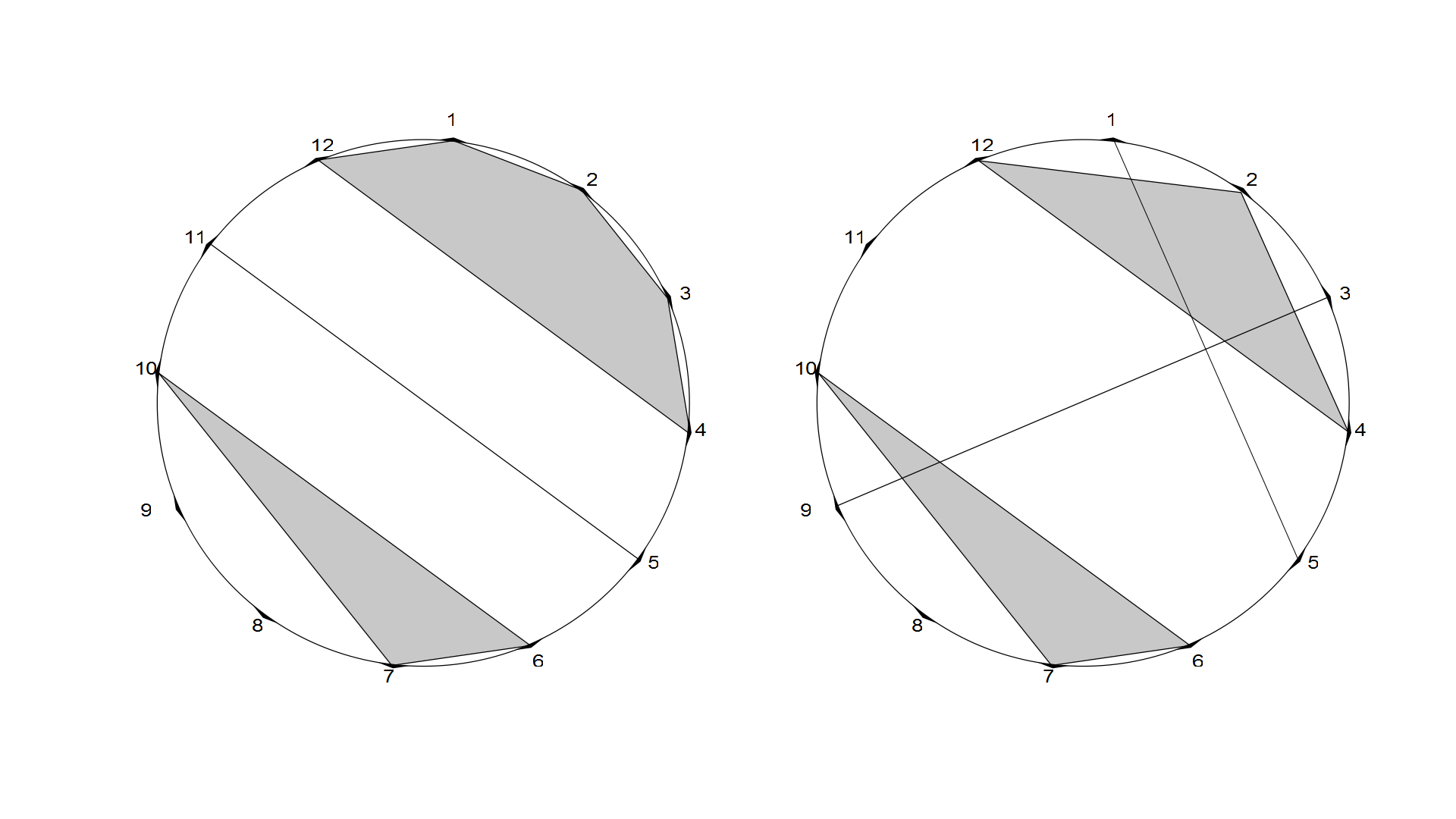
Figure 1: The partition $\{\{8\},\{9\},\{10,7,6\},\{11,5\},\{12,4,3,2,1\}\}$ is non-crossing, $\{\{5,1\},\{8\},\{9,3\},\{10,7,6\},\{12,4,2\}\}$ is crossing.

Definition 2.2.

The free cumulants of $\mathcal{A}$ are defined to be the maps $k_{n}\colon\mathcal{A}^{n}\longrightarrow\mathbb{C}$ ($n\in\mathbb{N}$) defined indirectly by the following system of equations:

$$\phi(a_{1},\ldots,a_{n}) =\sum_{\pi\in\text{NC}(n)}k_{\pi}[a_{1},\ldots,a_{n}]$$ (2.3)

where $$k_{\pi} \pi V_{1},\ldots,V_{r} \pi\in\operatorname*{NC}(n)$$ denotes the product of cumulants according to the block structure of . That is, if are the components of then

$$k_{\pi}[a_{1},\ldots,a_{n}] =k_{V_{1}}[a_{1},\ldots,a_{n}]\ldots k_{V_{n}}[a_{1},\ldots,a_{n}]$$

where, for $V=(v_{1},\ldots,v_{r})$ we just have $k_{V}[a_{1},\ldots,a_{n}]=k_{\left|V\right|}[a_{v_{1}},\ldots,a_{v_{r}}]$.

Note that (1.2) has the form $\phi(a_{1},\ldots,a_{n})=k_{n}[a_{1},\ldots,a_{n}]+$ lower order terms, so that we can find the $k_{n}$ inductively. Alternatively, (2.3) defines the $k_{n}$ by Möbius inversion. See [14] for details.

We will write $k_{n}(a)$ for $k_{n}[a,\ldots,a]$. The R-transform of a random variable $a\in\mathcal{A}$ is defined to be the formal power series

$$R_{a}(z) =\sum_{n=0}^{\infty}k_{n+1}(a)z^{n}.$$ (2.4)

If the law of $$a G_{a} a K_{a}$$ has compact support then equation (2.4) defines an analytic function on a neighbourhood of zero [8, Theorem 3.2.1]. Moreover the Cauchy transform of is locally invertible on a neighbourhood of infinity and the inverse satisfies

$$K_{a}(z) =R_{a}(z)+\frac{1}{z}.$$

Remark 2.5.

The following three properties of the R-transform are easy to check using the continuity of $\phi$ and multilinearity of the cumulants.

1. If $a_{n}\longrightarrow a\in\mathcal{A}$ then $R_{a_{n}}(z)\longrightarrow R_{a}(z)$ as $n\to\infty$

2. If $a,b\in\mathcal{A}$ are free then $R_{a+b}(z)=R_{a}(z)+R_{b}(z)$

3. For $\lambda\in\mathbb{C}$ we have $R_{\lambda a}(z)=\lambda R_{a}(\lambda z)$.

2.2 Semicircular Processes

Definition 2.6.

A collection $\mathcal{S}=(s_{j})_{j\in I}$ of non-commutative variables on $\mathcal{A}$ is said to be a semicular family with covariance $\left(c(i,j)\right)_{i,j\in I}$ if the cumulants are given by

$$k_{\pi}[s_{j_{1}},\ldots s_{j_{n}}] =\prod_{p\sim_{\pi}q}c(j_{p},j_{q}).$$

If $\mathcal{S}$ consists of a singleton $s_{1}$ and $r=2\sqrt{c(1,1)}$ then the distribution of $s_{1}$ is the centred semicircle law of radius $r$, that is the measure $\sigma_{r}$ on $\mathbb{R}$ given by

$$\sigma_{r}(\mathrm{d}t) =\frac{2}{\pi r^{2}}\sqrt{r^{2}-t^{2}}\ \mathbf{1}_{[-r,r]}(t)\,\mathrm{d}t.$$

In particular $\sigma_{2}$ is also called the standard semicircle law and non-commutative random variables with law $\sigma_{r}$ ($\sigma_{2}$) are referred to as (standard) semicirculars.

The semicircle law plays a similar role to the Gaussian distribution on classical probability theory. In particular there exists a central limit theorem [20, Theorem 3.5.1], and a collection of random variables with a joint semicircular law is determined by its covariance. To be more precise we recall the following

Proposition 2.7 (Nica–Speicher[14], Proposition 8.19).

Let $(s_{i})_{i\in I}$ be a semicircular family of covariance $(c(i,j))_{i,j\in I}$ and suppose $I$ is partitioned by $I_{1},\ldots,I_{d}$. Then the following are equivalent:

1. The collections $\{s_{j}\colon j\in I_{1}\},\ldots,\{s_{j}\colon j\in I_{d}\}$ are free

2. We have $c(r,j)=0$ whenever $r\in I_{p}$ and $j\in I_{q}$ with $p\neq q$.

In particular $\{s_{j}\colon j\in I\}$ is a free family if and only if $C=(c(r,j))_{r,j\in I}$ is diagonal.

Definition 2.8.

A process $(X(t))_{t\geq 0}$ on $\mathcal{A}$ is said to be a semicircular process if for every $t_{1},\ldots,t_{n}\in[0,\infty)$, the set $\left(X(t_{1}),\dots,X(t_{n})\right)$ is a semircular family.

By the considerations above the finite-dimensional distributions of a semicircular process are determined by the covariance structure of the process, i.e. by the function $C\colon[0,\infty)^{2}\longrightarrow\mathbb{C}$ defined by

$$C(s,t) =\phi(X(s)X(t)).$$

.

2.3 The Lévy Representation of the Free Brownian Bridge

Definition 2.9.

A centred semicircular process $\left(\beta_{T}(t)\right)_{t\in[0,T]}$ on $\mathcal{A}$ is said to be a free Brownian bridge on $[0,T]$ if its covariance structure is given by

$$\phi(\beta_{T}(s)\beta_{T}(t))=s\wedge t-\frac{st}{T}.$$

Remark 2.10.

In analogy with classical probability it can be easily checked that if $\beta$ is a free Brownian bridge on $[0,1]$ and $\xi_{0}$ is a free standard semicircular free from $\{\beta(t)\colon t\in[0,1]\}$, then $X(t)=\xi_{0}t+\beta(t)$ defines a free Brownian motion, that is

1. the distribution of $X(t)$ is a centred semicircular law with radius $t$;

2. $X(t)-X(s)$ is free from $\{X(r)\colon r\leq s\}$

3. $X(t)-X(s)$ has the same distribution as $X(t-s)$.

The following proposition is the analogue of Lévy’s representation of the classical Brownian bridge [11]. Its proof follows from the fact that centred semicircular processes are determined by their covariance and that (non-commutative) covariances of the $\xi_{n},\eta_{n}$ are the same as the (commutative) covariances of a corresponding independent family of standard Gaussian variables.

Proposition 2.11.

Let $\{\xi_{n},\eta_{m}\colon(n,m)\in\mathbb{N}_{0}\times\mathbb{N}\}$ be a set of free standard semicircular variables in $\mathcal{A}$. Then the process $\beta_{2\pi}$ defined by

$$\beta_{2\pi}(t) =\sum_{n=1}^{\infty}\frac{\cos(nt)-1}{n\sqrt{\pi}}\xi_{n}+\sum_{n=1}^{\infty}\frac{\sin(nt)}{n\sqrt{\pi}}\eta_{n}$$ (2.12)

is a free Brownian bridge on $[0,2\pi]$.

2.4 A Representation for Centred Semicircular Processes

In this section we show how Kac’s representation[9] for the classical Brownian bridge on the unit interval can be translated into the setting of free probability. His method extends to all centred semicircular (or indeed Gaussian) processes, as follows. Everything relies on the following classical result from functional analysis, see Bollobas [5].

Theorem 2.13 (Mercer’s theorem).

Let $K\colon[a,b]\times[a,b]\longrightarrow\mathbb{R}$ be a non-negative definite symmetric kernel. Denote by $\mathcal{H}$ the Hilbert space $\operatorname*{L}^{2}[a,b]$ and let $T_{K}$ be the operator on $\mathcal{H}$ associated to $K$, that is,

$$T_{K}(f)(s) =\int_{a}^{b}K(s,t)\,f(t)\ \mathrm{d}t.$$ (2.14)

Then there exists an orthonormal basis $$(f_{n})_{n\in\mathbb{N}} \mathcal{H} T_{K} \lambda_{n} f_{n}\in\mathcal{C}[a,b] \lambda_{n}\neq 0$$ of  consisting of eigenfunctions of such that the corresponding eigenvalues are non-negative, whenever and

$$K(s,t) =\sum_{n=1}^{\infty}\lambda_{n}f_{n}(s)f_{n}(t)$$ (2.15)

where the convergence is absolute and uniform, and hence also in $\operatorname*{L}^{2}[a,b]$.

We can use Mercer’s theorem to represent any centred semicircular process as a series of free standard semicircular random variables, noting that if $Y$ is a centred semicircular process on $[a,b]$ then its covariance function $K$ defined by $K(s,t)=\phi(Y(s)Y(t))$ is a non-negative symmetric kernel on $[a,b]$.

Corollary 2.16.

Let $K,\mathcal{H},(\lambda_{n},f_{n})_{n\in\mathbb{N}}$ be as in Mercer’s theorem and let $(\eta_{n})_{n\in\mathbb{N}}$ be a sequence of free standard semicirculars. Then the process $Y$ defined by

$$Y(t) =\sum_{n=1}^{\infty}\sqrt{\lambda_{n}}f_{n}(t)\,\eta_{n}$$ (2.17)

is a centred semicircular process of covariance $K$.

Proof.

It is immediate that $Y$ is a centred semircircular process. Its covariance kernel is given by

$$\phi(Y(s)Y(t)) =\sum_{m,n=1}^{\infty}\sqrt{\lambda_{m}\lambda_{n}}f_{m}(s)f_{n}(t)\phi(\eta_{m}\eta_{n})$$

$$=\sum_{n=1}^{\infty}\lambda_{n}f_{n}(s)f_{n}(t)=K(s,t)$$

by Mercer’s theorem. ∎

For the free Brownian bridge on $[0,1]$ we have $K(s,t)=s\wedge t-st$. Solving the corresponding eigenvalue-eigenvector equation we obtain Kac’s representation in the free setting:

$$\beta_{1}(t) =\sum_{n=1}^{\infty}\frac{\sin(nt)}{n\pi}\,\eta_{n}.$$ (2.18)

3 Square Norm of the Free Brownian Bridge

In this section we consider the square-norm of a free Brownian bridge $\beta$ on interval. Recall that $\mathcal{A}$ is a von Neumann algebra so that we can consider $\beta$ as a map from $[0,1]$ into a Banach space which is easily seen to be continuous. We can therefore use Riemann integration to define

$$\Gamma =\int_{0}^{1}\beta(t)^{2}\,\mathrm{d}t$$

where $$\beta [0,1] \Gamma \Gamma$$ is a free Brownian bridge on . In this section we discuss the distribution of the non-commutative random variable , using the representation (2.18). Kac[9] showed that the Laplace transform of the commutative analogue of is given by

$$\widehat{f}(p) =\left(\frac{\sqrt{2p}}{\sinh{\sqrt{2p}}}\right)^{(1/2)}.$$

Other properties, in particular the density function $f$, were computed, most recently by Tolmatz[17].

We give here the R-transform of $\Gamma$ and an expression for its moments involving a sum over non-crossing partitions. Further below we show that the distribution $\mu_{\Gamma}$ of $\Gamma$ is freely infinitely divisible. This gives us some analytic tools to show that there exist $a,b\in\mathbb{R}$ with $0<a<b<1$ such that the support of $\mu_{\Gamma}$ is $[a,b]$ and that $\mu_{\Gamma}$ has a smooth positive density on $[a,b]$. We give an implicit equation and a sketch for the density.

Finally we use a result from [15] to characterise the maximum $b$ of the support of $\mu_{\Gamma}$.

3.1 The R-transform

Proposition 3.1.

The R-transform of $\Gamma$ is given by

$$R_{\Gamma}(z) =\frac{1-\sqrt{z}\cot(\sqrt{z})}{2z}.$$ (3.2)

Proof.

By orthonormality of the functions $\sin(nt)$ we have

$$\Gamma =\frac{1}{\pi^{2}}\,\sum_{n=1}^{\infty}\frac{1}{n^{2}}\eta_{n}^{2}.$$ (3.3)

The square of a standard semicircular random variable is a free Poisson element of unit rate and jump size (Nica–Speicher[14], Proposition 12.13). So the Cauchy transform of $\eta_{n}$ is given by [14]

$$G_{n}(z)=\sum_{n=0}^{\infty}c_{m}z^{-m-1} =\frac{1}{z}C\left(\frac{1}{z}\right)=\frac{1}{2}+\sqrt{\frac{1}{4}-\frac{1}{z}}.$$

The free cumulants of $$\eta_{n}^{2}$$ are all equal to 1 and the R-transform is given by

$$R_{n}(z) =\frac{1}{1-z},\quad\quad\left|z\right|<1.$$

Using the properties of the R-transform mentioned in Remark 2.5) we obtain for $\left|z\right|<\pi^{2}$

$$R_{\Gamma}(z) =\sum_{n=1}^{\infty}\frac{1}{\pi^{2}n^{2}}R_{n}\left(\frac{z}{\pi^{2}n^{2}}\right)=\sum_{n=1}^{\infty}\frac{1}{n^{2}\pi^{2}-z}=\frac{1-\sqrt{z}\cot(\sqrt{z})}{2z}$$

as claimed. ∎

The free cumulants of $\Gamma$ are therefore given by

$$k_{m} =\frac{\zeta(2m)}{\pi^{2m}}=(-4)^{m}\,\frac{B_{2m}}{(2m)!}$$

where $$B_{n} n^{\text{th}} \zeta$$ is the Bernoulli number and the Riemann zeta function. With (2.3) we obtain a formula for the moments involving a sum over non-crossing partitions:

$$\phi\left(\Gamma^{n}\right) =\ \frac{1}{\pi^{2n}}\sum_{\sigma\in\operatorname*{NC}(n)}\prod_{r=1}^{m_{\sigma}}\zeta(2l_{r}^{\sigma})=(-4)^{n}\sum_{\sigma\in\operatorname*{NC}(n)}\prod_{r=1}^{m_{\sigma}}\frac{B_{2l_{r}^{\sigma}}}{(2l_{r}^{\sigma})!}$$

where $m_{\pi}$ denotes the number of equivalence classes of $\pi$ and $l_{r}^{\pi}$ is the size of the $r^{\text{th}}$ equivalence class of $\pi$.

While there does not seem to exist a closed-form expression for the inverse of $K_{\Gamma}(z)=R_{\Gamma}(z)-\frac{1}{z}$ (and hence, by the Stieltjes inversion formula, for the density) we will describe some properties of the law $\mu_{\Gamma}$ of $\Gamma$. We will prove that $\mu_{\Gamma}$ is freely infinitely divisible, has a positive analytic density on a single interval and give an equation for the right end point of that interval.

3.2 Free Infinite Divisibility

The concept of infinite divisibility has a natural analogue in free probability theory. Noting that the square norm of the free Brownian bridge is freely infinitely divisible we will use the approach of P. Biane in his appendix to the paper [2] to prove that the law of $\Gamma$ has a smooth density on its support and give an implicit formula for that density.

Definition 3.4.

A compactly supported probability measure $\mu$ is said to be freely infinitely divisible (or $\boxplus$-infinitely divisible) if for every $n\in\mathbb{N}$ there exists a compactly probability measure $\mu_{n}$ such that

$$\mu =\mu_{n}^{\boxplus n}=\underbrace{\mu_{n}\boxplus\ldots\boxplus\mu_{n}}_{n\text{ times}}$$

where $\boxplus$ denotes free convolution (Section 2).

Since each $\xi_{n}$ has a free Poisson distribution and is therefore freely infinitely divisible it follows that $\Gamma$ is also $\boxplus$-infinitely divisible.

Recall that the Cauchy transform $G_{\Gamma}$ of $\Gamma$ is an analytic map from the upper half plane $\mathbb{C}^{+}$ into the lower half plane $\mathbb{C}^{-}$, which is locally invertible on a neighbourhood of infinity, and that its local inverse is given by the K-transform $K_{\Gamma}$ where

$$K_{\Gamma}(z) =R_{\Gamma}(z)+\frac{1}{z}=\frac{3-\sqrt{z}\cot\left(\sqrt{z}\right)}{2z}.$$

From Proposition 5.12 in Bercovici–Voiculescu [3] and the infinite divisibility of $\Gamma$ it is straightforward to deduce the following result.

Lemma 3.5.

The law $\mu_{\Gamma}$ of the square norm of the free Brownian bridge can have at most one atom. Moreover its Cauchy transform $G_{\Gamma}$ is an analytic injection from $\mathbb{C}^{+}$ whose image is the connected component $\Omega$ in $\mathbb{C}^{-}$ of

$$\widehat{\Omega} =\{z\in\mathbb{C}^{-}\colon\mathfrak{Im}\left(K_{\Gamma}(z)\right)>0\}$$

that contains $iy$ for small values of $y$.

It will be useful to characterise the boundary $\partial\Omega$.

Lemma 3.6.

For every $t\in(\pi,2\pi)$ there exists unique $r(t)>0$ such that $\mathfrak{Im}\left[\left(K_{\Gamma}(r(t)e^{it})\right)\right]=0$. Moreover

$$\left.\frac{\partial}{\partial z}\mathfrak{Im}K_{\Gamma}(z)\right|_{z=r(t)e^{it}} \neq 0\quad\quad\qquad\forall\,t\in(\pi,2\pi).$$ (3.7)

Proof.

Fix $t\in(\pi,2\pi)$. The imaginary part of $K_{\Gamma}$ can be written in polar co-ordinates by

$$h_{t}(r):=K_{\Gamma}\left(r\,e^{it}\right) =-\frac{3\sin(t)}{2r}+\frac{\gamma\sinh(\sigma\sqrt{r})\cosh(\sigma\sqrt{r})+\sigma\sin(\gamma\sqrt{r})\cos(\gamma\sqrt{r})}{2\sqrt{r}\left(\sin^{2}(\gamma\sqrt{r})+\sinh^{2}(\sigma\sqrt{r})\right)}$$

where $$\sigma=\sin(t/2) \gamma=\cos(t/2) g_{t}(r)=2r\,h_{t}(r^{2})$$ and . Define . Then

$$g_{t}(r) =-\frac{6\sigma\gamma}{r}+\frac{\sigma\sin\left(2\gamma r\right)+\gamma\sinh\left(2\sigma r\right)}{2\left[\sin^{2}(\gamma\sqrt{r})+\sinh^{2}(\sigma\sqrt{r})\right]}.$$

It is a lengthy but simple calculation to prove the existence of unique $\rho(t)>0$ such that $g_{t}(\rho(t))=0$ and that $g_{t}^{\prime}(\rho(t))<0$. The result follows. ∎

Therefore $\widehat{\Omega}$ is actually simply connected: it is given by the area enclosed by the real axis and the curve $\lambda=\{r_{t}e^{it}\colon t\in(\pi,2\pi)\}$. In particular $\Omega=\widehat{\Omega}$ and $\partial\Omega$ is a continuous simple curve. So Carathéodory’s theorem applies, wherefore the analytic bijection $G_{\Gamma}\colon\mathbb{C}^{+}\longrightarrow\Omega$ extends to a homeomorphism (denoted $\widehat{G}_{\Gamma}$) from $\mathbb{C}^{+}\cup\mathbb{R}\cup\{\infty\}$ to the closure $\overline{\Omega}$ of $\Omega$ in $\mathbb{C}\cup\{\infty\}$.

Since $\Omega$ is bounded, so is its closure, whence $\widehat{G}_{\Gamma}$ is finite on $\mathbb{C}^{+}\cup\mathbb{R}\cup\{\infty\}$. The set of isolated points of the support of $\mu_{\Gamma}$ is exactly the set of $t\in\mathbb{R}$ such that $\widehat{G}_{\Gamma}(t)=\infty$ so $\operatorname*{supp}(\mu_{\Gamma})$ must be an interval $[a,b]$. From the Stieltjes inversion formula (see for example [8], p.93) it now follows that if we put for $x\in[a,b]$

$$\Phi(x) =-\frac{1}{\pi}\lim_{y\to 0}\mathfrak{Im}\left(G_{\Gamma}(x+iy)\right)=-\frac{1}{\pi}\,\mathfrak{Im}\left(\widehat{G}_{\Gamma}(x)\right)$$ (3.8)

then $\mu_{\Gamma}$ has density $\Phi$ with respect to Lebesgue measure on $[a,b]$. Since $K_{\Gamma}$ is the inverse of $G_{\Gamma}$ and because of (3.7) the implicit function theorem applies and hence $\Phi$ is smooth on $[a,b]$. Moreover it follows that

$$\operatorname*{supp}\mu_{\Gamma} =K_{\Gamma}\left(\partial\Omega\cap\mathbb{C}^{-}\right)=\left[K_{\Gamma}\left(r_{\pi+}\right)\wedge K_{\Gamma}\left(r_{2\pi-}\right),K_{\Gamma}\left(r_{\pi+}\right)\vee K_{\Gamma}\left(r_{2\pi-}\right)\right].$$

where $r_{\pi+}=\lim_{s\downarrow 0}r_{\pi+s}$ and $r_{2\pi-}=\lim_{s\downarrow 0}r_{2\pi-s}$.

The operator $\Gamma$ is positive and its norm is less than 1, so the support of $\mu_{\Gamma}$ must be contained in the unit interval. We summarise the results of this section.

Proposition 3.9.

There exist $a,b\in\mathbb{R}$ such that $0\leq a<b\leq 1$ and a positive smooth function $\Phi\colon[a,b]\longrightarrow\mathbb{R}$ such that

$$\mu_{\Gamma}(\mathrm{d}t) =\Phi(t)\mathbf{1}_{[a,b]}(t).$$ (3.10)

The function $\Phi$ is given by $\Phi(x)=-\frac{1}{\pi}r(t_{x})\sin(\tau_{x})$ where $\tau_{x}\in(\pi,2\pi)$ is the unique solution to $K_{\Gamma}\left(r(\tau_{x})\,e^{i\tau_{x}}\right)=x$.

Below is a sketch of the density function based on numerical computations.

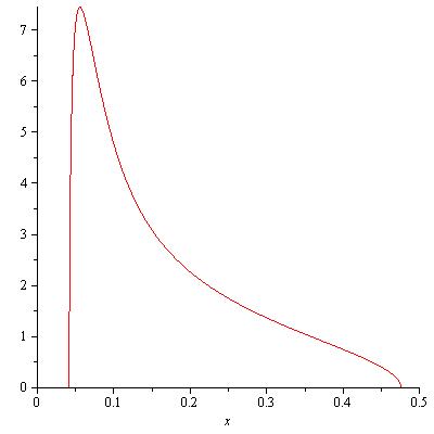
Figure 2: Density of the $\operatorname*{L}^{2}$-norm of the free Brownian bridge.

3.3 The Maximum of the Support

We now study the maximum of the support of $\mu_{\Gamma}$. We will need Theorem 5.4 from [15]:

Theorem 3.11.

Let $\mu$ be a compactly supported probability measure on $[0,\infty)$ such that its free cumulants $(k_{j})_{j\in\mathbb{N}}$ are all positive. Then the right edge $\rho_{\mu}$ of the support of $\mu$ is given by

$$\log\rho_{\mu} =\sup\left\{\frac{1}{m_{1}(p)}\sum_{m=1}^{\infty}p_{m}\log\left(\frac{k_{m}}{p_{m}}\right)+\frac{\Theta\big{(}m_{1}(p)\big{)}}{m_{1}(p)}\colon p\in\mathfrak{M}_{1}^{1}(\mathbb{N})\right\}$$ (3.12)

where $\mathfrak{M}_{1}^{1}(\mathbb{N})=\{p\in\mathfrak{M}_{1}(\mathbb{N})\colon m_{1}(p)<\infty\}$ is the set of probability measures on $\mathbb{N}$ with finite mean and $\Theta(m)=\log(m-1)-m\log\left(1-\frac{1}{m}\right)$.

It turns out that this variational problem can be solved using the method of Laplace multipliers. There exists a unique maximiser $p^{*}$ for the supremum on the right-hand side of (3.12). Using the series expansion of $\zeta(2n)$ and interchanging summation we obtain

$$p^{*}_{n} =\frac{1}{m^{*}-1}\,\zeta(2n)\left(\frac{\gamma}{\pi}\right)^{2n}$$

where $$\gamma m^{*} m^{*} \left(\frac{2}{3},\infty\right)$$ is a rational function of and is the unique solution on of the equation

$$m-3 =\sqrt{4m^{2}-2m-6}\,\cot\left(\frac{4m^{2}-2m-6}{m-1}\right)$$ (3.13)

In the end we obtain an implicit equation for the right edge of the support of $\mu_{\Gamma}$:

Proposition 3.14.

The number $b$ from Proposition 3.9 is given by

$$b=\frac{\left(m^{*}\right)^{2}-m^{*}}{4\left(m^{*}\right)^{2}-2m^{*}-6}$$

where $m^{*}$ is the unique solution of $(\ref{Eq:MStarSquare})$ on $\left(\frac{2}{3},\infty\right)$.

4 The Signature of the Free Brownian Bridge

4.1 Signature and Rough Paths

In T. Lyons’s paper [12] a new approach to differential equations driven by rough paths is proposed. For a general Banach-valued path $p\colon\mathbb{R}_{+}\longrightarrow E$ we define, when this makes sense, the signature of $p$ to be the process $S(p)$ taking values in the tensor algebra $T((E))=\bigoplus_{n=0}^{\infty}E^{\otimes n}$ whose $n^{\text{th}}$ component is given by the $n$-times iterated integral against $p$:

$$S(p)_{n}(t) =\int_{0<t_{1}<\ldots<t_{n}<t}\mathrm{d}p\,(t_{1})\otimes\ldots\otimes\mathrm{d}p\,(t_{n}).$$

The signature is then used to solve general differential equations of the form

$$\mathrm{d}\,S(t) =S(t)\otimes\mathrm{d}p\,(t).$$

In order to show that this works if the path in question is a free Brownian motion $X$, Capitaine–Donati-Martin[6] define an integral of a class of suitable processes $\mathfrak{P}$ against $X$ that yields a process taking values in the tensor product $\mathcal{A}\otimes\mathcal{A}$ and prove that $X$ itself is contained in $\mathfrak{P}$. The integral is defined taking Riemann-type approximations, so it is straightforward to extend it to processes with finite variation. Using Remark 2.10 we can therefore define the second component of the signature of a free Brownian bridge $\beta$ on $[0,2\pi]$ by

$$Z(t) =\int_{0}^{t}\beta\otimes\mathrm{d}\,\beta\quad\quad t\in[0,2\pi]$$

where the integral is in the sense of [6], see also Victoir[18].

If $\mathcal{A}$ is a von Neumann algebra and $\phi$ a faithful tracial state on $\mathcal{A}$ then its tensor product $\phi\otimes\phi$ is a faithful tracial state on the von Neumann tensor product $\mathcal{A}\otimes\mathcal{A}$ of $\mathcal{A}$ with itself, see for example [18], p. 109. So we can consider $(\mathcal{A}\otimes\mathcal{A},\phi\otimes\phi)$ as a non-commutative probability space in its own right. We will discuss here the law of $Z(2\pi)$ with respect to this space.

We will also use the notation $\widehat{\mathcal{A}},\ \widehat{\phi}$ for $\mathcal{A}\otimes\mathcal{A}$, $\phi\otimes\phi$ respectively.

4.2 Using the Lévy Representation

The representation (2.12) and a straightforward calculation using orthogonality of the trigonometric functions yield

Proposition 4.1.

The Lévy area of the free Brownian bridge at time $2\pi$ is the random variable

$$Z(2\pi) =\sum_{n=1}^{\infty}\frac{1}{n}\left(\xi_{n}\otimes\eta_{n}-\eta_{n}\otimes\xi_{n}\right).$$ (4.2)

In order to further analyse this series we need to know how the $\xi_{m}\otimes\eta_{m}$, $\eta_{m}\otimes\xi_{m}$ are correlated. The following technical lemma is in a slightly more general framework than we need here.

Lemma 4.3.

Let $\{a_{n},b_{n}\colon n\in\mathbb{N}\}$ be a collection of free random variables in $\mathcal{A}$ such that for each $n$ the variables $a_{n},b_{n}$ are identically distributed. Then the following set is free in $\mathcal{A}\otimes\mathcal{A}$:

$$\{a_{n}\otimes b_{n},b_{m}\otimes a_{m}\colon m,n\in\mathbb{N}\}.$$

Proof.

Let $X_{k}\in A(\mathbf{1},\alpha_{j_{k}}\otimes\beta_{j_{k}})$ such that $j_{k}\neq j_{k+1}$ for $k\in\{1,\ldots,m-1\}$ and for each $k$ we have $\{\alpha_{k},\beta_{k}\}=\{a_{j_{k}},b_{j_{k}}\}$. Suppose moreover that each $\widehat{\phi}(X_{k})=0$. We need to show that $\widehat{\phi}(X_{1}\ldots X_{m})=0$. Note that $X_{k}=p_{k}(\alpha_{k}\otimes\beta_{k})$ for some polynomial $p_{k}$. Since addition and multiplication in the tensor product act componentwise

$$\widehat{\phi}(X_{1}\ldots X_{m}) =\widehat{\phi}\left((p_{1}(\alpha_{j_{1}})\otimes p_{1}(\beta_{j_{1}}))\ldots(p_{m}(\alpha_{j_{m}})\otimes p_{m}(\beta_{j_{m}}))\right)$$

$$=\widehat{\phi}\left[(p_{1}(\alpha_{j_{1}})\ldots p_{m}(\alpha_{j_{m}}))\otimes(p_{1}(\beta_{j_{1}})\ldots p_{m}(\beta_{j_{m}}))\right]$$

$$=\phi\left(p_{1}(\alpha_{j_{1}})\ldots p_{m}(\alpha_{j_{m}})\right)\ \phi\left(p_{1}(\beta_{j_{1}})\ldots p_{m}(\beta_{j_{m}})\right).$$

By freeness of the $a_{n},b_{n}$ and the fact that $j_{k}\neq j_{k+1}$ each of $\alpha_{j_{1}},\ldots,\alpha_{j_{m}}$ and $\beta_{j_{1}},\ldots\beta_{j_{m}}$ are free. Since $\widehat{\phi}(X_{k})=0$ we have $\phi(p_{k}(\alpha_{j_{k}}))\phi(p_{k}(\beta_{j_{k}}))=0$. So one of the factors must vanish. But since $\alpha_{j_{k}},\beta_{j_{k}}$ are identically distributed, either both or none of them are zero. So $\phi(p_{k}(\alpha_{j_{k}}))=\phi(p_{k}(\beta_{j_{k}}))=0$ for all $k$. Freeness now implies that the last line, and hence $\widehat{\phi}(X_{1}\ldots X_{m})=0$, vanishes. ∎

So the set $\{\xi_{n}\otimes\eta_{n},\eta_{n}\otimes\xi_{n}\colon n\in\mathbb{N}\}$, and hence the terms of the right hand side of (4.2), are free. Since the R-transform is additive on free random variables we will use this tool to compute the distribution of $Z(2\pi)$ in $(\widehat{\mathcal{A}},\widehat{\phi})$. From Lemma 4.3 we can deduce

Corollary 4.4.

The R-transform of $Z(2\pi)$ is given by

$$R_{Z(2\pi)}(z) =2\,\sum_{n=1}^{\infty}\frac{1}{n}\,R_{\xi\otimes\eta}\left(\frac{z}{n}\right).$$ (4.5)

Remark 4.6.

By the definition of $\widehat{\phi}$ we have $\widehat{\phi}\left((\xi\otimes\eta)^{k}\right)=\phi(\xi^{k})^{2}$ for $k\in\mathbb{N}$. Recall that $R_{a}(z)=\sum_{m=1}^{\infty}k_{m+1}(a)z^{m}$ where $k_{m}(a)$ denotes the $m^{\text{th}}$ cumulant of $a$. In particular $k_{1}(\xi\otimes\eta)=\phi(\xi)^{2}=0$ so that (on a neighbourhood of zero) $R_{\xi\otimes\eta}(z)=zP(z)$ for some $P\in\mathbb{C}[z]$. Rewriting (4.5) yields

$$R_{Z(2\pi)}(z) =2\,\sum_{n=1}^{\infty}\frac{1}{n^{2}}\,P\left(\frac{z}{n}\right),$$ (4.7)

in particular the right hand side of (4.5) converges in a neighbourhood of zero.

4.3 The Distribution of $\xi\otimes\eta$ and Meanders

We proceed to compute the R-transform of $\zeta:=\xi\otimes\eta$ with $\xi,\eta$ free standard semicirculars. Recall that the odd moments of $\xi$ vanish and that $\phi(\xi^{2n})$ is given by the $n^{\text{th}}$ Catalan number

$$\phi(\xi^{2n}) =C_{n}:=\frac{1}{2n+1}\begin{pmatrix}2n\\ n\end{pmatrix}.$$ (4.8)

Since $$\xi \eta \zeta \nu \mathbb{R} \nu$$, are self-adjoint, so is . Hence its law is a probability measure with compact support in . In particular is determined by its moments which are given by

$$\int t^{m}\nu(\mathrm{d}t)=\phi\left((\xi\otimes\eta)^{m}\right) =\phi(\xi^{m})\phi(\eta^{m})=\begin{cases}\left(C_{k}\right)^{2}\quad&\text{if }m=2k\\ 0&\text{ if }m\text{ is odd}\end{cases}$$ (4.9)

i.e. $\nu$ is the law of $\zeta_{1}\zeta_{2}$ where the $\zeta_{i}$ are independent commutative random variables with standard semicircular distribution. Therefore $\nu$ is absolutely continuous with respect to Lebesgue measure with density $\phi$ given by

$$\phi(t) =\frac{1}{4\pi^{2}}\int_{-\left|t\right|/2}^{\left|t\right|/2}\sqrt{4-x^{2}}\,\sqrt{4x^{2}-t^{2}}\,\mathrm{d}x\ \ 1_{[-2,2]}(t).$$ (4.10)

The Catalan numbers $C_{n}$ are well-known in combinatorics. They give, for example, the number of Dyck paths of length $2n$. Similarly there is a combinatorial interpretation of the squares of the Catalan numbers, as detailed in Lando–Zwonkin[10] and Di Francesco–Golinelli–Guitter[7]: consider an infinite line in the plane and call it the river. A meander of order $n$ is a closed self-avoiding connected loop intersecting the line through $2n$ points (the bridges). Two meanders are said to be equivalent if they can be deformed into each other by a smooth transformation without changing the order of the bridges. If a meander of order $n$ consists of $k$ closed connected non-intersecting (but possibly interlocking) loops it is said to have $k$ components.

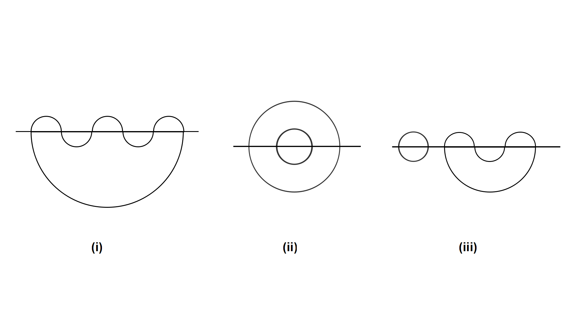
Figure 3: (i) 1-component meander of order 3; (ii) order 2, 2 components; (ii) order 3, 2 components

A multi-component meander is said to be $k$-reducible if a proper non-trivial collection of its connected components can be detached from the meander by cutting the river $k$ times between the bridges. Otherwise the meander is said to be $k$-irreducible.

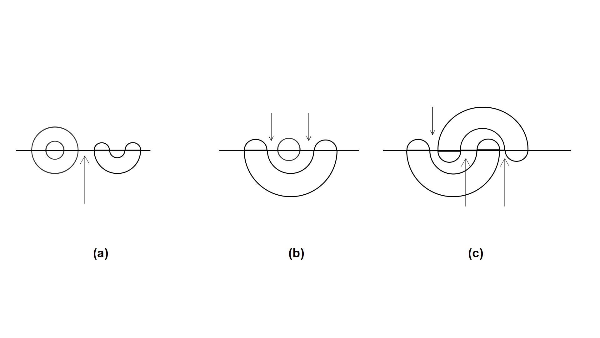
Figure 4: meanders that are (a) 1-reducible but 2-irreducible; (b) 1- and 2-reducible but 3-irreducible (c) 3-reducible

The 2-irreducible meanders have been studied extensively in [10] (where they are called irreducible meanders). Denote the generating series of the $q_{m}$ by $\mathcal{Q}$. Our connection to these objects is the following

Proposition 4.11.

Let $q_{n}$ denote the number of 2-irreducible meanders of order $2n$ and $k_{n}=k_{n}(\xi\otimes\eta)$ the $n^{\text{th}}$ cumulant of $\xi\otimes\eta$. Then

$$k_{n}(\xi\otimes\eta) =\begin{cases}q_{m}\quad&\text{if }n=2m\\ 0&\text{if }n\text{ is odd}\end{cases}$$ (4.12)

Proof.

We first prove by induction that $k_{n}=0$ if $n$ is odd, which will follow from the fact that $\widehat{\phi}((\xi\otimes\eta)^{n})=0$ for $n$ odd. Assume that $k_{m}=0$ whenever $m<n$ is odd. From (2.3) it follows that

$$k_{n} =\sum_{\begin{subarray}{c}\pi\in\operatorname*{NC}(n)\\ \pi\neq\mathbf{1}\end{subarray}}k_{\pi}$$

where $$k_{\pi}=k_{V_{1}}\ldots k_{V_{r}} V_{1},\ldots,V_{r} \pi \mathbf{1} [k]_{\mathbf{1}}=\underline{n} \pi\in\operatorname*{NC}(n)\setminus\{\mathbf{1}\} m m<n k_{m} k_{\pi} k_{m}=0 k_{n}=0$$ if are the equivalence classes of and denotes the identity partition, i.e. . Every must contain at least one equivalence class of size for some odd integer . Since is a factor of and , the inductive hypothesis implies as required. Hence

$$R_{\xi\otimes\eta}(z) =\sum_{n=1}^{\infty}k_{2n}z^{2n-1}.$$

Define the moment series of $$\xi\otimes\eta$$ by

$$M(z) =\frac{1}{z}G\left(\frac{1}{z}\right)=1+\sum_{n=1}^{\infty}\widehat{\phi}\left((\xi\otimes\eta)^{n}\right)\,z^{n}.$$

It is a consequence of the relationship between Cauchy and R-transform that

$$M(z) =1+zM(z)\,R(zM(z)).$$ (4.13)

We will introduce one more generating series. Put

$$\rho(z) =\sum_{n=1}^{\infty}q_{n}z^{2n-1}$$

so that $$\mathcal{Q}(z)=1+z\rho(z)$$. From (7.10) in [7] we have

$$M(z) =q(zM(z))=1+zM(z)\,\rho(zM(z)).$$ (4.14)

Combining (4.13) and (4.14) yields $\rho=R$ as power series. That $k_{2n}=q_{n}$ now follows from comparing coefficients. ∎

4.4 The Distribution of $Z(2\pi)$

So we have an explicit expression for the R-transform of $\xi\otimes\eta$. We will use this to obtain the R-transform of $Z(2\pi)$.

Recall that all odd cumulants of $\xi_{n}\otimes\eta_{n}$ and $\eta_{n}\otimes\xi_{n}$ vanish, hence the same is true of $Z(2\pi)$.

Proposition 4.15.

The $2n^{\text{th}}$ cumulant of $Z(2\pi)$ is $2\,\zeta(2n)\,q_{n}$ where $\zeta$ is the Riemann zeta function.

Proof.

Recall that $\zeta(m)=\sum_{n=1}^{\infty}n^{-m}$. So

$$R_{Z(2\pi)}(z) =2\sum_{n=1}^{\infty}\frac{1}{n}\,R_{\xi\otimes\eta}\left(\frac{z}{n}\right)=2\sum_{n=1}^{\infty}\frac{1}{n}\sum_{m=1}^{\infty}k_{m}\left(\frac{z}{n}\right)^{m-1}$$

$$=2\sum_{n=1}^{\infty}\sum_{m=1}^{\infty}n^{-2m}q_{m}z^{2m-1}$$

$$=\sum_{m=1}^{\infty}2\,\zeta(2m)q_{m}z^{2m-1}$$

where interchanging the sums over $m$ and $n$ is justified by absolute convergence. ∎

Definition 4.16 (see [16], p. 107).

Let $(a_{n})_{n\in\mathbb{N}}$, $(b_{n})_{n\in\mathbb{N}}$ be two sequences with generating functions $f,g$ respectively. The Hadamard product of $f,g$ is defined to be the generating function of $(a_{n}b_{n})$, denoted $f\boxast g$. That is

$$f\boxast g(z) =\sum_{n=1}^{\infty}a_{n}b_{n}z^{n}.$$

So $R_{Z(2\pi)}$ is twice the Haddamard product of the generating functions of the 2-irreducible meanders and that of the sequence $\{\zeta(2m)\colon m\in\mathbb{N}\}$.

From (6.3.14) in Abramowitz–Stegun [1] we have for $\left|z\right|<1$,

$$\sum_{n=2}^{\infty}\zeta(n+1)z^{n} =-\gamma-\Psi(1-z)$$

where $$\gamma \Psi$$ is the Euler constant and is the Digamma function defined by

$$\Psi(z) =\frac{\mathrm{d}}{\mathrm{d}z}\log\Gamma(z)=\frac{\Gamma^{\prime}(z)}{\Gamma(z)}.$$

Since the generating series can be considered as functions inside their radius of convergence, we can use complex analysis to compute their Hadamard product. Namely

Lemma 4.17.

Let $f,g$ be generating functions of $(a_{n})_{n\in\mathbb{N}}$, $(b_{n})_{n\in\mathbb{N}}$ and suppose that they are analytic on a neighbourhood of 0. Then

$$(f\boxast g)(z^{2}) =\frac{1}{2\pi i}\int_{\gamma}f(zw)\,g\left(\frac{z}{w}\right)\,\frac{\mathrm{d}w}{w}$$ (4.18)

on a neighbourhood $U$ of 0, where $\gamma$ is a smooth closed curve around 0 and contained in $U$.

Proof.

Let $U_{1},U_{2}$ be neighbourhoods of 0 on which $f$ and $g$ respectively are analytic. Then for $z\in U=U_{1}\cap U_{2}$,

$$\frac{1}{2\pi i}\int_{\gamma}f(zw)\,g\left(\frac{z}{w}\right)\,\frac{\mathrm{d}w}{w} =\left[f(z\eta)\,g\left(\frac{z}{\eta}\right)\right]_{\eta^{0}}$$

$$=\left[\sum_{n=0}^{\infty}a_{n}(z\eta)^{n}\sum_{m=0}^{\infty}b_{m}\left(\frac{z}{w}\right)^{m}\right]_{\eta^{0}}$$

$$=\left[\sum_{m,n}a_{n}b_{m}z^{n+m}\eta^{n-m}\right]_{\eta^{0}}$$

$$=\sum_{n=0}^{\infty}a_{n}b_{n}z^{2n}=f\boxast g(z^{2})$$

where $[\cdot]_{\eta^{0}}$ denotes the constant term in a Laurent series in $\eta$. ∎

Corollary 4.19.

Let $\epsilon\in(0,\rho)$ where $\rho$ is the radius of convergence of $R_{Z(2\pi)}$ and choose the canonical branch of the square root on $B(0,\rho)$. Then for $z\in B(0,\rho)$

$$R_{Z(2\pi)}(z) =-\frac{z^{1/2}}{\pi i}\int_{\Gamma}\Psi(1-z^{1/2}w)\,\mathcal{Q}\left(\frac{z}{w}\right)\,\mathrm{d}w$$ (4.20)

where $\Gamma=\partial B(0,\rho)$.

Proof.

By Proposition 4.15 we have $R_{Z(2\pi)}=2\,\mathcal{Q}\boxast\Lambda$ where, using (4.4)

$$\Lambda(z) =\sum_{n=1}^{\infty}\zeta(m)z^{m}=-z\Psi(1-z)-\gamma z.$$

Lemma 4.17 now yields

$$(\mathcal{Q}\boxast\Lambda)(z^{2}) =\frac{1}{2\pi i}\int_{\Gamma}\Lambda(zw)\,\mathcal{Q}\left(\frac{z}{w}\right)\,\frac{\mathrm{d}w}{w}$$

$$=-\frac{1}{2\pi i}\int_{\Gamma}zw\left(\Psi(1-zw)+\gamma\right)\,\mathcal{Q}\left(\frac{z}{w}\right)\,\frac{\mathrm{d}w}{w}$$

$$=-\frac{1}{2\pi i}\int_{\Gamma}z\Psi(1-zw)\,\mathcal{Q}\left(\frac{z}{w}\right)\,\mathrm{d}w$$

$$\quad-\frac{\gamma\,z}{2\pi i}\int_{\Gamma}\mathcal{Q}\left(\frac{z}{w}\right)\,\mathrm{d}w.$$

The argument of the integral in the second summand has a power series with only even powers of $$w$$ so the integral itself must vanish. We therefore have

$$(q\boxast\Phi)(z^{2}) =\frac{z}{2\pi i}\int_{\Gamma}\Psi(1-zw)\,q\left(\frac{z}{w}\right)\,\mathrm{d}w$$

∎

Remark 4.21.

In[7] it has been shown that the radius of convergence of $\mathcal{Q}$ is $\frac{4}{\pi}-1$. Since $\zeta(m)\longrightarrow 1$ as $m\longrightarrow\infty$, it follows that the radius of convergence of $R_{Z(2\pi)}$ is also $\frac{4}{\pi}-1$.

It is well-known, see [8], that the semicircular distribution is $\boxplus$-infinitely divisible. By Lemma 4.3 it follows that the $\xi_{n}\otimes\eta_{n}$ and $\eta_{n}\otimes\xi_{n}$ are $\boxplus$-infinitely divisible. Since free infinite divisibility is preserved by free linear combinations and weak limits, it follows that $Z(2\pi)$ is also $\boxplus$-infinitely divisible.

Unfortunately it seems that there is no explicit formula for $\mathcal{Q}$. It is therefore not apparent how a similar analysis to that for the square norm could be applied in order to obtain further details about the distribution of $Z(2\pi)$.

5 Lévy Area of the Free Brownian Bridge

In this section we use the Lévy representation

$$\beta(t)=\sum_{n=1}^{\infty}\frac{\cos(nt)-1}{n\sqrt{\pi}}\,\xi_{n} +\sum_{n=1}^{\infty}\frac{\sin(nt)}{n\sqrt{\pi}}\,\eta_{n}$$ (5.1)

of the free Brownian bridge to compute the distribution of the free analogue of the classical Lévy area process defined by

$$\mathcal{L}(t)=\frac{i}{2}\int_{0}^{t}\left[\beta(s),\mathrm{d}\beta(s)\right] =\frac{i}{2}\int_{0}^{t}\left(\beta(s)\mathrm{d}\beta(s)-\mathrm{d}\beta(s)\beta(s)\right).$$ (5.2)

When $$\beta \beta$$ is a two-dimensional commutative Brownian motion this is very similar to the object studied by Lévy[11]. By standard properties of the non-commutative integral [4] and self-adjointness of we have

$$\int_{0}^{t}\beta(s)\mathrm{d}\beta(s) =\left(\int_{0}^{t}\mathrm{d}\beta(s)\beta(s)\right)^{*}.$$

A straightforward calculation yields that the left hand side equals, for $$t=2\pi$$,

$$\int_{0}^{2\pi}\beta(s)\mathrm{d}\beta(s) =\sum_{n=1}^{\infty}\frac{1}{n}\left(\xi_{n}\eta_{n}-\eta_{n}\xi_{n}\right)$$ (5.3)

which is easily seen to be anti-self-adjoint. This is the reason for the factor of $i$ in (5.2): multiplying an anti-self-adjoint operator by $i$ yields a self-adjoint random variable whose distribution is therefore supported in $\mathbb{R}$. Thus $\mathcal{L}:=\mathcal{L}(2\pi)$ is equal to either side of (5.3) multiplied by $i$.

The summands are commutators of free semicircular random variables. Commutators have been studied by Nica–Speicher[13], where the semicircle distribution is discussed in Example 1.5(2). If $c_{n}=i\left(\xi_{n}\eta_{n}-\eta_{n}\xi_{n}\right)$, then the support of $\mu_{c_{n}}$ is $[-r,r]$ where $r=\sqrt{\frac{11+5\sqrt{5}}{2}}$ and

$$R_{c_{n}}(z) =\frac{2z}{1-z^{2}}=2\sum_{m=1}^{\infty}z^{2m-1}.$$ (5.4)

From this we can now compute the R-transform of the classical Lévy area. Let that function be denoted $R_{\mathcal{L}}$ then

$$R_{\mathcal{L}} =\sum_{n=1}^{\infty}\frac{1}{n}R_{c_{n}}\left(\frac{z}{n}\right)=\sum_{n=1}^{\infty}\frac{2n}{n^{2}-z^{2}}$$

$$=\frac{1}{z}-\pi\cot(\pi z).$$ (5.5)

We can deduce the free cumulants of $\mathcal{L}$, either from the Taylor series of (5.5) or by calculating

$$R_{\mathcal{L}} =\sum_{n=1}^{\infty}\frac{2}{n}\sum_{m=1}^{\infty}\left(\frac{z}{n}\right)^{2m-1}=\sum_{m=1}^{\infty}2\left(\sum_{n=1}^{\infty}n^{-2m}\right)\,z^{2m-1}$$

$$=\sum_{m=1}2\zeta(2m)z^{2m-1}$$

where the interchanging of the infinite sums is justified by absolute convergence. The free cumulants of $\mathcal{L}$ are therefore given by

$$k_{m}(\mathcal{L}) =\begin{cases}2\zeta(m)\quad&\text{if }m\text{ is even}\\ 0&\text{otherwise.}\end{cases}$$ (5.6)

Free infinite divisibility is characterised by an analytic property of the R-transform. An analytic function $f\colon\mathbb{C}^{+}\longrightarrow\mathbb{C}^{+}$ is called a Pick function. For $a,b\in\mathbb{R}$ with $a<b$ we denote by $\mathcal{P}(a,b)$ the set of Pick functions $f$ which have an analytic continuation $g\colon\mathbb{C}\setminus\mathbb{R}\cup(a,b)\longrightarrow\mathbb{C}$ such that $g(\overline{z})=\overline{g(z)}$. The following result is Theorem 3.3.6 of Hiai–Petz[8]:

Theorem 5.7.

A compactly supported probability measure $\mu$ is $\boxplus$-infinitely divisible if and only if its R-transform extends to a Pick function in $\mathcal{P}(-\epsilon,\epsilon)$ for some $\epsilon>0$.

It is easy to see that the common R-transform of the $c_{n}$ extends to a Pick function in $\mathcal{P}(-1,1)$. Therefore each $c_{n}$ is $\boxplus$-infinitely divisible.

Corollary 5.8.

The distribution of $\mathcal{L}$ is $\boxplus$-infinitely divisible.

As in Section 3 we can use free infinite divisibility together with the analytic properties of the R-transform and the formula for the maximum of the support from [15] to describe further the distribution in question.

The variational formula of Section 3 (Theorem 3.11) assumed that all free cumulants are positive, which is not the case for $\mathcal{L}$ (which is symmetric and therefore has vanishing odd free cumulants). However non-negativity of all free cumulants is actually enough [15, Theorem 5.9]:

Theorem 5.9.

Let $a\in\mathcal{A}$ be a self-adjoint non-commutative random variable with distribution $\mu$ and free cumulants $k_{m}\geq 0$ for all $m$. Then the right edge $\rho_{\mu}$ of the support of $\mu$ is given by

$$\log\left(\rho_{\mu}\right) =\sup\left\{\frac{1}{m_{1}(p)}\sum_{n\in L}p_{n}\log\left(\frac{k_{n}}{p_{n}}\right)-\frac{\Theta(m_{1}(p))}{m_{1}(p)}\colon p\in\mathfrak{M}_{1}^{1}(L)\right\}$$ (5.10)

where $\mathfrak{M}_{1}^{1}(L)$ denotes the set of $p\in\mathfrak{M}_{1}^{1}(\mathbb{N})$ such that $p(L^{c})=0$ and $\Theta$ was defined in Theorem 3.11.

The inverse of the Cauchy transform of $\mathcal{L}$ is given by

$$K_{\mathcal{L}} =R_{\mathcal{L}}+\frac{1}{z}=\frac{2}{z}-\pi\cot(\pi z).$$

We can check, by simple if lengthy computations similar to those in Section 3.2 that for every $t\in(\pi,2\pi)$ there exists unique $r(t)>0$ such that $\mathfrak{Im}\left[K_{\mathcal{L}}\left(r(t)e^{it}\right)\right]=0$ and that

$$\left.\frac{\partial}{\partial z}\mathfrak{Im}\left[K_{\mathcal{L}}(z)\right]\right|_{z=r(t)e^{it}} \neq 0\quad\quad\forall t\in(\pi,2\pi).$$ (5.11)

We obtain the following characterisation of the distribution of $\mathcal{L}$:

Proposition 5.12.

The non-commutative random variable $\mathcal{L}$ is distributed according to $\mu_{\mathcal{L}}(\mathrm{d}t)=\Phi_{\mathcal{L}}(t)\mathbf{1}_{[-\rho_{\mathcal{L}},\rho_{\mathcal{L}}]}\,\mathrm{d}t$ where $\Phi_{\mathcal{L}}(x)=-\frac{1}{\pi}r(t_{x})\sin(\tau_{x})$ and $\tau_{x}$ is the unique solution on $(\pi,2\pi)$ to

$$\frac{2}{r(\tau_{x})\,e^{i\tau_{x}}} -\pi\cot\left(\pi r(\tau_{x})\,e^{i\tau_{x}}\right)=x.$$ (5.13)

for every $$x\in(-\rho_{\mathcal{L}},\rho_{\mathcal{L}}) \rho_{\mathcal{L}}$$. The number is given by

$$\rho_{\mathcal{L}} =\frac{m_{*}\pi}{\sqrt{m_{*}^{2}-2}}$$ (5.14)

where $$m_{*} (\sqrt{2},\infty)$$ is the unique solution on of

$$m-2 =\sqrt{m^{2}-2}\,\cot\left(\frac{\sqrt{m^{2}-2}}{m-1}\right).$$ (5.15)

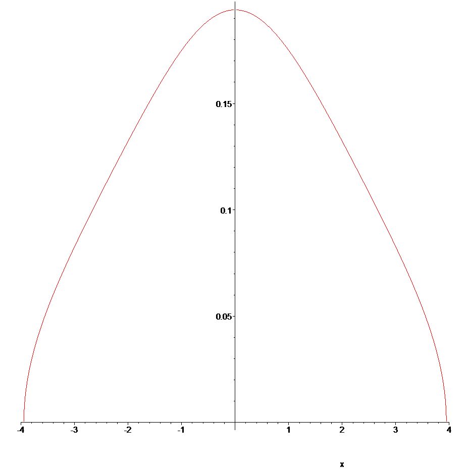
Density of the free Lévy area

Proof of Proposition 5.12.

The law $\mu_{\mathcal{L}}$ of $\mathcal{L}$ is symmetric about 0. Together with the analytic arguments of Section 3.2, suitably modified, this implies the existence of $\rho_{\mathcal{L}}>0$ such that the density $\Phi_{\mathcal{L}}$ of $\mu_{\mathcal{L}}$ is smooth, positive on $(-\rho_{\mathcal{L}},\rho_{\mathcal{L}})$ and zero everywhere else. The function $\Phi_{\mathcal{L}}$ is given by $\Phi_{\mathcal{L}}(x)=-\frac{1}{\pi}r(\tau_{x})\sin(\tau_{x})$ where $\tau_{x}$ is characterised by (5.13).

For the remainder of the statement we apply Theorem 5.9. Only the free cumulants of even order are nonzero, so that $L=\{2n\colon n\in\mathbb{N}\}$. The supremum on the right-hand side of (5.10) is attained by a unique maximiser which gives rise to equations (5.14) and (5.15). This completes the proof of the proposition. ∎

Mathematics Institute, University of Warwick, Coventry CV4 7AL, UK
 
Email address j.ortmann@warwick.ac.uk

References

- [1] Abramowitz, M., and Stegun, I. A., Eds. Handbook of Mathematical Functions. Dover Publications, 1965.
- [2] Bercovici, H., and Pata, V. Stable laws and domains of attraction in free probability theory. with an appendix by philippe biane. Annals of Mathematics 149 (1999), 1023 – 1060.
- [3] Bercovici, H., and Voiculescu, D. Free convolution of measures with unbounded support. Indiana University Mathematics Journal 42 (1993), 733 – 773.
- [4] Biane, P., and Speicher, R. Stochastic Calculus with Respect to Free Brownian Motion and Analysis on Wigner Space. Prob. Theory Rel. Fields 112 (1998), 373–409.
- [5] Bollobás, B. Linear Analysis, second ed. Cambridge University Press, 1999.
- [6] Capitaine, M., and Donati-Martin, C. The Lévy Area Process for the Free Brownian Motion. Journal of Functional Analysis 179 (2001), 153–169.
- [7] Francesco, P. D., Golinelli, O., and Guitter, E. Meander, Folding and Arch Statistics. Math.Comput.Modelling 26N8 26 (1997), 97–147.
- [8] Hiai, F., and Petz, D. The Semicircle Law, Free Random Variables and Entropy, vol. 77 of Mathematical Surveys and Monographs. American Mathematical Society, 2000.
- [9] Kac, M. On Some Connections Between Probability Theory and Differential and Integral Equations. Proceedings of the Second Berkeley Symposium on Mathematical Statistics and Probability (1950), 189 – 215.
- [10] Lando, S. K., and Zwonkin, A. Plane and Projective Meanders. Theoretical Computer Science 117 (1993), 227 – 241.
- [11] Lévy, P. Wiener’s Random Function, and Other Laplacian Random Functions. Proceedings of the Second Berkeley Symposium on Mathematical Statistics and Probability (1950), 171–187.
- [12] Lyons, T. Differential Equations Driven by Rough Signals. Revista Matématica Iberoamericana 14 (1998), 215–310.
- [13] Nica, A., and Speicher, R. Commutators of Free Random Variables. Duke Mathematical Journal 92, 3 (1998), 553–559.
- [14] Nica, A., and Speicher, R. Lectures on the Combinatorics of Free Probability. Cambridge University Press, 2006.
- [15] Ortmann, J. Large deviations for non-crossing partitions. In preparation.
- [16] Stanley, R. P. Enumerative Combinatorics, Volume 1, vol. 49 of Cambridge Studies in Advanced Mathematics. Cambridge University Press, 1997.
- [17] Tolmatz, L. On the Distribution of the Square Integral of the Brownian Bridge. Annals of Probability 30, 1 (2002), 253 – 269.
- [18] Victoir, N. Lévy Area for the Free Brownian Motion: Existence and Non-Existence. J. Funct. Anal. 208 (2004), 107 – 121.
- [19] Voiculescu, D. V. Lectures on Free Probability Theory. No. 1738 in Lecture Notes in Mathematics (Lectures on Probability and Theory and Statistics). Springer, 2000, pp. 283 – 349.
- [20] Voiculescu, D. V., Dykema, K. J., and Nica, A. Free Random Variables, vol. 1 of CRM Monograph Series. American Mathematical Society, 1992.