Variations of the coefficient $J_{2}$ of geopotential, and the dynamical Love number $k_{2}^{d}$ from the analysis of laser ranging to LAGEOS 1 and LAGEOS 2.

G.A.Krasinsky

Institute of Applied Astronomy, St. Petersburg, Russia, email: kra@quasar.ipa.nw.ru

Abstract Secular and seasonal variations of the coefficient $J_{2}$ of the geopotential are studied from the analysis of laser measurements of distances to the geodetic satellites LAGEOS 1 (1988–2003) and LAGEOS 2 (1992–2003). It is confirmed that beside the well-known annual variations with the amplitude $\approx 2.5\times 10^{-10}$ there also exist very significant semi-annual variations of a comparable amplitude. Phases of these two modes are such that the total effect may be described as a sharp postive splash of $J_{2}$ in August and considerably smaller variations in the rest part of year. The adopted theoretical value of the so-called dynamical Love number $k_{2}^{d}$ (a scale factor of near-diurnal oscillations aroused by the Earth’s fluid core in the coefficients $c_{2}^{1}$, $s_{2}^{1}$ of the geopotential) is improved applying a simple close form of these oscillations expressed in terms of the differential angular velocities $v_{1}$, $v_{2}$ of the fluid core. It is shown that this form is equivalent to the standard one of Fourier series in which such oscillations usually are referred to as a frequency-dependence of the Love number $k_{2}$. The derived estimate $k_{2}^{d}=0.0595\pm 0.0007$ statistically differs from the theoretical value $k_{2}^{d}=0.063$. Out-phase oscillation of $k_{2}^{d}$ with the period about 18.6 years and the amplitude $0.0064\pm 0.0011$ is detected giving evidence of large dissipation in the fluid core. The estimated secular trend $\dot{J}_{2}$ (commonly interpreted as the effect of the so-called Post-Glacial Rebound) appears twice less than the value recommended by the standards of the International Earth Rotation Service (IERS) but agrees with last findings of other authors.

Keywords: Earth’s satellites, geopotential, tides, Love numbers, SLR observations

1 Introduction

Starting point of this research was studying the near-diurnal oscillations $dc_{2}^{1}$, $ds_{2}^{1}$ caused by the Earth’s fluid core in the coefficients $c_{2}^{1}$, $s_{2}^{1}$ of geopotential. This effect (interpreted as the frequency-dependence of the Love number $k_{2}$) is presented by IERS standards in the form of the sum of trigonometric harmonics that depend on the fundamental arguments of the nutation theory (McCarthy, Petit, 2004). It may be shown that the amplitudes of these harmonics are proportional to the so-called dynamical Love number $k_{2}^{d}$. In Appendix, the expression for the corrections $dc_{2}^{1}$, $ds_{2}^{1}$ is derived in the simple close form:

$$\pmatrix{dc_{2}^{1}\cr ds_{2}^{1}\cr}=-\omega^{-1}J_{2}{k_{2}^{d}\over k_{s}}\pmatrix{v_{1}\cr v_{2}\cr},$$ (1)

where $v_{1}$, $v_{2}$ are the equatorial components of the angular velocity of the fluid core relatively to the Earth as a whole, $J_{2}$ is the coefficient of the second zonal harmonics of the geopotential, $\omega$ is the Earth angular velocity, $k_{s}=0.93831$ is the so-called secular Love number. It will be also shown that this presentation is equivalent to the standard form of trigonometric series for the frequency-dependence of the Love number $k_{2}$.

The parameter $k_{2}^{d}$ plays important role in two geodynamical problems. Firstly, it is rotation of the deformable Earth in the framework of the standard SOS model (Moritz, Muller, 1987), and secondly, dynamics of the Earth’s satellites. In short, perturbations of rotation of the deformable Earth depend on the so-called compliance $\xi$ that describes the tidal response of the moments of inertia of the Earth on the differential rotation of its fluid core. This parameter may be expressed in terms of the dynamical Love number $k_{2}^{d}$ by the relation $\xi=ek_{2}^{d}/k_{s}$ in which $e$ is the dynamical flattening of the Earth. Unfortunately, while processing Celestial Pole positions provided by geodetic VLBI observations it proved impossible to separate $k_{2}^{d}$ from the correction to the ratio of the moment of inertia of the fluid core to that of the Earth as a whole (Shirai, Fukushima, 2001), (Krasinsky, Vasilyev, 2006). On the other hand, the near-diurnal variations of the coefficients $c_{2}^{1}$, $s_{2}^{1}$ of the geopotential bring about accumulating secular effects in the node of satellite orbits and thus one may hope to estimate $k_{2}^{d}$ from satellite laser ranging (SLR) observations of geodetic satellites. As the adopted value of $k_{2}^{d}$ is purely theoretical, confronting it with experimental data is quite an actual problem. The value derived in this paper from the analysis of SLR data of the geodetic satellites LAGEOS 1 and LAGEOS 2 is, to our knowledge, a first experimental estimation of this parameter.

¿From the same analysis of the SLR data, we determine also corrections to the coefficient $J_{2}$ of the geopotential for studying the time-variability of this coefficient. In such a study, obtaining the secular trend $\dot{J}_{2}$ is a problem of primary importance as the IERS standards recommend to take this effect into account whenever numerical integration of the equations of artificial satellite motion has to be done. At present, two centers of analysis (University of Texas and Goddard Space Flight Center) are monitoring the geopotential on a regular basis. Recent publications of the first group (Cheng, Tapley, 2008) and the second one (Lemoine et al., 2006) have revealed serious discrepancies between the derived values of the secular trend: $\dot{J}_{2}=-2.6\times 10^{-11}\mbox{/year}$ and $\dot{J}_{2}=-1.3\times 10^{-11}\mbox{/year}$, correspondingly. So, the independent study of $\dot{J}_{2}$ documented in Section 3.3 seems to be actual.

2 Observations and their processing

We have used the laser observations of the geodetic satellites LAGEOS 1 (1988–2003), and LAGEOS 2 (1992–2003) taken from the server ftp://cddis.nasa.gov. The observations of each year were combined into one series and treated simultaneously. In Tab.1, the following information on the observations is given for each year: their total number $N_{obs}$, the total number $N_{del}$ of rejected observations, the Weighted Root Mean Square (WRMS) error of one-way distances to the satellite (in millimeters). Six orbital elements of the satellite under study and two dynamical empirical terms (along- and cross-track perturbing accelerations) were estimated weekly as local parameters. When processing the observations of each year, these local parameters were determined simultaneously with the global ones which are the coordinates of observing stations and the value of the dynamical Love number $k_{2}^{d}$. In addition, on each monthly interval (more exactly, on the interval of four weeks) a correction to the coefficient $J_{2}$ of the geopotential also was determined for further study of its time variations. It is known that SLR observations made in different stations are of quite various quality. Properly down-weighted or rejected, the observations of poor quality do not distort the resulting estimates. In fact, only few stations of the last generation provide the overwhelming volume of high precision data that affect the results.

As an example, from the typical set of the observations of LAGEOS 1 of the year 2000, the following parameters have been derived:

• dynamical Love number $k_{2}^{d}$,

• monthly corrections to $J_{2}$ (13 unknowns),

• weekly corrections to six elements of the satellite and two empirical parameters ($52\times 8=416$ unknowns),

• yearly corrections to the coordinates of 99 stations (295 unknowns).

Thus, the total number of the estimated parameters for this year is 626. Values of the longitudes and latitudes of several fiducial stations (which provide the bulk of accurate observations) have been fixed to prevent degeneration of the normal matrix due to correlations with the elements of orientation of the satellite orbit. The software complex ERA for ephemeris and dynamical astronomy was applied while constructing the numerical theories of the orbital motion, calculating the theoretical distances to the satellites and processing the condition equations. The current DOS and Windows versions are available from the anonymous FTP server quasar.ipa.nw.ru/incoming/era. All calculations are carried out in accordance with the recommendations of IERS 2003 conventions (McCarthy, Petit, 2004). The only difference in the dynamical equations of the satellite motion is making use of the close form (1) for the corrections $dc_{2}^{1}$, $ds_{2}^{1}$ caused by the fluid core. We will show that this approach is equivalent to that recommended by IERS but is more convenient because the functional dependence of the perturbing forces on $k_{2}^{d}$ is presented in explicit form.

Table 1: WRMS errors $\sigma$ of the post-fit residuals (mm)

		LAGEOS 1			LAGEOS 2
Year	$N_{obs}$	$N_{del}$	$\sigma(mm)$	$N_{obs}$	$N_{del}$	WRMS $(mm)$
1988	67414	3058	22
1989	64030	3411	22
1990	77951	2721	22
1991	54981	3518	22
1992	59715	6073	24	13683	863	21
1993	81398	7665	22	78873	7128	22
1994	65370	4990	27	66827	4557	21
1995	53463	4353	24	52153	3183	20
1996	52725	4196	23	52244	7904	23
1997	50404	3336	22	53516	3688	17
1998	65010	5361	19	60819	3298	17
1999	71788	4693	23	66520	3415	18
2000	61888	4122	23	63158	2362	19
2001	71839	4060	19	70449	3083	19
2002	70780	2503	21	64011	2217	18
2003	74969	2379	19	74613	2798	19

3 Results of data processing

3.1 Dynamical Love number $k_{2}^{d}$

Applying the method described above, we have obtained the set of 16 yearly estimates of $k_{2}^{d}$ from the observations of LAGEOS 1 (1988–2003) and 12 estimates from LAGEOS 2 (1992–2003). They are presented in Fig.1 (the black circles correspond to LAGEOS 1, the hollow ones to LAGEOS 2). Generally, all the estimates are in a very good accordance (the only exception is the LAGEOS 1 result for the year 1995 which evidently drops out and thus has not been used). From this set, the following averaged value of the dynamical Love number is derived

$$k_{2}^{d}=0.0595\pm 0.0007$$

that statistically differs from the theoretical a priory value $k_{2}^{d}=0.063$ given in (Moritz, Muller, 1987).

Fig.1 demonstrates also an out-phase oscillation with the period 18.6 years and the amplitude $0.0064\pm 0.0011$. Probably, that is evidence of large dissipation in the fluid core. Note that parameters of the dissipative effects in the fluid core recommended by IERS standards are purely theoretical, and their numerical values have not yet been verified by observations.

Figure 1: Yearly estimates of dynamical Love number $k_{2}^{d}$

For checking a possible dependence of $k_{2}^{d}$ on its starting value, the observations of an arbitrarily chosen year were processed with the zero starting value of $k_{2}^{d}$. After several iterations, the resulted estimate appeared the same.

Note that in the methodically correct approach, the standard ”static” Love number $k_{2}$ should also be estimated from the analysis of SLR data. At present, the most accurate and reliable estimate of $k_{2}$ might be obtained from the analysis of geodetic VLBI observations. Using these data, the following consistent estimates have been derived: $k_{2}=0.2788\pm 0.0011$ (Shirai, Fukushima, 2001) and $k_{2}=0.27272\pm 0.00036$ (Krasinsky, Vasilyev, 2006) which are significantly less than the adopted value $k_{2}=0.3$. The error of this value may distort results of processing the SLR data.

3.2 Periodic variations of the coefficient $J_{2}$ of geopotential

Fig.2 presents the monthly corrections to $J_{2}$. The noticeable positive trends means that the a priory value $\dot{J}_{2}=-26\times 10^{-12}/\mbox{year}$ used in our calculations should be considerably diminished. When comparing Fig.2 with the analogous plots in (Cheng, Tapley, 2004) and (Cox et al, 2005) it is necessary to bear in mind that Fig.2 presents corrections to the assumed IERS value of $\dot{J}_{2}$ while those in the cited works correspond to the zero value of it. More details concerning the value $\dot{J}_{2}$ are discussed in the next section.

Methodically correct estimates of $\dot{J}_{2}$ may be derived only simultaneously with determination of cosine and sine coefficients of the main harmonics of the trigonometric polynomial approximation of $J_{2}$. These are the annual harmonics $A_{\cos}$, $A_{\sin}$, the semi-annual harmonics $A_{\cos}^{(0.5)}$, $A_{\sin}^{(0.5)}$, the harmonics $A_{\cos}^{\Omega}$, $A_{\sin}^{\Omega}$ connected with the period 18.6 year of revolution of the lunar node $\Omega$, and the empirical harmonics $A_{\cos}^{(3)}$, $A_{\sin}^{(3)}$ with the period of 3 year. We also estimated the correction $dJ_{2}(0)$ to the value $J_{2}$ for 2000.0. Four solutions are obtained for different sets of the estimated parameters (see Tab.2). The first column of Tab.2 specifies parameters under estimation, others give their estimated values. For the secular trend, there are given both the correction $d\dot{J}_{2}$ to the a priory value $-26\times 10^{-12}\mbox{/year}$, and the full value $\dot{J}_{2}$.

Tab.2 demonstrates that the estimates of the annual and semi-annual harmonics are robust and only slightly depend on the solutions. For the annual oscillations, the results can be compared with those by other authors. The full amplitude of the annual oscillations is $(229\pm 23)\times 10^{-12}$ in accordance with the value $300\times 10^{-12}$ taken approximately from Fig.1 of (Cox et al., 2005). Similar results are obtained in a number of other works; for instance, in (Cheng, Tapley, 2004) the seasonal amplitude is $290\times 10^{-12}$ (no error is given). The phases of the oscillations also agree: the negative minimum in January and the positive maximum in July. The amplitudes of the semi-annual oscillations are rather significant and comparable with those of the annual ones. The derived amplitudes of the semi-annual variations are consistent with the results published by other authors. For instance, Table 1 of paper (Nerem et al, 2006.) gives the estimated cosine and sine amplitudes of the semi-annual variations as $-2.41\times 10^{-10}$ and $0.78\times 10^{-10}$ in accordance with our findings (see Table 2).

The solid curve in Fig.2 presents Solution 4 (with maximal number of estimated parameters). Fig.2 shows that the seasonal variations cannot be described as a simple harmonic oscillation but have more complex structure. Namely, they keep near constant value from the beginning of every year till August when a sharp maximum takes place, and then decrease up to the end of the year. The plot given by Fig.2 is very similar to the intra-annual variations of $J_{2}$ presented by Fig 3(a) of (Moor et al. 2006) and derived from Lageos 1,2 data for the time span 1998-2004. Such behavior is a consequence of the large value of the semi-annual amplitude. This feature of the intra-annual variations qualitatively agrees with Fig.3 of paper (Lemoine et al. 2006) where they are presented for the interval 2000–2007 being derived from SLR data for 9 satellites combined with DORIS data. Note that Fig.3 in (Lemoine et al. 2006) presents variations of the coefficient $c_{20}=-J_{2}$. It is interesting that Fig.2 of the same paper does not demonstrate the fine structure of the intra-annual variations, probably because time-intervals between the consequent samples are two months (though the caption indicates one month, probably erroneously). With so low time resolution, the fine structure of the intra-annual variations cannot be discerned. Supposedly, this fine structure is due to the seasonal asymmetry of ice cover developing in the southern and northern semi-spheres. For a more detailed study of these variations, Fig.3 presents them vs. JD (mod 365.25) after removing the secular and long-periodic variations taken from Tab.2. Beside the maximum in August, this plot demonstrates also and l ong-periodic variations taken from Tab.2. Beside the maximum in August, this plot demonstrates also two small minima at April and November. Here only the LAGEOS 2 results have been used as the more accurate ones. The bars present statistical errors obtained after averaging 13 groups of the monthly estimates $J_{2}$ for all the years.

In Solutions 3 and 4, the sine and cosine components of the oscillation with the period 18.6 years have also been estimated (with the resulted WRMS errors considerably decreased). The nature of the empirical oscillation of the 3-year period estimated in Solution 4 is unclear. We tried several empirical long-periodic harmonics but statistically significant amplitudes were found only for the 3-year period.

Fig.2 demonstrates that the positive outliers correspond to the August spikes. It means that the values of these sharp spikes vary with time and cannot be presented by the simple model as the sum of the annual and semi-annual oscillations. Probably, this effect should admit some geophysical interpretation.

In the last two lines of Tab.2, the WRMS errors of the residuals are presented (both for LAGEOS 1 and LAGEOS 2). Note that the WRMS errors for LAGEOS 2 are considerably smaller than those for LAGEOS 1. Formal erors of $J_{2}$ appeared to be by order less than the range of the fluctuations of $dJ_{2}$, and so could not be presented by error bars in Fig.2.

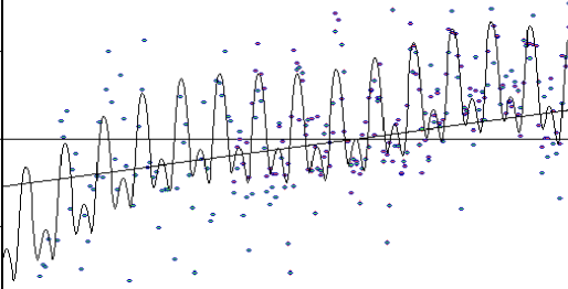
Figure 2: Corrections to the nominal $J_{2}$ (for the adopted $\dot{J}_{2}$) in $10^{-10}$

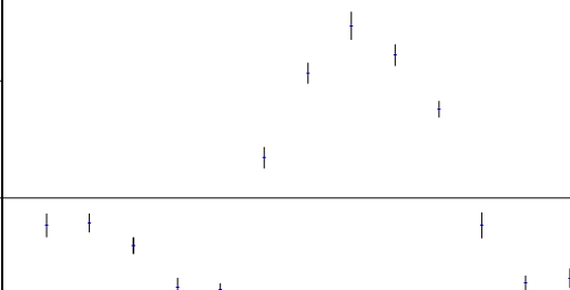
Figure 3: Intra-annual variations of $J_{2}$ vs. JD (mod 365.25) (in $10^{-11}$)

Table 2: Models of variations of $J_{2}$, four solutions (in $10^{-12}$)

	1	2	3	4
$dJ_{2}(0)$	218(16)	215(14)	103(31)	77(33)
$d\dot{J}_{2}/\mbox{year}$	33(3)	35(3)	18(7)	13(7)
$\dot{J}_{2}/\mbox{year}$	7(3)	9(3)	-8(7)	-13(7)
$A_{\cos}$	-172(19)	-174(17)	-184(15)	-183(15)
$A_{\sin}$	-151(19)	-150(16)	-164(15)	-168(15)
$A_{\cos}^{(0.5)}$		66(16)	67(15)	66(15)
$A_{\sin}^{(0.5)}$		167(17)	168(15)	168(15)
$A_{\cos}^{\Omega}$			154(39)	181(40)
$A_{\sin}^{\Omega}$			-102(20)	-98(20)
$A_{\cos}^{(3)}$				-43(15)
$A_{\sin}^{(3)}$				-39(16)
WRMS, LAGEOS 1	285	255	245	235
WRMS, LAGEOS 2	195	155	135	135

3.3 Secular trend $\dot{J}_{2}$ and the post-glacial rebound

True value of the trend $\dot{J}_{2}$ is quite important as for practical applications as for a geophysical interpretation. Indeed, the estimate $\dot{J}_{2}=-2.6\times 10^{-11}/\mbox{year}$ is still recommended by IERS standards (McCarthy, Petit, 2004) as experimentally confirmed effect of the post-glacial rebound, despite that this trend has greatly diminished or even completely vanished for the SLR data after 1998 (Cheng, Tapley, 2004). For instance, Fig.3 in (Chao, 2003) shows that the accumulated error of $J_{2}$ becomes intolerably large at present epoch if one applies the adopted value of $\dot{J}_{2}$. In recent publication (Cheng, Tapley, 2008), the authors insist that this value is still valid and explain the clearly seen deviations of $J_{2}$ from observations after 1998 by some decadal variations, making stress on the effect of El Niño. On the other hand, the independent analysis carried out in Goddard Space Flight Center (Lemoine et al, 2006) demonstrates that the time-behavior of $J_{2}$ was rather stable since 1976 up to 2007 with no noticeable change of it after 1998. The resulting value $\dot{J}_{2}=-1.32\times 10^{-11}$/year is twice less than that of the IERS standards based on the works by Cheng and Tapley. Our analysis of SLR data confirms this conclusion. In Solution 4 (maximal numbers of the estimated harmonics in $J_{2}$) we have obtained the estimate $\dot{J}_{2}=(-1.3\pm 0.7)\times 10^{-11}$/year which is consistent with the result of (Lemoine et al, 2006). Unfortunately, due to the comparatively short 16-yearly time-interval of the data used, the correlations of the amplitudes of the long-term variations with the secular trend are rather large. That is why the statistical error of our estimate of $\dot{J}_{2}$ is comparatively large. In any case, we may state that our value of $\dot{J}_{2}$ rules out the rate $-2.6\times 10^{-11}/\mbox{year}$ recommended by IERS standards.

4 Concluding notes

1. From the practical point of view, the most important result of this study is the conclusion that the derived secular trend $\dot{J}_{2}$ is consistent with the result of (Lemoine et al, 2006) confirming that the value of this trend recommended by IERS standards is twice too large. To our opinion, poor predictability of the variations of $J_{2}$ due to inter-annual oscillations of unclear origin necessitates monitoring of the current values of $J_{2}$ and disseminating the results for practical applications, just as at present it is done for the Earth’s orientation parameters.

2. The intra-annual variations of $J_{2}$ are not a simple harmonic oscillation; see Fig.3. Probably, the sharp spike in August is due to asymmetric seasonal developing of the ice regime in the southern and northern semi-spheres. This problem deserves thorough study and a geophysical interpretation.

3. The derived estimate $k_{2}^{d}=0.0595\pm 0.0007$ statistically differs from its theoretical value $k_{2}^{d}=0.063$. To our knowledge, that is the first experimental determination of this parameter.

4. For independent calculation of various tidal effects caused by the fluid core, it is desirable to provide users by numerical values of the angular velocities $v_{1},v_{2}$ of the fluid core. To avoid somewhat bulky analytical manipulations directly in the text of present paper, derivation of the analytical expressions for $v_{1},v_{2}$ is transferred into Appendix.

5 Appendix. Dynamical Love numbers

It is known that the positions of sites on the Earth’s surface are displaced by the pole tides of two types. Those of the first type are caused by the motion of the pole of the Earth as a whole, the corresponding tidal amplitudes being proportional to the Love numbers $h_{2}$, $l_{2}$. The pole tides of the second type are caused by the differential rotation of the fluid core relatively to the mantle; their amplitudes are proportional to the so-called dynamical Love numbers $h_{2}^{d}$, $l_{2}^{d}$. The pole tides of the both types also contribute to the tesseral coefficients $c_{2}^{1}$, $s_{2}^{1}$ of the geopotential. Putting aside the Chandler’s free wobble of the pole, these contributions are of near-diurnal periods with the amplitudes proportional either to the static ”potential” Love number $k_{2}$ or to the dynamical Love number $k_{2}^{d}$, the latter effect being the largest. A theory of the dynamical Love numbers is given in monograph (Moritz and Muller, 1987).

As the fluid core brings about diurnal oscillations of the coefficients $c_{2}^{1}$ and $s_{2}^{1}$ of the geopotential, it gives rise to rather significant long-term and secular perturbations in the elements of the observed satellites (mainly in the node) thus making it possible to improve the adopted theoretical value of the scaling factor $k_{2}^{d}$ of these perturbations. It is commonly assumed that the fluid core rotates relatively to the mantle with the angular velocity $\overline{v}=(v_{1},v_{2},0$), the equatorial components $v_{1},v_{2}$ being given by the theory of the Earth’s rotation. We denote $\overline{\omega}=(\omega_{1},\omega_{2},\omega_{3})$ the vector of the angular velocity of the Earth as a whole. For calculating the potentials $dW_{v}$ induced by the centrifugal acceleration of the differential rotation of the fluid core, the velocity of any point $\overline{r}$ in these two domains within the Earth (the mantle and fluid core) may be presented either as $\overline{\omega}\times\overline{r}$ or as $(\overline{\omega}+\overline{v})\times\overline{r}$, respectively. Then the centrifugal acceleration $\overline{W}$ within the mantle may be presented as

$$\overline{W}=-\overline{\omega}\times\left(\overline{\omega}\times\overline{r}\right)=-\overline{\omega}(\overline{r},\overline{\omega})+\overline{r}\omega^{2},$$

while in the fluid core the corresponding expression has the form

$$\overline{W}=-(\overline{\omega}+\overline{v})\times\left[(\overline{\omega}+\overline{v})\times\overline{r}\right]=-(\overline{\omega}+\overline{v})\left[(\overline{r},\overline{\omega})+(\overline{r},\overline{v})\right]+\overline{r}|\overline{\omega}+\overline{v}|^{2}$$

with the standard notations $(\overline{p},\overline{q})$ and $\overline{p}\times\overline{q}$ for the scalar and vectorial products of two vectors $\overline{p}$, $\overline{q}$.

The terms along the vector $\overline{r}$ in these expressions do not deform the incompressible Earth and may be disregarded. Then ignoring the second-order terms, we can set $\overline{W}=\mbox{grad}\ W$, the potential $W$ at the right part being given by the expressions

$$W=\left\{\begin{array}[]{l}-{1\over 2}(\overline{r},\overline{\omega})^{2},\ R_{c}<r<R,\\ -{1\over 2}(\overline{r},\overline{\omega})^{2}-(v_{1}x_{1}+v_{2}x_{2})x_{3}\omega,\ r<R_{c},\end{array}\right.$$ (4)

with the notations $R$, $R_{c}$ for the radii of the Earth and its fluid core, respectively.

Adding the spherically symmetric term ${3\over 2}r^{2}\omega^{2}$ to the right part (that does not affect the distribution of the density within the incompressible Earth) and denoting $\cos S=(\overline{\rho},\overline{\omega})/\omega$, $\overline{\rho}=\overline{r}/r$, we can present the potential $W$ in each of these two domains within the Earth as the following combinations of the zonal and tesseral harmonic functions:

$$W=\left\{\begin{array}[]{l}-{1\over 3}\omega^{2}r^{2}P^{0}_{2}(\cos S),\ R_{c}<r<R,\\ -{1\over 3}\omega^{2}r^{2}P^{0}_{2}(\cos S)-(v_{1}x_{1}+v_{2}x_{2})x_{3}\omega,\ R<R_{c}\end{array}\right.$$

In accordance with the general theory of Love numbers, action of the perturbing spherical harmonics deforms the Earth’s interior and the resulting deformations induce the additional potential $dW$ given on the Earth’s spherical surface (of the mean radius $R$) by the expression

$$dW|{R} = -{k_{2}\over 3}\omega^{2}R^{2}P^{0}_{2}(\cos S)-k_{2}^{d}R^{2}(v_{1}\rho_{1}+v_{2}\rho_{2})\rho_{3}\omega,$$ (6)

in which $k_{2},k_{2}^{d}$ are the standard static and dynamic Love numbers, $\overline{\rho}=\overline{r}/r=(\rho_{1},\rho_{2},\rho_{3})$ is the unit vector to the probing point out of the Earth. In the outer space, the first term at the right part generates the additional potential $dW_{r}$

$$dW_{r}=-{1\over 3}k_{2}\omega^{2}{R^{5}\over r^{3}}P^{0}_{2}(\cos S),\ r\geq R$$ (7)

which is the result of the tides aroused by rotation of the Earth as a whole, while the second term (proportional to $k_{2}^{d}$) brings about the tidal potential $dW_{v}$ caused by the differential rotation of the fluid core. The potential $dW_{v}$ has the form of the second-order tesseral harmonics:

$$dW_{v} = -k_{2}^{d}{R^{5}\over r^{3}}(v_{1}\rho_{1}+v_{2}\rho_{2})\rho_{3}\omega,\ r>R.$$ (8)

For our aims, the zonal part of the potential (7) may be ignored as it generates nothing but the permanent tidal component of $J_{2}$. Thus retaining only the tesseral terms (and keeping the old notation $dW_{r}$) we obtain

$$dW_{r} = -k_{2}{R^{5}\over r^{3}}(\omega_{1}\rho_{1}+\omega_{2}\rho_{2})\rho_{3}\omega,\ r>R.$$ (9)

Both these potentials, $dW_{r}$ and $dW_{v}$, should be added to the geopotential $V$ which may be written in the standard form

$$V={Gm\over r}\sum_{k,j}\left({R\over r}\right)^{k}P_{k}^{j}(\cos\delta)(c_{k}^{j}\cos j\lambda+s_{k}^{j}\sin j\lambda),$$ (10)

where $\delta,\lambda$ are the latitude and longitude of the probing point, $P_{k}^{j}$ are associated Legendre functions. In order to present potentials (8) and (9) in the similar form, the combinations $\rho_{1}\rho_{3},\rho_{2}\rho_{3}$ also should be expressed in terms of the associated Legendre functions:

$$\rho_{1}\rho_{3} = \cos\delta\sin\delta\cos\lambda={1\over 3}P_{2}^{1}(\cos\delta)\cos\lambda,$$

$$\rho_{2}\rho_{3} = \cos\delta\sin\delta\sin\lambda={1\over 3}P_{2}^{1}(\cos\delta)\sin\lambda,$$

and then we obtain

$$dW_{v}=-k_{2}^{d}\left({\omega R^{2}\over 3}\right)\left({R\over r}\right)^{3}P_{2}^{1}(\cos\delta)(v_{1}\cos\lambda+v_{2}\sin\lambda).$$

Defining the so-called secular Love number $k_{s}$ in the standard way

$$k_{s}=3{GmJ_{2}\over R^{3}\omega^{2}},$$

the expression for $dW_{v}$ may be re-written in the form

$$dW_{v}=-{Gm\over r}\left({R\over r}\right)^{2}\left({k_{2}^{d}\over k_{s}}\right)J_{2}P_{2}^{1}(\cos\delta)(v_{1}\cos\lambda+v_{2}\sin\lambda)/\omega.$$ (11)

Such a presentation of the potential $dW_{v}$ demonstrates that its contribution into geopotential (10) has the form of corrections $dc_{2}^{1}$, $ds_{2}^{1}$ to the coefficients $c_{2}^{1}$, $s_{2}^{1}$. These corrections may be written in the simple form:

$$\pmatrix{dc_{2}^{1}\cr ds_{2}^{1}\cr}=-J_{2}\omega^{-1}{k_{2}^{d}\over k_{s}}\pmatrix{v_{1}\cr v_{2}\cr}.$$ (12)

The analogous expression is valid for the corresponding corrections $dc_{2}^{1}$, $ds_{2}^{1}$ proportional to $k_{2}$:

$$\pmatrix{dc_{2}^{1}\cr ds_{2}^{1}\cr}=-J_{2}\omega^{-1}{k_{2}\over k_{s}}\pmatrix{\omega_{1}\cr\omega_{2}\cr}.$$ (13)

In this relation we only account for the components due to the forced variations of $\omega_{1}$, $\omega_{2}$ (the so-called Oppolzer’s terms) omitting the free Chandler’s oscillation which is of much longer period. Hereinafter, the components of the near-diurnal oscillations in $c_{2}^{1}$, $s_{2}^{1}$ proportional to $k_{2}$ will be referred to as the Oppolzer’s tides.

One can see that the variables $v_{1},v_{2}$ and $\omega_{1},\omega_{2}$ in the right parts of relations (12) and (13) indeed oscillate with near-diurnal periods. For instance, the angular velocities $\omega_{1},\omega_{2}$ in expression (13) may be presented in terms of the sidereal time $s$ and the time derivatives of the slowly changing angles of precession $\phi$ and nutation $\theta$ by the Euler’s kinematic relations:

$$\omega_{1} = \phantom{-}\dot{\theta}\cos s+\dot{\phi}\sin\theta\sin s,$$

$$\omega_{2} = -\dot{\theta}\sin s+\dot{\phi}\sin\theta\cos s.$$ (14)

In analogous way, the components $v_{1},v_{2}$ of the angular velocity of the fluid core may be transformed from the Earth-fixed frame into its components $n_{1}$, $n_{2}$ in the inertial frame:

$$v_{1} = \phantom{-}n_{1}\cos s+n_{2}\sin s$$

$$v_{2} = -n_{1}\sin s+n_{2}\cos s.$$ (15)

Slowly changing variables $n_{1},n_{2}$ can be expressed in terms of the nutational coefficients (and of the precession rate) making use of the differential equations of rotation of the deformable Earth with the fluid core; see (Moritz and Muller, 1987).

If dissipation in the fluid core is taken into consideration, the variables $v_{1},v_{2}$ should be calculated for the delayed time $t-\tau$. With all necessary accuracy, the linearized relations $v_{1}(t-\tau)=v_{1}(t)-\tau\dot{v}_{1}$ and $v_{2}(t-\tau)=v_{1}(t)-\tau\dot{v}_{2}$ may be applied. Moreover, to calculate the time-delayed variables $v_{1}$, $v_{2}$, one can take into account only the time delay in the sidereal time $s$ replacing in expression (12) $v_{1}$ by $v_{1}-v_{2}\delta$ and $v_{2}$ by $v_{2}+v_{1}\delta$ ($\delta=\tau\omega$ is the tidal phase lag). The dissipation brings about out-of-phase terms in the trigonometric presentation of the tidal effects. In the IERS standards, they are given for a theoretical value of the phase lag which, unfortunately, has not yet been verified by satellite data.

Perturbing potential (4) of the centrifugal accelerations brings about not only the near-diurnal tidal variations (12), (13) of the tesseral coefficients $c_{2}^{1}$, $s_{2}^{1}$ of the geopotential, but also near-diurnal displacements of sites: $dH$, $dN$, $dE$ in the radial, northern and eastern directions, respectively. In our notations, the displacements caused by the fluid core may be written in the form

$$dH = -R\left({h_{2}^{d}\over k_{s}}\right)J_{2}\sin 2\delta(v_{1}\cos\lambda+v_{2}\sin\lambda)/\omega,$$

$$dN = -R\left({l_{2}^{d}\over k_{s}}\right)J_{2}\cos 2\delta(v_{1}\cos\lambda+v_{1}\sin\lambda)/\omega,$$ (16)

$$dE = -R\left({l_{2}^{d}\over k_{s}}\right)J_{2}\sin\delta(-v_{1}\sin\lambda+v_{2}\cos\lambda)/\omega,$$

where $\lambda$, $\delta$ are the longitude and latitude of the site, $h_{2}^{d}$, $l_{2}^{d}$ are the dynamical Love numbers.

The tidal displacements due to the centrifugal potential of the Earth as a whole may be obtained replacing the dynamical Love numbers $h_{2}^{d}$, $l_{2}^{d}$ by the static Love numbers $h_{2}$, $l_{2}$ and the angular velocities $v_{1}$, $v_{2}$ of the differential rotation of the fluid core by the absolute angular velocities $\omega_{1}$, $\omega_{2}$. Broken into the trigonometric series of the fundamental arguments, the corrections (12), (16) are interpreted in the IERS standards (McCarthy, Petit, 2004) as the effect of the frequency-dependence of the Love numbers $k_{2}$ (or rather $k_{21}$), $h_{2}$ and $l_{2}$. It will be shown that the explicit analytical expressions of these trigonometric series have the following simple form (the proof is given at the end of Appendix):

$$dH = -R\left({h_{2}^{d}\over k_{s}}\right)J_{2}\sin 2\delta\sum_{\nu}(C_{\nu}\cos\lambda+S_{\nu}\sin\lambda),$$

$$dN = -R\left({l_{2}^{d}\over k_{s}}\right)J_{2}\cos 2\delta\sum_{\nu}(C_{\nu}\cos\lambda+S_{\nu}\sin\lambda),$$ (17)

$$dE = -R\left({l_{2}^{d}\over k_{s}}\right)J_{2}\sin\delta\sum_{\nu}(-C_{\nu}\sin\lambda+S_{\nu}\cos\lambda),$$

$$\pmatrix{dc_{2}^{1}\cr ds_{2}^{1}\cr}=-J_{2}\omega^{-1}\left({k_{2}^{d}\over k_{s}}\right)\sum_{\nu}\pmatrix{C_{\nu}\cr S_{\nu}\cr},$$ (18)

where

$$S_{\nu} = Q_{\nu}^{+}\sin(s+f_{\nu})+Q_{\nu}^{-}\sin(s-f_{\nu}),$$ (19)

$$C_{\nu} = Q_{\nu}^{+}\cos(s+f_{\nu})+Q_{\nu}^{-}\cos(s-f_{\nu})$$ (20)

for $\nu\neq 0$,

$$S_{0} = Q_{0}\sin(s)$$

$$C_{0} = Q_{0}\cos(s),$$

$s$ is the sidereal time, $f_{\nu}$ is the nutation argument of the frequency $\nu$ in the nutational series given by the expressions

$$\theta = \sum_{\nu\neq 0}\delta\theta_{\nu}\cos f_{\nu},$$ (21)

$$\psi = \sum_{\nu\neq 0}\delta\psi_{\nu}\sin f_{\nu},$$ (22)

$\delta\theta_{\nu},\delta\psi_{\nu}$ are coefficients of the nutations in inclination and longitude, and the coefficients $Q_{\nu}^{+}$, $Q_{\nu}^{-}$, $Q_{0}$ are expressed in terms of $\delta\theta_{\nu},\delta\psi_{\nu}$ by the relations

$$Q_{\nu}^{+} = (\delta\theta_{\nu}-\sin\theta_{0}\delta\psi_{\nu})q_{\nu},$$ (23)

$$Q_{\nu}^{-} = (\delta\theta_{\nu}+\sin\theta_{0}\delta\psi_{\nu})q_{-\nu},$$ (24)

$$Q_{0} = -{p\over\nu_{c}}\sin\theta_{0}(1-\kappa),$$ (25)

with the notations

$$q_{\nu} = {\nu\over\nu_{c}+\nu}(1-\kappa),\quad\nu\neq 0,$$ (26)

$$\kappa = \left({k_{2}^{d}\over k_{s}}\right)\alpha^{-1},$$ (27)

$p,\alpha,\nu_{c}$ being the precession constant, the ratio of the moment of inertia of the fluid core to that of the Earth as a whole and the Free Core Nutation frequency, respectively.

The corresponding effects of the Oppolzer’s tides have the same form and may be obtained replacing $h_{2}^{d}$, $l_{2}^{d}$, $k_{2}^{d}$ by $h_{2}$, $l_{2}$, $k_{2}$ and making use of the following expressions for the coefficients $q_{\nu}$, $Q_{0}$:

$$q_{\nu} = \phantom{-}{\nu\over\omega},\quad\nu\neq 0,$$

$$Q_{0} = -{p\over\omega}\sin\theta_{0}.$$

We prefer the close form (12), (16) of the near-diurnal tidal effects instead of that recommended by IERS standards because, firstly, it is much simpler, and, secondly, this formulation explicitly demonstrates that the variations of $c_{2}^{1}$, $s_{2}^{1}$ and the site displacements depend on the same combinations of the variables $v_{1}$, $v_{2}$ (or $\omega_{1}$, $\omega_{2}$) and differ only by constant factors. Another advantage of this formalism written in the close form by relations (12), (13), (16) is that it may be applied not only with the analytical theories like IAU 2006 but also with numerical theories of the precession-nutation motion like that described in (Krasinsky, 2006), (Krasinsky, Vasyliev, 2006). This approach guarantees the consistency of calculations, unlike the formalism of IERS standards which suggests four different trigonometric series for four tidal effects under consideration. It is not clear how the recommended form of the near-diurnal tides (in which the Oppolzer’s tides are not separated from the tides proportional to the dynamical Love numbers) may be applied varying numerically the dynamical Love numbers in order to calculate the corresponding partial derivatives.

It is easy to see that the numerical values of the diurnal tides presented in the form of trigonometric series (17)–(27) practically coincide with those given in the IERS standards (McCarthy, Petit, 2004). As an example, in Tab.1 we give the amplitudes $R_{\nu}$ (in mm) of the near-diurnal radial displacements calculated with the above expressions as well as the corresponding numerical values taken from IERS standards, see Tab. 7.5a of IERS Technical Notes 32 (McCarthy, Petit, 200). These displacements depend on the dynamical Love number $h_{2}^{d}$ by relations

$$\pmatrix{R_{\nu}^{+}\cr R_{\nu}^{-}\cr}=-RJ_{2}{h_{2}^{d}\over k_{s}}\pmatrix{Q_{\nu}^{+}\cr Q_{\nu}^{-}\cr},$$

where $Q_{\nu}^{+},Q_{\nu}^{-}$ are given by expressions (19)–(27), and the value of $h_{2}^{d}$ has been taken in such a way that the largest amplitude (of the tidal constituent $\mbox{K}_{1}$ for which $\nu$=0) in the IERS standard would be equal to the sum of the corresponding terms proportional to $h_{2}^{d}$ and $h_{2}$. Tab.1 presents the coefficients $R_{\nu}$ giving not the frequencies $\nu$ but by the corresponding periods (providing also the integer coefficients in the linear combinations of the fundamental arguments $l$, $l^{\prime}$, $F$, $D$, $\Omega$). As the periods are given with their signs, the upper index in the coefficients $R_{\nu}^{+}$ or $R_{\nu}^{-}$ has been omitted. One can see that in the domain of the positive high frequencies $\nu$, the contribution of the Oppolzer’s tides (the column $R_{\nu}^{(Opp)}$) is comparable with the effects of the fluid core. Tab.1 demonstrates that the IERS coefficients indeed are the sums of the two components: those proportional to $k_{2}^{d}$ and to $k_{2}$, the first component being the largest. (The coefficients of IERS and ours in the two last lines slightly differ). Analogous comparison with IERS standards were carried out also for the corrections $dc_{2}^{1}$, $ds_{2}^{1}$. The corresponding Fourier coefficients differ only by a constant factor from those of Tab.4 and fixing properly this constant, a good agreement has been reached again. However, now we are interested in the absolute values of the coefficients which depend on the corresponding dynamical Love numbers. Serious discrepancies were found in this case. Indeed, for the maximal coefficient (the constituent $\mbox{K}_{1}$, the zero frequency $\nu$) calculated with the a priory $k_{2}^{d}$ we have obtained the value $589\times 10^{-12}$ which considerably exceeds the value $470\times 10^{-12}$ of IERS 2003. Making use of the new estimate $k_{2}^{d}=0.0595$ derived in this work from the SLR data gives us the value $546\times 10^{-12}$ of this coefficient which diminishes the discrepancy but still significantly differs from the IERS value. These considerations reinforce our conclusion on the necessity of simultaneous estimating as $J_{2}$ as $k_{2}^{d}$.

Table 3: Coefficients $\delta R_{\nu}$ of radial displacements (mm)

$R_{\nu}$	$R_{\nu}^{(Opp)}$	IERS	Period	$l$	$l^{\prime}$	$F$	$D$	$\Omega$
			days
-0.04	-0.04	-0.08	9.13	1	0	2	0	2
-0.06	-0.04	-0.10	13.66	0	0	2	0	1
-0.28	-0.22	-0.51	13.70	0	0	2	0	2
0.04	0.02	0.06	27.60	1	0	0	0	0
-0.05	-0.01	-0.06	121.75	0	-1	-2	2	-2
-1.20	-0.10	-1.23	182.62	0	0	2	-2	2
-0.23	-0.01	-0.22	6798.38	0	0	0	0	-1
11.72	0.28	12.00	0.00	0	0	0	0	0
1.69	0.04	1.73	-6798.38	0	0	0	0	1
-0.70	0.00	-0.50	-365.30	0	-1	0	0	0
-0.14	0.00	-0.11	-182.62	0	0	-2	2	-2

Now we derive in brief the expressions given above for the coefficients $C_{\nu}$, $S_{\nu}$ of the near-diurnal tidal effects. We will express the pole coordinates $v_{1},v_{2}$ of the fluid core in terms of the coefficients of the adopted nutation $\delta\theta,\delta\psi$. For the beginning, we restrict ourselves with the Poincare’s model in which all tidal effects in $v_{1}$, $v_{2}$ are disregarded. As the adopted nutation theory has been constructed in the framework of a more realistic Earth’s rotation model which does account for the perturbations caused by the non-zero Love numbers, in this way the indirect perturbations of this type are automatically accounted for. Though a more refine approach might be developed in which the explicit dependence of $v_{1},v_{2}$ on the Love numbers would be also considered, only the main effect of this sort is taken into account in $Q_{\nu}^{+}$ because the resulting corrections are small enough. The following notations will be used:

1. $u=u_{1}+iu_{2}$ and $v=v_{1}+iv_{2}$ are complex coordinates of the pole of the Earth and that of its fluid core,

2. $\omega$ is the angular velocity of the Earth,

3. $A,C$ are equatorial and polar moments of inertia.

4. $A_{c},C_{c}$ are those of the core,

5. $e=(C-A)/A$, $e_{c}=(C_{c}-A_{c})/A_{c}$ are dynamic flatness of the Earth and that of its fluid core,

6. $\alpha=A_{c}/A$.

In the Poincare’s approximation, the differential equations describing the time behavior of $u,v$ may be written in the form (Poincare, 1987):

$$\dot{u} = \phantom{-}iue\omega-\alpha\dot{v}-i\alpha v+L$$ (28)

$$\dot{v} = -iv(1+e_{c})\omega-\dot{u},$$ (29)

where $i=\sqrt{-1}$ and $L=L_{1}+iL_{1}$ is a complex variable presenting the torques caused by outer forces. Transforming these equations into the normal form in which the time-derivatives are in the left side, we obtain

$$\dot{u} = \phantom{-}iu{e\over 1-\alpha}\omega+iv{e_{c}\alpha\over 1-\alpha}\omega+{L\over 1-\alpha},$$ (30)

$$\dot{v} = -iv\left(1+{e_{c}\over 1-\alpha}\right)\omega-iu{e\over 1-\alpha}\omega-{L\over 1-\alpha}.$$ (31)

Here the torque $L$ depends on the three Euler’s angles: $\theta$ (the angle of nutation), $\psi$ (the angle of precession) and $\phi$ (the angle of the axial rotation). We can identify the variable $\phi$ with Greenwich Sidereal Time $s$.

Supplementing these equations with the Euler’s kinematic relations (14) rewritten in the form

$$u_{1} = (\dot{\psi}\sin\theta\sin s+\dot{\theta}\cos s)/\omega,$$

$$u_{2} = (\dot{\psi}\sin\theta\cos s-\dot{\theta}\sin s)/\omega,$$

we obtain a close system of differential equations. The Euler’s c relations may be presented in the equivalent complex form:

$$u=D\exp(-is),$$ (32)

where

$$D=(\dot{\theta}+i\dot{\psi}\sin\theta)/\omega.$$ (33)

The torque $L$ in equations (30), (31) depends on the Euler’s angles in the following way:

$$L=\exp(-is)M(\theta,\psi)$$ (34)

where the function $M$ is independent of the sidereal time $s$.

Defining new variable $Q$ by the relation

$$v=\exp(-is)Q$$ (35)

we can consider $D,Q$ as new variables and express differential equations (30), (31) in terms of these variables. Calculating the time derivatives of the both sides of identity (32), we may ignore the time-dependence of the coefficient $D$. In the same approximation, $\dot{s}\approx\omega$ and we have

$$\dot{u} = (-i\omega D+\dot{D})\exp(-is)\approx-i\omega D\exp(-is).$$

With definition (34), equations (30), (31) may be written now in the following form:

$$D = -Q{\alpha e_{c}\over 1-\alpha}+i{M\over\omega},$$

$$\dot{Q} = -iQ{e_{c}\omega\over 1-\alpha}-iD{e\omega\over 1-\alpha}-M.$$

Eliminating the complex function $M$ from these equations, we obtain (neglecting the terms of the second order) the sought-for relation that ties the variables $Q$ and $D$

$$\dot{Q}=-iQ\nu_{c}+i\omega D,$$ (36)

with the notation $\nu_{c}$ for Free Core Nutation frequency:

$$\nu_{c}=e_{c}\omega.$$

Let $\delta N=\delta\theta+i\delta\psi\sin\theta_{0}$ be the complex nutation variable. Due to identity (33), the variables $\delta N$ and $D$ are connected by the relation

$$D={\delta\dot{N}\over\omega}-i{p\over\omega}\sin\theta_{0},$$ (37)

where the precession parameter $p>0$ is the coefficient of the linear trend in the precession angle $\psi$ (we use the right-hand coordinate frame in which the precession motion is negative). The nutations $\delta\theta$, $\delta\psi$ may be presented in the form of the trigonometric series (21), (22). In fact, the adopted nutations are referred to the instant coordinate frame, while we need the nutations in the fixed system of J2000. With the accuracy needed to calculate the small near-diurnal tidal effects, the difference may be ignored. The approximations $\dot{f}_{\nu}=\nu$ may be used due to the same reason. Now we present the complex nutational variable $\delta N$ in the form of the trigonometric series:

$$\delta N=\sum_{\nu\neq 0}\left(N_{\nu}^{+}\exp(if_{\nu})+N_{\nu}^{-}\exp(-if_{\nu})\right),$$ (38)

where

$$N_{\nu}^{+} = {1\over 2}(\delta\theta_{\nu}+\sin\theta_{0}\delta\psi),$$ (39)

$$N_{\nu}^{-} = {1\over 2}(\delta\theta_{\nu}-\sin\theta_{0}\delta\psi).$$ (40)

The solution of equation (36) for $Q$ may be constructed in the similar form:

$$Q=\sum_{\nu\neq 0}\left(Q_{\nu}^{+}\exp(if_{\nu})+Q_{\nu}^{-}\exp(-if_{\nu})\right)+Q_{0}.$$ (41)

Due to equations (37)–(40), we can write the coefficients $Q_{\nu}^{+}$, $Q_{\nu}^{-}$ and $Q_{0}$ as

$$Q_{\nu}^{+} = {\nu\over\nu+\nu_{c}}N_{\nu}^{+},$$ (42)

$$Q_{\nu}^{-} = {-\nu\over-\nu+\nu_{c}}N_{\nu}^{-},$$ (43)

$$Q_{0}=-\sin\theta_{0}{p\over\nu_{c}}.$$ (44)

Substituting relation (42)–(44) into (13), (15), we obtain the tidal effects under study in the form of relations (18)–(27) for the Poincare’s model (for which the constant $\kappa$ defined by relation (27) is equal to zero). The Poincare’s model is the first approximation to the adopted model based on the so-called SOS equations by Sasao, Okubo and Saito; see (Moritz and Muller, 1987). The next approximation (which is sufficient for our aims) may be obtained by adding to the right part of equation (29) the term $\kappa L$. Repeating the above transformations with the modified in this way equations (28), (29), we obtain the analytical expressions (23)–(27) given earlier without proof. In fact, for calculations of the present paper we have used not these analytical expressions but more accurate values $n_{1}$, $n_{2}$ of the angular velocity of the fluid core (in the inertial coordinate frame) obtained by numerical integration of the SOS-type differential equations described in (Krasinsky, 2006). The analytical expressions were used just for a control, in order to be sure that the calculated corrections are close to those given in IERS standards.

References

- [1] Chao, B. Geodesy is not just static measurements any more. EOS Transactions, American Geophysical Union, 84, N 16, pp 145-156, 2003.
- [2] Cheng, M., Tapley, B. Variations in the Earth’s oblateness during the past 28 years. J. Geophys. Res.,109, B09402, doi:10.1029/2004JB003028, 2004.
- [3] Cheng, M., Tapley, B. A 33 Year Time History of the J2 change from SLR. ILRS workshop, Poznan, 2008.
- [4] Cox, C.M., Chao, B.F., Au, A. Interannual and annual variations in the geopotential observed using SLR. 14-th International Laser Ranging Workshop: Proceedings. Bulletine of Real Instituto y Observatorio de la Armada en San Fernando, N 5, 2005, pp 55–67.
- [5] Krasinsky, G.A., Numerical theory of rotation of the deformable Earth with the two-layer fluid core, Part 1: Mathematical model. Mech.Dyn.Astr. 96, 2006, pp 169–217.
- [6] Krasinsky, G.A., Vasilyev, M.V. Numerical theory of rotation of the deformable Earth with the two-layer fluid core, Part 2:Fitting to VLBI data. Cel. Mech.Dyn.Astr. 96, 2006, pp 219–237.
- [7] F.G. Lemoine, S.M. Klosko, C.M. Cox, Th.G. Johnson, Time-variable gravity from SLR and DORIS Tracking. Proc. 15-th International Workshop on Laser Ranging, Canberra, 2006. http://cddis.gsfc.nasa.gov/lw15/docs/papers/Time-Variable Gravity from SLR and DORIS Tracking.pdf
- [8] McCarthy, D.D., Petit, G. IERS Conventions (2003), IERS Technical Note, 32, Verlag d. Bund. f. Kartographie u. Geodäsie, Frankfurt am Main, 2004.
- [9] Moor,P., Zhang, Q., Alothman, A. Recent results on modelling the spatial and twemporal structure of the Earth gravitational field. Phil Trans R. Soc. A 364, 2006, pp 1009–1026.
- [10] Moritz H., Muller I. Earth rotation. Theory and observations. Unger Publ. Co., New York, 1987.
- [11] Nerem R.S., Chao, B.F., Au A.Y., Chan J.C., Klosko S.M, Pavlis N.K., Williams R.G. Temporal variations of the Earth’s gravitational field from satellite laser ranging to Lageos. Geoph. Res. Letter, 20, 7, 2006, pp 595-598.
- [12] Shirai, T., Fukushima, T. Construction of a new forced nutation theory of the non-rigid Earth. Astron. J., 121, N 1746, 2001, pp 3270–3283.
- [13] Poincare, H. Sur la precession des corps deformables. Bull. Astron., 27, 1910, pp 321-356.