The Lasso, correlated design, and improved oracle inequalities

Abstract

We study high-dimensional linear models and the $\ell_{1}$-penalized least squares estimator, also known as the Lasso estimator. In literature, oracle inequalities have been derived under restricted eigenvalue or compatibility conditions. In this paper, we complement this with entropy conditions which allow one to improve the dual norm bound, and demonstrate how this leads to new oracle inequalities. The new oracle inequalities show that a smaller choice for the tuning parameter and a trade-off between $\ell_{1}$-norms and small compatibility constants are possible. This implies, in particular for correlated design, improved bounds for the prediction error of the Lasso estimator as compared to the methods based on restricted eigenvalue or compatibility conditions only.

math.PR/0000000

T1Research supported by SNF 20PA21-120050

and

1 Introduction

We derive oracle inequalities for the Lasso estimator for various designs. Results in literature are generally based on restricted eigenvalue or compatibility conditions (see Section 3 for definitions). We refer to [2], [4], [5], [6], [8], [10], [11]. See also [3] and the references therein. In a sense, compatibility or restricted eigenvalue conditions and the so-called dual norm bound we describe below belong together. In contrast, if compatibility constants or restricted eigenvalues are very small, the design may have high correlations, and then the dual norm bound is too rough. In this paper, we discuss an approach that joins both situations. The work is a follow-up of [12]. It combines results of the latter with the parallel developments in the area based on the dual norm bound.

We consider an input space ${\cal X}$ and $p$ feature mappings $\psi_{j}:{\cal X}\rightarrow\mathbb{R}$, $j=1,\ldots,p$. We let $(x_{1},\ldots,x_{n})^{T}\in{\cal X}^{n}$ be a given input vector, and ${\bf Y}:=({\bf Y}_{1},\ldots,{\bf Y}_{n})^{T}\in\mathbb{R}^{n}$ be an output vector, and consider the linear model

$${\bf Y}=\sum_{j=1}^{p}\psi_{j}\beta_{j}^{0}+\epsilon,$$

with $\epsilon\in\mathbb{R}^{n}$ a noise vector, and $\beta^{0}\in\mathbb{R}^{p}$ a vector of unknown coefficients. Here, with some abuse of notation, $\psi_{j}$ denotes the vector $\psi_{j}=(\psi_{j}(x_{1}),\ldots,\psi_{j}(x_{n}))^{T}$. The design matrix is ${\bf X}:=(\psi_{1},\ldots,\psi_{p})$ and the Gram matrix is

$$\hat{\Sigma}:={\bf X}^{T}{\bf X}/n.$$

Throughout, we assume that $\sum_{i=1}^{n}\psi_{j}^{2}(x_{i})\leq n$ for all $j$.

We write a linear function with coefficients $\beta$ as $f_{\beta}:=\sum_{j=1}^{p}\psi_{j}\beta_{j}$, $\beta\in\mathbb{R}^{p}$. The Lasso estimator is

$$\hat{\beta}:=\arg\min_{\beta}\biggl{\{}\|{\bf Y}-f_{\beta}\|_{2}^{2}/n+\lambda\|\beta\|_{1}\biggr{\}}.$$

We denote the estimator of the regression function $f^{0}:=f_{\beta^{0}}$ by $\hat{f}:=f_{\hat{\beta}}$.

Oracle results using compatibility or restricted eigenvalue conditions are based on the dual norm bound

$$\sup_{\|\beta\|_{1}=1}|\epsilon^{T}f_{\beta}|/n=\max_{1\leq j\leq p}|\epsilon^{T}\psi_{j}|/n.$$

Let us define

$$\|f_{\beta}\|_{n}^{2}:=\sum_{i=1}^{n}f_{\beta}^{2}(x_{i})/n=\beta^{T}\hat{\Sigma}\beta.$$

The point we make in this paper is that the dual norm bound does not take into account possible small values for $\|f_{\hat{\beta}}-f_{\beta^{0}}\|_{n}$. Our results are based on bounds for

$$\sup_{\|\beta\|_{1}\leq 1,\ \|f_{\beta}\|_{n}\leq R}|\epsilon^{T}f_{\beta}|/n$$

as function of $R>0$. We then apply these to $\hat{\beta}-\beta^{0}$ (or $\beta^{0}$ here replaced by a sparse approximation). We use an improvement of the dual norm bound, and show in Theorem 4.1 the consequences. The main observation here is that with highly correlated design, one can generally take the tuning parameter $\lambda$ of much smaller order than the usual $\sqrt{\log p/n}$. Moreover, small compatibility constants may be traded off against the $\ell_{1}$-norm of the coefficients of an oracle.

2 Organization of the paper

In Section 3, we present our notation, and the definitions of compatibility constants and restricted eigenvalues. Section 4 contains the main result, based on a pre-assumed improvement of the dual norm bound. In Section 5, we present a result from empirical process theory, which shows that the improvement of the dual norm bound used in Section 4 holds under entropy conditions on ${\cal F}:=\{f_{\beta}:\ \|\beta\|_{1}=1\}$. In Section 6, we first give a geometrical interpretation of the compatibility constant and discuss the relation with eigenvalues. The next question to address is then how to read off the entropy conditions directly from the design. We show that a Gram matrix with strongly decreasing eigenvalues leads to a small entropy of ${\cal F}$. Alternatively, we derive an an entropy bound for ${\cal F}$ based on the covering number of the design $\{\psi_{j}\}$, a result much in the spirit of [7]. We moreover link these covering numbers with the correlation structure of the design. Section 7 concludes and Section 8 contains proofs.

3 Notation and definitions

3.1 The compatibility constant

Let $S\subset\{1,\ldots,p\}$ be an index set with cardinality $s$. We define for all $\beta\in\mathbb{R}^{p}$,

$$\beta_{S,j}:=\beta_{j}{\rm l}\{j\in S\},\ j=1,\ldots,p,\ \beta_{S^{c}}:=\beta-\beta_{S}.$$

Below, we present for constants $L>0$ the compatibility constant $\phi(L,S)$ introduced in [10]. For normalized $\psi_{j}$ (i.e., $\|\psi_{j}\|_{n}=1$ for all $j$), one can view $1-\phi^{2}(1,S)/2$ as an $\ell_{1}$-version of the canonical correlation between the linear space spanned by the variables in $S$ on the one hand, and the linear space of the variables in $S^{c}$ on the other hand. Instead of all linear combinations with normalized $\ell_{2}$-norm, we now consider all linear combinations with normalized $\ell_{1}$-norm of the coefficients. For a geometric interpretation, we refer to Section 6.

Definition The compatibility constant is

$$\phi^{2}(L,S):=\min\{s\|f_{\beta_{S}}-f_{\beta_{S^{c}}}\|_{n}^{2}:\ \|\beta_{S}\|_{1}=1,\ \|\beta_{S^{c}}\|_{1}\leq L\}.$$

The compatibility constant is closely related to (and never smaller than) the restricted eigenvalue as defined in [2], which is

$$\phi_{\rm RE}^{2}(L,S)=\min\biggl{\{}{\|f_{\beta_{S}}-f_{\beta_{S^{c}}}\|_{n}^{2}\over\|\beta_{S}\|_{2}^{2}}:\|\beta_{S^{c}}\|_{1}\leq L\|\beta_{S}\|_{1}\biggr{\}}.$$

See also [8], and see [13] for a discussion of the relation between restricted eigenvalues and compatibility.

3.2 Projections

As the “true” $\beta^{0}$ is perhaps only approximately sparse, we will consider a sparse approximation. The projection of $f^{0}:=f_{\beta^{0}}$ on the space spanned by the variables in $S$ is

$${\rm f}_{S}:=\arg\min_{f=f_{\beta_{S}}}\|f-f^{0}\|_{n}.$$

The coefficients of ${\rm f}_{S}$ are denoted by $b^{S}$, i.e.,

$${\rm f}_{S}=f_{b^{S}}.$$

Note that ${\rm f}_{S}$ only has non-zero coefficients inside $S$, that is, $(b^{S})_{S}=b^{S}$.

4 Main result

We let ${\cal T}_{\alpha}$ be the set

$${\cal T}_{\alpha}:=\biggl{\{}\sup_{\beta}{4|\epsilon^{T}f_{\beta}|/n\over\|f_{\beta}\|_{n}^{1-\alpha}\|\beta\|_{1}^{\alpha}}\leq\lambda_{0}\biggr{\}}.$$

Here, $0\leq\alpha\leq 1$ and $\lambda_{0}>0$ are fixed constants.

Note that on ${\cal T}_{\alpha}$,

$$\sup_{\|\beta\|_{1}=1,\ \|f_{\beta}\|_{n}\leq R}|\epsilon^{T}f_{\beta}|/n\leq\lambda_{0}R^{1-\alpha}/4,$$

i.e., we have a refinement of the dual norm bound described in Section 1.

Note that for fixed $\lambda_{0}$ and for $\alpha<\tilde{\alpha}$, it holds that ${\cal T}_{\alpha}\subset{\cal T}_{\tilde{\alpha}}$. This is because by the triangle inequality

$$\|f_{\beta}\|_{n}=\|\sum_{j}\psi_{j}\beta_{j}\|_{n}\leq\sum_{j}\|\psi_{j}\|_{n}|\beta_{j}|\leq\|\beta\|_{1}.$$

We want to choose $\alpha$ preferably small, yet keep the probability of the set ${\cal T}_{\alpha}$ large. For $\alpha=1$, one has

$${\cal T}_{1}=\biggl{\{}\max_{1\leq j\leq p}4|\epsilon^{T}\psi_{j}|/n\leq\lambda_{0}\biggr{\}},$$

by the dual norm bound. Thus, e.g. when $\epsilon\sim{\cal N}(0,I)$, the probability ${\rm I\hskip-2.20001ptP}({\cal T}_{1})$ of ${\cal T}_{1}$ is large when $\lambda_{0}\asymp\sqrt{\log p/n}$. We detail in Section 5 how one can lowerbound ${\rm I\hskip-2.20001ptP}({\cal T}_{\alpha})$ for a proper value of $\alpha$ depending on the design $\{\psi_{j}\}$. Generally, the value for $\lambda_{0}$ will be of order $\sqrt{\log p/n}$, as in the case $\alpha=1$, or $\lambda\asymp\sqrt{\log n/n}$ or even $\lambda_{0}\asymp 1/\sqrt{n}$.

The choice of the tuning parameter $\lambda$ depends on $\lambda_{0}$. The following technical lemma will be used:

Lemma 4.1.

Let $0\leq\alpha\leq 1$ and let $a$, $b$ and $\lambda_{0}$ be positive numbers. Then

$$\lambda_{0}a^{1-\alpha}b^{\alpha}\leq{1\over 2}a^{2}+\lambda b+{1\over 2}\biggl{(}{\lambda_{0}\over\lambda^{\alpha}}\biggr{)}^{2\over 1-\alpha}.$$

Here, when $\alpha=1$,

$$\biggl{(}{\lambda_{0}\over\lambda^{\alpha}}\biggr{)}^{2\over 1-\alpha}=\biggl{(}{\lambda_{0}\over\lambda}\biggr{)}^{\infty}:=\begin{cases}\infty&\lambda<\lambda_{0}\cr 1&\lambda=\lambda_{0}\cr 0&\lambda>\lambda_{0}\cr\end{cases}.$$

In the proof of the main result, Theorem 4.1, we invoke Lemma 4.1 to handle the “noise part” $\epsilon^{T}f_{\beta}$ with $\beta=\hat{\beta}-\beta^{0}$ (or actually with $\beta^{0}$ replaced here by a sparse approximation). On ${\cal T}_{\alpha}$, it holds that

$$4|\epsilon^{T}f_{\beta}|/n\leq{1\over 2}\|f_{\beta}\|_{n}^{2}+\lambda\|\beta\|_{1}+{1\over 2}\biggl{(}{\lambda_{0}\over\lambda^{\alpha}}\biggr{)}^{2\over 1-\alpha},$$

uniformly in $\beta\in\mathbb{R}^{p}$. In the right hand side of this inequality, the first term $\|f_{\beta}\|_{n}^{2}/2$ can be incorporated in the risk and the second term $\lambda\|\beta\|_{1}$ will be overruled by the penalty. Finally, the third term $({\lambda_{0}/\lambda^{\alpha}})^{2\over 1-\alpha}/2$ governs the choice of the tuning parameter $\lambda$.

We now come to the main result. We formulate it for an arbitrary index set $S$ partitioned in sets $S_{1}$ and $S_{2}$ in an arbitrary way. We will elaborate on the choice of $S$ in Remarks 4.2 and 4.5. Corollaries 4.1 and 4.2 take for a given $S$ some special choices for the tuning parameter $\lambda$ and for the partition of $S$ into $S_{1}$ and $S_{2}$.

Recall that ${\rm f}_{S}$ is the projection of $f^{0}=f_{\beta^{0}}$ and $b^{S}$ are the coefficients of ${\rm f}_{S}$.

Theorem 4.1.

Let $S$ be an arbitrary index set, partitioned into two sets $S_{1}$ and $S_{2}$, i.e. $S=S_{1}\cup S_{2}$, $S_{1}\cap S_{2}=\emptyset$. Let $s_{1}$ be the cardinality of $S_{1}$. Let ${\cal T}_{\alpha}$ be the set

$${\cal T}_{\alpha}:=\biggl{\{}\sup_{\beta}{4|\epsilon^{T}f_{\beta}|/n\over\|f_{\beta}\|_{n}^{1-\alpha}\|\beta\|_{1}^{\alpha}}\leq\lambda_{0}\biggr{\}}.$$

Then on ${\cal T}_{\alpha}$,

$$\|\hat{f}-f^{0}\|_{n}^{2}+\lambda\|\hat{\beta}-b^{S}\|_{1}\leq{56\lambda^{2}s_{1}\over\phi^{2}(6,S_{1})}+{28\over 3}\lambda\|(b^{S})_{S_{2}}\|_{1}+{7\over 6}\biggl{(}{\lambda_{0}\over\lambda^{\alpha}}\biggr{)}^{2\over 1-\alpha}+7\|{\rm f}_{S}-f^{0}\|_{n}^{2}.$$

Remark 4.1.

We did not attempt to optimize the constants we provided in Theorem 4.1.

Remark 4.2.

Given a value of the tuning parameter $\lambda$, we can now define the estimation error using the variables in $S$ as

$${\cal E}(S):=\min_{S_{1}\subset S,\ S_{2}=S\backslash S_{1}}{8\lambda^{2}s_{1}\over\phi^{2}(6,S_{1})}+{4\over 3}\lambda\|(b^{S})_{S_{2}}\|_{1}.$$

The oracle set $S_{*}$ is then the set which trades off estimation error and approximation error, i.e, the set $S_{*}$ that minimizes

$${\cal E}(S)+\|{\rm f}_{S}-f^{0}\|_{n}^{2}.$$

Note that $S_{*}$ depends on $\lambda$, say $S_{*}=S_{*}(\lambda)$. The best value for the tuning parameter $\lambda^{*}$ is then obtained by minimizing

$${\cal E}(S_{*}(\lambda))+{1\over 6}\biggl{(}{\lambda_{0}\over\lambda^{\alpha}}\biggr{)}^{2\over 1-\alpha}+\|{\rm f}_{S_{*}(\lambda)}-f^{0}\|_{n}^{2}.$$

Remark 4.3.

In practice, the tuning parameter $\lambda$ can be chosen by cross-validation. As this method tries to mimic minimization of the prediction error, it can be conjectured that one then arrives at rates at least a good as the ones we discuss here choosing values of $\lambda$ depending on the design, the (unknown) error distribution, and the unknown sparsity. This is however not rigorously proven.

Remark 4.4.

We have restricted ourselves to improvements of the dual norm bound of the form given by sets ${\cal T}_{\alpha}$. The situation can be generalized by considering sets of the form

$$\biggl{\{}\sup_{\beta}{4|\epsilon^{T}f_{\beta}|/n\over G^{-1}(\|f_{\beta}\|_{n}/\|\beta\|_{1})\|\beta\|_{1}}\leq\lambda_{0}\biggr{\}},$$

where $G$ is a given increasing convex function with $G(0)=0$.

Corollary 4.1.

a) If we take $S_{2}=\emptyset$, we have $S_{1}=S$, and $s_{1}=|S|=:s$. This is a good choice when the compatibility constants are large for all subsets of $S$. With the choice

$$\lambda^{2}\asymp\lambda_{0}^{2}\biggl{(}{\phi^{2}(6,S)\over s}\biggr{)}^{1-\alpha},$$

we get on ${\cal T}_{\alpha}$,

$$\|\hat{f}-f^{0}\|_{n}^{2}+\lambda\|\hat{\beta}-b^{S}\|_{1}={\mathcal{O}}\left(\lambda_{0}^{2}\biggl{(}{s\over\phi^{2}(6,S)}\biggr{)}^{\alpha}+\|{\rm f}_{S}-f^{0}\|_{n}^{2}\right).$$

Recall that the dual norm bound has $\alpha=1$. With $\lambda_{0}\asymp\sqrt{\log p/n}$ we then arrive at the “usual” oracle inequality as provided by, among others, [2], [4], [5], [6], [8] [10], [11]. When $\alpha<1$, the compatibility constant may be very small, as the design is highly correlated. The effect is however somewhat tempered by the power $\alpha$ in the bound.
b) More generally, let

$$\lambda^{2}\asymp\lambda_{0}^{2}\biggl{(}{\phi^{2}(6,S_{1})\over s_{1}}\biggr{)}^{1-\alpha},$$

Then on ${\cal T}_{\alpha}$,

$$\|\hat{f}-f^{0}\|_{n}^{2}+\lambda\|\hat{\beta}-b^{S}\|_{1}$$

$$={\mathcal{O}}\left(\lambda_{0}^{2}\biggl{(}{s_{1}\over\phi^{2}(6,S_{1})}\biggr{)}^{\alpha}+\lambda_{0}\biggl{(}{\phi^{2}(6,S_{1})\over s_{1}}\biggr{)}^{1-\alpha\over 2}\|(b^{S})_{S_{2}}\|_{1}+\|{\rm f}_{S}-f^{0}\|_{n}^{2}\right).$$

Corollary 4.2.

a) With the choice $S_{1}=\emptyset$, the result does not involve the compatibility constant. This may be desirable when the design is highly correlated. The result then corresponds to what is sometimes called “slow rates”, although we will see that when $\alpha<1$, the rates can still be much faster than $1/\sqrt{n}$. When $\alpha=1$, we must take $\lambda>\lambda_{0}$ (due to the term $(\lambda_{0}/\lambda^{\alpha})^{2\over 1-\alpha}$). When $\alpha<1$, we choose

$$\lambda\asymp\lambda_{0}^{2\over 1+\alpha}\|b^{S}\|_{1}^{-{1-\alpha\over 1+\alpha}}.$$

We get on ${\cal T}_{\alpha}$,

$$\|\hat{f}-f^{0}\|_{n}^{2}+\lambda\|\hat{\beta}-b^{S}\|_{1}={\mathcal{O}}\left(\lambda_{0}^{2\over 1+\alpha}\|b^{S}\|_{1}^{2\alpha\over 1+\alpha}+\|{\rm f}_{S}-f^{0}\|_{n}^{2}\right).$$

b) More generally, let

$$\lambda\asymp\lambda_{0}^{2\over 1+\alpha}\|(b^{S})_{S_{2}}\|_{1}^{-{1-\alpha\over 1+\alpha}}.$$

Then on ${\cal T}_{\alpha}$,

$$\|\hat{f}-f^{0}\|_{n}^{2}+\lambda\|\hat{\beta}-b^{S}\|_{1}$$

$$={\mathcal{O}}\left({\lambda_{0}^{4\over 1+\alpha}\over\|(b^{S})_{S_{2}}\|_{1}^{2(1-\alpha)\over 1+\alpha}}{s_{1}\over\phi^{2}(6,S_{1})}+\lambda_{0}^{2\over 1+\alpha}\|(b^{S})_{S_{2}}\|_{1}^{2\alpha\over 1+\alpha}+\|{\rm f}_{S}-f^{0}\|_{n}^{2}\right).$$

Remark 4.5.

Note that by taking $S_{1}$ smaller, the value of $s_{1}/\phi^{2}(6,S_{1})$ will not increase, but on the other hand, the value of $\|(b^{S})_{S_{2}}\|_{1}$ will become larger. Thus, the best rate will emerge if we trade off these two effects. Indeed, suppose that for some $S_{1}$

$$\lambda_{0}^{2\over 1+\alpha}{s_{1}\over\phi^{2}(S_{1})}\asymp\|(b^{S})_{S_{2}}\|_{1}^{2\over 1+\alpha}.$$

Then on ${\cal T}_{\alpha}$, for

$$\lambda\asymp\lambda_{0}\biggl{(}{s_{1}^{2}\over\phi^{2}(6,S_{1})}\biggr{)}^{(1-\alpha)/2}\asymp\lambda_{0}^{2\over 1+\alpha}\|(b^{S})_{S_{2}}\|_{1}^{-{1-\alpha\over 1+\alpha}},$$

we have

$$\|\hat{f}-f^{0}\|_{n}^{2}+\lambda\|\hat{\beta}-b^{S}\|_{1}={\mathcal{O}}\left(\lambda_{0}^{2}\biggl{(}{s_{1}\over\phi^{2}(6,S_{1})}\biggr{)}^{\alpha}+\|{\rm f}_{S}-f^{0}\|_{n}^{2}\right)$$

$$={\mathcal{O}}\left(\lambda_{0}^{2\over 1+\alpha}\|(b^{S})_{S_{2}}\|_{1}^{2\alpha\over 1+\alpha}+\|{\rm f}_{S}-f^{0}\|_{n}^{2}\right).$$

In particular for the case $\alpha<1$, it is however not clear when such a trade-off is possible. It may well be that for any $S_{1}$, $s_{1}/\phi^{2}(6,S_{1})$ either heavily dominates or is heavily dominated by the $\ell_{1}$-part $\|(b^{S})_{S_{2}}\|_{1}$. See Section 6 for a further discussion.

5 Improving the dual norm bound

In this section, we provide probability bounds for the set ${\cal T}_{\alpha}$ introduced in Section 4. The results follow from empirical process theory, see e.g. and [14] and [15]. Theorem 5.1 is taken from [3].

Definition Let ${\cal F}$ be a class of real-valued functions on ${\cal X}$. Endow ${\cal F}$ with norm $\|\cdot\|_{n}$. Let $\delta>0$ be some radius. A $\delta$-packing set is a set of functions in ${\cal F}$ that are each at least $\delta$ apart. A $\delta$-covering set is a set of functions $\{\phi_{1},\ldots,\phi_{N}\}$, such that

$$\sup_{f\in\cal F}\min_{k=1,\ldots,N}\|f-\phi_{k}\|_{n}\leq\delta.$$

The $\delta$-covering number $N(\delta,{\cal F},\|\cdot\|_{n})$ of ${\cal F}$ is the minimum size of a $\delta$-covering set. The entropy of ${\cal F}$ is $H(\cdot,{\cal F},\|\cdot\|_{n})=\log N(\cdot,{\cal F},\|\cdot\|_{n})$.

It is easy to see that $N(\delta,{\cal F},\|\cdot\|_{n})$ can be bounded by the size of a maximal $\delta$-packing set.

We assume the errors are sub-Gaussian, that is, for some positive constants $K$ and $\sigma_{0}$,

$$K^{2}({\rm I\hskip-4.79996ptE}\exp[\epsilon_{i}^{2}/K^{2}]-1)\leq\sigma_{0}^{2},\ i=1,\ldots,n.$$ (5.1)

The following theorem is Corollary 14.6 in [3]. It is in the spirit of a weighted concentration inequality, and uses the notation

$$x_{+}:=\max\{x,0\}.$$

Theorem 5.1.

Assume (5.1). Let ${\cal F}$ be a class of functions with $\|f\|_{n}\leq 1$ for all $f\in{\cal F}$, and with, for some $0<\alpha<1$ and some constant $A$,

$$\log\biggl{(}1+2N(\delta,{\cal F},\|\cdot\|_{n})\biggr{)}\leq\left({A\over\delta}\right)^{2\alpha},\ 0<\delta\leq 1.$$

Define

$$B:=\exp\biggl{[}{A^{2\alpha}\alpha\over 2(2^{1-\alpha}-1)^{2}}\biggr{]}-1,$$

and

$$K_{0}:=3\times 2^{5}\sqrt{K^{2}+\sigma_{0}^{2}}.$$

It holds that

$${\rm I\hskip-4.79996ptE}\exp\left[\sup_{f\in{\cal F}}\biggl{[}\left({|\epsilon^{T}f|/\sqrt{n}\over\|f\|_{n}K_{0}}-{A^{\alpha}\|f\|_{n}^{-\alpha}\over 2^{1-\alpha}-1}\right)_{+}\biggr{]}^{2}\right]\leq 1+2/B.$$

Corollary 5.1.

Assume the conditions of Theorem 5.1. Chebyshev’s inequality shows that for all $t>0$,

$${\rm I\hskip-2.20001ptP}\biggl{(}\exists\ f\in{\cal F}:\ |\epsilon^{T}f|/\sqrt{n}\geq K_{0}A^{\alpha}\|f\|_{n}^{1-\alpha}(2^{1-\alpha}-1)^{-1}+K_{0}\|f\|_{n}t\biggr{)}$$

$$\leq\exp[-t^{2}](1+2/B).$$

Corollary 5.2.

Consider now linear functions

$$f_{\beta}:=\sum_{j=1}^{p}\psi_{j}\beta_{j},\ \beta\in\mathbb{R}^{p},$$

where $\|\psi_{j}\|_{n}\leq 1$. Then

$$\|f_{\beta}\|_{n}\leq\|\beta\|_{1}.$$

Hence, $\{f_{\beta}/\|\beta\|_{1}:\beta\in\mathbb{R}^{p}\}$ is a class of functions with $\|\cdot\|_{n}$-norm bounded by $1$. Suppose now

$$\log\biggl{(}1+2N(\delta,\{f_{\beta}:\ \|\beta\|_{1}=1\},\|\cdot\|_{n})\biggr{)}\leq\left({A\over\delta}\right)^{2\alpha},\ 0<\delta\leq 1.$$

Under the sub-Gaussianity condition (5.1), we then have for all $t>0$ and for

$$\lambda_{0}={4K_{0}\over\sqrt{n}}\biggl{(}{A^{\alpha}\over 2^{1-\alpha}-1}+t\biggr{)},$$

the lower bound

$${\rm I\hskip-2.20001ptP}({\cal T}_{\alpha})\geq 1-\exp[-t^{2}](1+2/B).$$

6 Compatibility, eigenvalues, entropy and correlations

We study the set

$${\cal F}:=\{f_{\beta}:\|\beta\|_{1}=1\}.$$

It is considered as subset of $L_{2}(Q_{n})$, where $Q_{n}:=\sum_{i=1}^{n}\delta_{x_{i}}/n$. The $L_{2}(Q_{n})$-norm is $\|\cdot\|_{n}$.

6.1 Geometric interpretation of the compatibility constant

We first look at the minimal $\ell_{1}$-eigenvalue

$$\Lambda_{{\rm min},1}^{2}(S):=\min\biggl{\{}s\beta_{S}^{T}\hat{\Sigma}\beta_{S}:\ \|\beta_{S}\|_{1}=1\biggr{\}}$$

as introduced in [3]. Note that $\Lambda_{{\rm min},1}(S)/\sqrt{s}$ is the minimal distance between any point $f_{\beta_{S}}$ with $\|\beta_{S}\|_{1}=1$ and the point $\{0\}$. We tacitly assume that the $\{\psi_{j}\}_{j\in S}$ are linearly independent. The set $\{f_{\beta_{S}}:\ \|\beta_{S}\|_{1}=1\}$ is then an $\ell_{1}$-version of a sphere: it is the boundary of the convex hull of $\{\psi_{j}\}_{j\in S}\cup\{-\psi_{j}\}_{j\in S}$ in $s$-dimensional space with $\{0\}$ in its “center”. It is a parallelogram when $s=2$ (see Figure 1) and then a rectangle when the $\psi_{j}$, $j\in S$, have equal length.

Let $\hat{\Sigma}_{S}$ be the Gram matrix of the variables in $S$ and $\Lambda_{\rm min}^{2}(S)$ be the minimal ($\ell_{2}$-)eigenvalue of the matrix $\hat{\Sigma}_{S}$:

$$\Lambda_{{\rm min}}^{2}(S):=\min\biggl{\{}\beta_{S}^{T}\hat{\Sigma}\beta_{S}:\ \|\beta_{S}\|_{2}=1\biggr{\}}.$$

Then

$$\Lambda_{{\rm min},1}^{2}(S)\geq\Lambda_{\rm min}^{2}(S)\geq\Lambda_{{\rm min},1}^{2}(S)/s,$$

One can construct examples where $\Lambda_{\rm min}^{2}(S)$ is as small as $3/(s-2)$ ( $s>2$) and $\Lambda_{{\rm min},1}^{2}(S)$ is at least $1/2$ (see [13]), that is, they can differ by the maximal amount $s$ in order of magnitude. See also Figure 1 which is to be understood as representing a case $s>2$. Thus, minimal $\ell_{1}$-eigenvalues can be much larger than minimal ($\ell_{2}$-)eigenvalues.

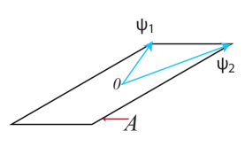
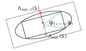
Figure 1: Left panel: the set $A=\{f_{\beta_{S}}:\|\beta_{S}\|_{1}=1\}$. Right panel: $\ell_{1}$- and $\ell_{2}$-eigenvalues.

The normalized compatibility constant $\phi(L,S)/\sqrt{s}$ is the minimal distance between the sets $A:=\{f_{\beta_{S}}:\ \|\beta_{S}\|_{1}=1\}$ and $B:=\{f_{\beta_{S^{c}}}:\ \|\beta_{S^{c}}\|_{1}\leq L\}$, that is,

$${\phi(L,S)\over\sqrt{s}}=\min\biggl{\{}\|a-b\|_{n}:\ a\in A,\ b\in B\biggr{\}}.$$

See Figure 2 for an impression of the situation. Observe that $A$ is the boundary of the convex hull of $\{+\psi_{j}\}_{j\in S}\cup\{-\psi_{j}\}_{j\in S}$, and $B$ is the convex hull of $\{+\psi_{j}\}_{j\in S^{c}}\cup\{-\psi_{j}\}_{j\in S^{c}}$ including its interior, blown up with a factor $L$ (typically, the $\{\psi_{j}\}_{j\in S^{c}}$ form a linearly dependent system in $\mathbb{R}^{n}$). Furthermore, since $\{0\}\in B$

$$\phi(L,S)\leq\Lambda_{{\rm min},1}(S).$$

This shows that when $\ell_{1}$-eigenvalues are small, the compatibility constant is necessarily also small. Small $\ell_{2}$-eigenvalues may have less of this effect.

Figure 2: The compatibility constant

6.2 Eigenvalues and entropy

We now let

$$\hat{\Sigma}=E\Omega^{2}E^{T}$$

be the spectral decomposition of the Gram matrix $\hat{\Sigma}$, $E$ being the matrix of eigenvectors, ($E^{T}E=EE^{T}=I$) and $\Omega^{2}={\rm diag}(\omega_{1}^{2},\cdots,\omega_{p}^{2})$ the matrix of ($\ell_{2}$-)eigenvalues. We assume they are in decreasing order: $\omega_{1}^{2}\geq\cdots\geq\omega_{p}^{2}$.

Lemma 6.1.

Suppose that for some strictly decreasing function $V$

$$\omega_{j+1}^{2}\leq V^{2}(j),\ j=1,\ldots,p.$$

Then for all $\delta>0$,

$$H(2\delta,\{f_{\beta}:\ \|\beta\|_{1}=1\},\|\cdot\|_{n})\leq V^{-1}(\delta)\log\biggl{(}{3\over\delta}\biggr{)}.$$

Example 6.1.

Suppose that for some positive constants $m$ and $C$

$$\omega_{j}\leq{C\over j^{m}},\ j=1,\ldots,p.$$

Then by Lemma 6.1,

$$H(2\delta,\{f_{\beta}:\ \|\beta\|_{1}=1\},\|\cdot\|_{n})\leq\biggl{(}{C\over\delta}\biggr{)}^{1\over m}\log\biggl{(}{3\over\delta}\biggr{)}.$$

For $\delta\geq 1/n$ (say) we therefore have

$$H(\delta,\{f_{\beta}:\ \|\beta\|_{1}=1\},\|\cdot\|_{n})\leq\biggl{(}{2C\over\delta}\biggr{)}^{1\over m}\log(6n).$$

When $m>1/2$, one can use a minor generalization of Corollary 5.2, where the entropy bound is only required for values of $\delta>1/n$. One then takes

$$\alpha={1\over 2m},\ A=(C_{m}^{2}\log(n))^{1\over 2\alpha},$$

where $C_{m}$ is a constant depending on $m$ and $C$. Then the value of $\lambda_{0}$ defined there becomes

$$\lambda_{0}={4K_{0}\over\sqrt{n}}\biggl{(}{C_{m}\sqrt{\log(n)}\over 2^{1-{1\over 2m}}-1}+t\biggr{)}$$

which is for fixed $m$ and $K_{0}$, and a fixed (large) $t$, of order $\sqrt{\log n/n}$.

6.3 Entropy based on coverings of $\{\psi_{j}\}$

We can consider $\{f_{\beta}:\|\beta\|_{1}=1\}$ as a subset of

$${\rm conv}(\{\pm\psi_{j}\}),$$

where $\{\pm\psi_{j}\}:=\{\psi_{j}\}\cup\{-\psi_{j}\}$, and ${\rm conv}(\{\pm\psi_{j}\})$ is its convex hull. Infact, if the $\{\psi_{j}\}$ form a linearly dependent system in $\mathbb{R}^{n}$, ${\cal F}$ is exactly equal to ${\rm conv}(\{\pm\psi_{j}\})$.

The paper [7] gives a bound for the entropy of a convex hull for the case where the $u$-covering number of the extreme points is a polynomial in $1/u$. This result can also be found in [9]. There is a redundant $\log$-term in these entropy bounds, see [1] and [15], but removing this $\log$-term may result in very large constants, depending on the dimension $W$ as given in Example 6.2 (see [3] for some explicit constants). This means that when the dimension $W$ of the extreme points is large (growing with $n$ say), the simple bound with $\log$-term we provide below in Lemma 6.2 may be better than the more involved ones.

We give a bound for the entropy of ${\cal F}$ by balancing the $u$-covering number of $\{\psi_{j}\}$ and the squared radius $u^{2}$. The result is as in [9], with only new element its extension to general covering numbers (i.e., not only polynomial ones). Lemma 6.2 and its proof can be found in [3].

Lemma 6.2.

Let

$$N(u):=N(u,\{\psi_{j}\},\|\cdot\|_{n}),\ u>0.$$

We have

$$H\biggl{(}\delta,\{f_{\beta}:\ \|\beta\|_{1}=1\},\|\cdot\|_{n}\biggr{)}$$

$$\leq\min_{0<u<1}6\left(N(u)+{6u^{2}\over\delta^{2}}\right)\log\biggl{(}2\biggl{(}{8+\delta\over\delta}\biggr{)}N(\delta)\biggr{)}.$$

Example 6.2.

In this example, we assume the $u$-covering numbers of $\{\psi_{j}\}$ are bounded by a polynomial in $u$. That is, we suppose that for some positive constants $W$ and $C$,

$$N(u,\{\psi_{j}\},\|\cdot\|_{n})\leq\biggl{(}{C\over u}\biggr{)}^{W},u>0.$$

The constant $W$ can be thought of as the dimension of $\{\psi_{j}\}$. By Lemma 6.2, we can choose

$$\alpha={W\over 2+W},\ A=(C_{W}^{2}\log(n))^{1\over 2\alpha},$$

and we get, as in Example 6.1,

$$\lambda_{0}={4K_{0}\over\sqrt{n}}\biggl{(}{C_{W}\sqrt{\log(n)}\over 2^{{2\over 2+W}}-1}+t\biggr{)}.$$

A refined analysis of the relation between compatibility constants, covering numbers and entropy is still to be carried out. We confine ourselves here to the following, rather trivial, observation (without proof).

Lemma 6.3.

Consider normalized design: $\|\psi_{j}\|_{n}=1$ $\forall\ j$. Let $\{\psi_{j_{1}},\ldots,\psi_{j_{N}}\}$ be a maximal $u$-packing set of $\{\psi_{j}\}$. Then for any $S\supset\{j_{1},\ldots,j_{N}\}$, $S\not=\{1,\ldots,p\}$, and any $L\geq 1$,

$$\phi^{2}(L,S)\leq su^{2}.$$

One may argue that as $u$-packing sets are approximations of the original design $\{\psi_{j}\}$ with fewer covariables, they are good candidates for the sparsity set $S_{1}$ used in Theorem 4.1. Lemma 6.3 however shows that such sparsity sets will have very small compatibility constants.

6.4 Decorrelation numbers

Decorrelation numbers are closely related to packing numbers. First, define the inner product

$$\rho(\phi,\tilde{\phi}):=\phi^{T}\tilde{\phi}/n.$$

Note that $\Sigma_{j,k}=\rho(\psi_{j},\psi_{k})$ and that in the case of standardized design (i.e. $\sum_{i=1}^{n}\psi_{j}(x_{i})=0$ and $\|\psi_{j}\|_{n}=1$ $\forall\ j$), the inner product $\rho(\psi_{j},\psi_{k})$ is for $j\not=k$ the (empirical) correlation between $\psi_{j}$ and $\psi_{k}$.

Definition For $\rho>0$, the $\rho$-decorrelation number $M(\rho)$ is the largest value of $M$ such that there exists $\{\phi_{1},\ldots,\phi_{M}\}\subset\{\pm\psi_{j}\}$ with $|\rho(\phi_{j},\phi_{k})|<\rho$ for all $j\not=k$.

Hence, if the $\rho$-decorrelation number is small, then there are many large correlations, i.e., then the design is highly correlated.

It is clear that when $\|\psi_{j}\|_{n}=\|\psi_{k}\|_{n}=1$, it holds that

$$\|\psi_{j}-\psi_{k}\|_{n}^{2}=2(1-\rho(\psi_{j},\psi_{k})).$$

In other words, small correlations correspond to covariables that are near to each other. This can be translated into covering number as shown in Lemma 6.4. Its proof is straightforward and omitted.

Lemma 6.4.

Consider normalized design: $\|\psi_{j}\|_{n}=1$ $\forall\ j$. For all $0<u<1$,

$$N(\sqrt{2}u,\{\pm\psi_{j}\},\|\cdot\|_{n})\leq M(1-u^{2}).$$

7 Conclusion

We have combined results for the prediction error of the Lasso with both compatibility conditions and entropy conditions. Small entropies of $\{f_{\beta}:\ \|\beta\|_{1}=1\}$ correspond to highly correlated design and possibly to small compatibility constants. Our analysis shows that small entropies allow for a smaller choice of the tuning parameter and possibly for a compensation of small compatibility constants. This means that the Lasso enjoys good prediction error properties, even in the case where the design is highly correlated.

8 Proofs

Proof of Lemma 4.1. We use that for positive $u$ and $v$ and for ${\rm p}\geq 1$, ${\rm q}\geq 1$, $1/{\rm p}+1/{\rm q}=1$, the conjugate inequality

$$uv\leq u^{\rm p}/{\rm p}+v^{\rm q}/{\rm q}$$

holds. Taking ${\rm p}=1/(1-\alpha)$ and replacing $u$ by $u^{1-\alpha}$ gives

$$u^{1-\alpha}v\leq{1-\alpha\over 2}u^{2}+{1+\alpha\over 2}v^{2\over 1+\alpha}.$$

With ${\rm p}=(1+\alpha)/(2\alpha)$, and replacing $u$ by $u^{2\alpha\over 1+\alpha}$, we get

$$u^{2\alpha\over 1+\alpha}v\leq{2\alpha\over 1+\alpha}u+{1-\alpha\over 1+\alpha}v^{1+\alpha\over 1-\alpha}.$$

Thus,

$$\lambda_{0}a^{1-\alpha}b^{\alpha}\leq{1-\alpha\over 2}a^{2}+{1+\alpha\over 2}\biggl{(}\lambda_{0}b^{\alpha}\biggr{)}^{2\over 1+\alpha}$$

$$\leq{a^{2}\over 2}+{1+\alpha\over 2}(\lambda b)^{2\alpha\over 1+\alpha}\biggl{(}{\lambda_{0}\over\lambda^{\alpha}}\biggl{)}^{2\over 1+\alpha}$$

$$\leq{a^{2}\over 2}+{1+\alpha\over 2}\left({2\alpha\over 1+\alpha}\lambda b+{1-\alpha\over 1+\alpha}\biggl{(}{\lambda_{0}\over\lambda^{\alpha}}\biggl{)}^{2\over 1-\alpha}\right)$$

$$\leq{a^{2}\over 2}+\lambda b+{1\over 2}\biggl{(}{\lambda_{0}\over\lambda^{\alpha}}\biggl{)}^{2\over 1-\alpha}.$$

$\sqcup\mkern-12.0mu\sqcap$

Proof of Theorem 4.1. Since

$$\|{\bf Y}-\hat{f}\|_{2}^{2}/n+\lambda\|\hat{\beta}\|_{1}\leq\|{\bf Y}-{\rm f}_{S}\|_{2}^{2}/n+\lambda\|b^{S}\|_{1},$$

we have the Basic Inequality

$$\|\hat{f}-f^{0}\|_{n}^{2}+\lambda\|\hat{\beta}\|_{1}\leq 2\epsilon^{T}(\hat{f}-{\rm f}_{S})/n+\lambda\|b^{S}\|_{1}+\|{\rm f}_{S}-f^{0}\|_{n}^{2}.$$

Hence, on ${\cal T}_{\alpha}$,

$$\|\hat{f}-f^{0}\|_{n}^{2}+\lambda\|\hat{\beta}\|_{1}\leq\lambda_{0}\|\hat{f}-{\rm f}_{S}\|_{n}^{1-\alpha}\|\hat{\beta}-b^{S}\|_{1}^{\alpha}/2+\lambda\|b^{S}\|_{1}+\|{\rm f}_{S}-f^{0}\|_{n}^{2}.$$

Apply Lemma 4.1 to find

$$\|\hat{f}-f^{0}\|_{n}^{2}+\lambda\|\hat{\beta}\|_{1}$$

$$\leq{1\over 4}\|\hat{f}-{\rm f}_{S}\|_{n}^{2}+{1\over 2}\lambda\|\hat{\beta}-b^{S}\|_{1}+{1\over 4}\biggl{(}{\lambda_{0}\over\lambda^{\alpha}}\biggr{)}^{2\over 1-\alpha}+\lambda\|b^{S}\|_{1}+\|{\rm f}_{S}-f^{0}\|_{n}^{2}.$$

$$\leq{1\over 2}\|\hat{f}-f^{0}\|_{n}^{2}+{1\over 2}\lambda\|\hat{\beta}-b^{S}\|_{1}+{1\over 4}\biggl{(}{\lambda_{0}\over\lambda^{\alpha}}\biggr{)}^{2\over 1-\alpha}+\lambda\|b^{S}\|_{1}+{3\over 2}\|{\rm f}_{S}-f^{0}\|_{n}^{2}.$$

Thus, we get on ${\cal T}_{\alpha}$,

$$\|\hat{f}-f^{0}\|_{n}^{2}+2\lambda\|\hat{\beta}\|_{1}\leq\lambda\|\hat{\beta}-b^{S}\|_{1}+2\lambda\|b^{S}\|_{1}+{1\over 2}\biggl{(}{\lambda_{0}\over\lambda^{\alpha}}\biggr{)}^{2\over 1-\alpha}+3\|{\rm f}_{S}-f^{0}\|_{n}^{2}.$$

Defining $S_{3}:=S^{c}$, we rewrite this to

$$\|\hat{f}-f^{0}\|_{n}^{2}+2\lambda\|\hat{\beta}_{S_{2}\cup S_{3}}\|_{1}$$

$$\leq\lambda\|\hat{\beta}_{S_{1}}-(b^{S})_{S_{1}}\|_{1}+\lambda\|\hat{\beta}_{S_{2}}-(b^{S})_{S_{2}}\|_{1}+\lambda\|\hat{\beta}_{S_{3}}\|_{1}+2\lambda\|(b^{S})_{S_{1}}\|_{1}-2\lambda\|\hat{\beta}_{S_{1}}\|_{1}$$

$$+2\lambda\|(b^{S})_{S_{2}}\|_{1}+{1\over 2}\biggl{(}{\lambda_{0}\over\lambda^{\alpha}}\biggr{)}^{2\over 1-\alpha}+3\|{\rm f}_{S}-f^{0}\|_{n}^{2}$$

$$\leq 3\lambda\|\hat{\beta}_{S_{1}}-(b^{S})_{S_{1}}\|_{1}+\lambda\|\hat{\beta}_{S_{2}\cup S_{3}}\|_{1}+3\lambda\|(b^{S})_{S_{2}}\|_{1}+{1\over 2}\biggl{(}{\lambda_{0}\over\lambda^{\alpha}}\biggr{)}^{2\over 1-\alpha}+3\|{\rm f}_{S}-f^{0}\|_{n}^{2}.$$

Moving the term $\lambda\|\hat{\beta}_{S_{2}\cup S_{3}}\|_{1}$ to the left hand side, and applying a triangle inequality, we obtain

$$\|\hat{f}-f^{0}\|_{n}^{2}+\lambda\|\hat{\beta}_{S_{2}\cup S_{3}}-(b^{S})_{S_{2}}\|_{1}$$

$$\leq\underbrace{3\lambda\|\hat{\beta}_{S_{1}}-(b^{S})_{S_{1}}\|_{1}}_{:=I}+\underbrace{4\lambda\|(b^{S})_{S_{2}}\|_{1}+{1\over 2}\biggl{(}{\lambda_{0}\over\lambda^{\alpha}}\biggr{)}^{2\over 1-\alpha}+3\|{\rm f}_{S}-f^{0}\|_{n}^{2}}_{:=II}.$$

Case i. If $I\geq II$, we arrive at

$$\|\hat{f}-f^{0}\|_{n}^{2}+\lambda\|\hat{\beta}_{S_{2}\cup S_{3}}-(b^{S})_{S_{2}}\|_{1}\leq 6\lambda\|\hat{\beta}_{S_{1}}-(b^{S})_{S_{1}}\|_{1}.$$

We first add add a term $\lambda\|\hat{\beta}_{S_{1}}-(b^{S})_{S_{1}}\|_{1}$ to the left and right hand side and then apply the compatibility condition to $\hat{\beta}-b^{S}$, to get

$$\|\hat{f}-f^{0}\|_{n}^{2}+\lambda\|\hat{\beta}-b^{S}\|_{1}\leq{7\lambda\sqrt{s_{1}}\over\phi(6,S_{1})}\|\hat{f}-{\rm f}_{S}\|_{n}$$

$$\leq{1\over 2}\|\hat{f}-f^{0}\|_{n}^{2}+{7\over 2}\|{\rm f}_{S}-f_{0}\|_{n}^{2}+{56\lambda^{2}s_{1}\over 2\phi^{2}(6,S_{1})}.$$

Here we used the decoupling device

$$2xy\leq bx^{2}+y^{2}/b\ \forall\ x,y\in R,\ b>0.$$

So then

$$\|\hat{f}-f^{0}\|_{n}^{2}+2\lambda\|\hat{\beta}-b^{S}\|_{1}\leq{56\lambda^{2}s_{1}\over\phi^{2}(6,S_{1})}+7\|{\rm f}_{S}-f^{0}\|_{n}^{2}.$$

Case ii. If $I<II$, we get

$$\|\hat{f}-f^{0}\|_{n}^{2}+\lambda\|\hat{\beta}_{S_{2}\cup S_{3}}-(b^{S})_{S_{2}}\|_{1}\leq 2II,$$

and hence

$$\|\hat{f}-f^{0}\|_{n}^{2}+\lambda\|\hat{\beta}-b^{S}\|_{1}\leq{7\over 3}II$$

$$={28\over 3}\lambda\|(b^{S})_{S_{2}}\|_{1}+{7\over 6}\biggl{(}{\lambda_{0}\over\lambda^{\alpha}}\biggr{)}^{2\over 1-\alpha}+7\|{\rm f}_{S}-f^{0}\|_{n}^{2}.$$

$\sqcup\mkern-12.0mu\sqcap$

Proof of Lemma 6.1. Let $\|\beta\|_{1}=1$. Then $\|\beta\|_{2}\leq 1$, and hence $\|E^{T}\beta\|_{2}\leq 1$. For $N\leq V^{-1}(\delta)$ it holds that $\omega_{N+1}\leq\delta$ and hence

$$\sum_{j=N+1}^{p}\omega_{j}^{2}(E^{T}\beta)_{j}^{2}\leq\omega_{N+1}^{2}\sum_{j=N+1}^{p}(E^{T}\beta)_{j}^{2}\leq\delta^{2}.$$

We now note that $\|\beta\|_{1}=1$ implies $\|f_{\beta}\|_{n}\leq 1$ and hence

$$\sum_{j=1}^{N}\omega_{j}^{2}(E^{T}\beta)_{j}^{2}\leq 1.$$

Lemma 14.27 in [3] states that a ball with radius $1$ in $N$-dimensional Euclidean space can be covered by $(3/\delta)^{N}$ balls with radius $\delta$ (see also Problem 2.1.6 in [15]). $\sqcup\mkern-12.0mu\sqcap$

References

- Ball and Pajor [1990] K. Ball and A. Pajor. The entropy of convex bodies with few extreme points. London Mathematical Society Lecture Note Series, 158:25–32, 1990.
- Bickel et al. [2009] P. Bickel, Y. Ritov, and A. Tsybakov. Simultaneous analysis of Lasso and Dantzig selector. Annals of Statistics, 37:1705–1732, 2009.
- Bühlmann and van de Geer [2011] P. Bühlmann and S. van de Geer. Statistics for High-Dimensional Data: Methods, Theory and Applications. Springer, 2011.
- Bunea et al. [2006] F. Bunea, A.B. Tsybakov, and M.H. Wegkamp. Aggregation and sparsity via -penalized least squares. In Proceedings of 19th Annual Conference on Learning Theory, COLT 2006. Lecture Notes in Artificial Intelligence 4005, pages 379–391, Heidelberg, 2006. Springer Verlag.
- Bunea et al. [2007a] F. Bunea, A.B. Tsybakov, and M.H. Wegkamp. Aggregation for Gaussian regression. Annals of Statistics, 35:1674–1697, 2007a.
- Bunea et al. [2007b] F. Bunea, A. Tsybakov, and M.H. Wegkamp. Sparsity oracle inequalities for the Lasso. Electronic Journal of Statistics, 1:169–194, 2007b.
- Dudley [1987] R.M. Dudley. Universal Donsker classes and metric entropy. Annals of Probability, 15:1306–1326, 1987.
- Koltchinskii [2009] V. Koltchinskii. Sparsity in penalized empirical risk minimization. Annales de l’Institut Henri Poincaré, Probabilités et Statistiques, 45:7–57, 2009.
- Pollard [1990] D. Pollard. Empirical Processes: Theory and Applications. IMS Lecture Notes, 1990.
- van de Geer [2007a] S. van de Geer. The deterministic Lasso. The JSM Proceedings, 2007a.
- van de Geer [2008] S. van de Geer. High-dimensional generalized linear models and the Lasso. Annals of Statistics, 36:614–645, 2008.
- van de Geer [2007b] S. van de Geer. On non-asymptotic bounds for estimation in generalized linear models with highly correlated design. In Asymptotics: Particles, Processes and Inverse Problems (E.A. Cator, G. Jongbloed, C. Kraaikamp, H.P. Lopuhaä, J.A. Wellner eds.), volume 55, pages 121–134. IMS Lecture Notes Monograph Series, 2007b.
- van de Geer and Bühlmann [2009] S. van de Geer and P. Bühlmann. On the conditions used to prove oracle results for the Lasso. Electronic Journal of Statistics, pages 1360–1392, 2009.
- van de Geer [2000] S. A. van de Geer. Empirical Processes in M-Estimation. Cambridge, 2000.
- van der Vaart and Wellner [1996] A. W. van der Vaart and J. A. Wellner. Weak Convergence and Empirical Processes. Springer Series in Statistics. Springer-Verlag, New York, 1996. ISBN 0-387-94640-3.