Unstructured Human Activity Detection from RGBD Images

Abstract

Being able to detect and recognize human activities is essential for several applications, including personal assistive robotics. In this paper, we perform detection and recognition of unstructured human activity in unstructured environments. We use a RGBD sensor (Microsoft Kinect) as the input sensor, and compute a set of features based on human pose and motion, as well as based on image and point-cloud information. Our algorithm is based on a hierarchical maximum entropy Markov model (MEMM), which considers a person’s activity as composed of a set of sub-activities. We infer the two-layered graph structure using a dynamic programming approach. We test our algorithm on detecting and recognizing twelve different activities performed by four people in different environments, such as a kitchen, a living room, an office, etc., and achieve good performance even when the person was not seen before in the training set.

I Introduction

Being able to automatically infer the activity that a person is performing is essential in many applications, such as in personal assistive robotics. For example, if a robot could watch and keep track of how often a person drinks water, it could prevent the dehydration of elderly by reminding them. True daily activities do not happen in structured environments (e.g., with closely controlled background), but in uncontrolled and cluttered households and offices. Due to its unstructured and often visually confusing nature, detection of daily activities becomes a much more difficult task. In addition, each person has his or her own habits and mannerisms in carrying out tasks, and these variations in speed and style create additional difficulties in trying to detect and recognize activities. In this work, we are interested in reliably detecting daily activities that a person performs in a home or office, such as cooking, drinking water, brushing teeth, talking on the phone, and so on.

Most previous work on activity classification has focused on using 2D video (e.g., [26, 10]) or RFID sensors placed on humans and objects (e.g., [41]). The use of 2D videos leads to relatively low accuracy (e.g., 78.5% in [19]) even when there is no clutter. The use of RFID tags is generally too intrusive because it requires a placement of RFID tags on the people.

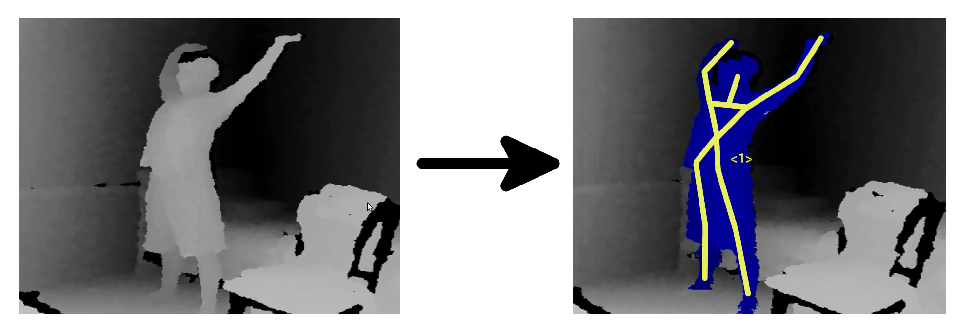
Figure 1: The RGBD data from the Kinect sensor is used to generate an articulated skeleton model. This skeleton is used along with the raw image and depths for estimating the human activity.

In this work, we perform activity detection and recognition using an inexpensive RGBD sensor (Microsoft Kinect). Human activities, despite their unstructured nature, tend to have a natural hierarchical structure; for instance, drinking water involves a three-step process of bringing a glass to one’s mouth, tilting the glass and head to drink, and putting the glass down again. We can capture this hierarchical nature using a hierarchical probabilistic graphical model—specifically, a two-layered maximum entropy Markov model (MEMM). Even with this structured model in place, different people perform tasks at different rates, and any single graphical model will likely fail to capture this variation. To overcome this problem, we present a method of on-the-fly graph structure selection that can automatically adapt to variations in task speeds and style. Finally, we need features that can capture meaningful characteristics of the person. We accomplish this by using the PrimeSense skeleton tracking system [27] in combination with specially placed Histogram of Oriented Gradient [4] computer vision features. This approach enables us to achieve reliable performance in detection and recognition of common activities performed in typical cluttered human environments.

We evaluated our method on twelve different activities (see Figure 3) performed by four different people in five different environments: kitchen, office, bathroom, living room and bedroom. Our results show a precision/recall of 84.7%/83.2% in detecting the correct activity when the person was seen before in the training set and 67.9%/55.5% when the person was not seen before. We have also made the dataset and code available open-source at: http://pr.cs.cornell.edu/humanactivities

II Related Work

There is a large body of previous work on human activity recognition. One common approach is to use space-time features to model points of interest in video [15, 6]. Several authors have supplemented these techniques by adding more information to these features [11, 40, 41, 19, 25, 30]. However, this approach is only capable of classifying, rather than detecting, activities. Other approaches include filtering techniques [29] and sampling of video patches [1]. Hierarchical techniques for activity recognition have been used as well, but these typically focus on neurologically-inspired visual cortex-type models [9, 32, 23, 28]. Often, these authors adhere faithfully to the models of the visual cortex, using motion-direction sensitive “cells” such as Gabor filters in the first layer [11, 26].

Another class of techniques used for activity recognition is that of the hidden Markov model (HMM). Early work by Brand et al. [2] utilized coupled HMMs to recognize two-handed activities. Weinland et al. [38] used an HMM together with a 3D occupancy grid to model human actions. Martinez-Contreras et al. [21] utilized motion templates together with HMMs to recognize human activities. As well as generative models like HMM, Lan et al. [14] employed a discriminative model which was aided by interaction analysis between people. Sminchisescu et al. [33] used conditional random fields (CRF) and maximum-entropy Markov models, arguing that these models overcome some of the limitations presented by HMMs. Notably, HMMs create long-term dependencies between observations and tries to model observations, which are already fixed at runtime. On the other hand, MEMM and CRF are able to avoid such dependencies and enables longer interaction among observations. However, the use of 2D videos leads to relatively low accuracies.

Other authors have worked on hierarchical dynamic Bayesian networks. Early work by Wilson and Bobick [39] extended HMM to parametric HMM for recognizing pointing gestures. Fine et al. [8] introduced hierarchical HMM, which was later extended by Bui et al. [3] to a general structure in which each child can have multiple parents. Truyen et al. [36] then developed a hierarchical semi-Markov CRF that could be used in partially observable settings. Liao et al. [18] applied hierarchical CRFs to activity recognition but their model requires many GPS traces and is only capable of off-line classification. Wang et al. [37] proposed Dual Hierarchical Dirichlet Processes for surveillance of the large area. Among several others, the hierarchical HMM is the closest model of these to ours, but does not capture the idea that a single state may connect to different parents only for specified periods of time, as our model does. As a result, none of these models fit our problem of online detection of human activities in uncontrolled and cluttered environment. Since MEMM enables longer interaction among observations unlike HMM [33], the hierarchical MEMM allows us to take new observations and utilize dynamic programming to consider them in an online setting.

Various robotic systems have used activity recognition before. Theodoridis et al. [35] used activity recognition in robotic systems to discern aggressive activities in humans. Li et al. [17] discuss the importance of non-verbal communication between human and robot and developed a method to recognize simple activities that are nondeterministic in nature, while other works have focused on developing robots that utilizes activity recognition to imitate human activities [5, 20]. However, we are more interested here in assistive robots. Assistive robots are robots that assist humans in some task. Several types of assistive robots exist, including socially assistive robots that interact with another person in a non-contact manner, and physically assistive robots, which can physically help people [7, 34, 24, 16, 12, 13].

III Our Approach

We use a supervised learning approach in which we collected ground-truth labeled data for training our model. Our input is RGBD images from a Kinect sensor, from which we extract certain features that are fed as input to our learning algorithm. We train a two-layered maximum-entropy Markov model which will capture different properties of human activities, including their hierarchical nature and the transitions between sub-activities over time.

III-A Features

We can recognize a person’s activity by looking at his current pose and movement over time, as captured by a set of features. The input sensor for our robot is a RGBD camera (Kinect) that gives us an RGB image as well as depths at each pixel. In order to compute the human pose features, we describe a person by a rigid skeleton that can move at fifteen joints (see Figure 1). We extract this skeleton using a tracking system provided by PrimeSense [27]. The skeleton is described by the length of the links and the joint angles. Specifically, we have the three-dimensional Euclidean coordinates of each joint and the orientation matrix of each joint with respect to the sensor. We compute features from this data as follows.

Body pose features. The joint orientation is obtained with respect to the sensor. However, we are interested in true pose, which is invariant of sensor location. Therefore, we transform each joint’s rotation matrix so that the rotation is given with respect to the person’s torso. For 10 joints, we convert each rotation matrix to half-space quaternions in order to more compactly represent the joint’s orientation. (A more compact representation would be to use Euler angles, but they suffer from representation problem called gimbal lock [31].) Along with these joint orientations, we would like to know whether person is standing or sitting, and whether or not person is leaning over. Such information is observed from the position of each foot with respect to the torso ($3*2$) by using the head and hip joints to compute the angle of the upper body against vertical. We have $10*4+3*2+1=47$ features for the body pose.

Hand Position. Hands play an especially important role in carrying out many activities, so information about what hands are doing can be quite powerful. In particular, we want to capture information such as “the left hand is near the stomach” or “the right hand is near the right ear.” To do this, we compute the position of the hands with respect to the torso, and with the respect to the head in the local coordinate frame. Though we capture the motion information as described next, in order to emphasize hand movement, we also observe hand position over last 6 frames and record the highest and lowest vertical hand position. We have $2*(6+2)=16$ features for this.

Motion Information. Motion information is also important for classifying a person’s activities. We select nine frames spread out over the last three seconds, spaced as follows: $\{-5,-9,-14,-20,-27,-35,-44,-54,-65\}$, where the numbers refer to the frames chosen. Then, we compute the joint rotations that have occurred between each of these frames and the current frame, represented as half-space quaternions (for the 11 joints with orientation information). This gives. $9*11*4=396$ features. We refer to body pose, hand and motion features as “skeletal features”.

Image and point-cloud features. Much useful information can be derived directly from the raw image and point cloud as well. We use the Histogram of Oriented Gradients (HOG) feature descriptors [4], which gives 32 features that count how often certain gradient orientations are seen in specified bounding boxes of an image. Although this computation is typically performed on RGB or grayscale images, we can also view the depth map as a grayscale image and compute the HOG features on that. We have two HOG settings that we use. In the “simple HOG” setting, we find the bounding box of the person in the image, and compute RGB and depth HOG features for that bounding box, for a total of 64 features. In the “skeletal HOG” setting, we use the extracted skeleton model to find the bounding boxes for the person’s head, torso, left arm, and right arm, and we compute the RGB and depth HOG features for each of these four bounding boxes, for a total of 256 features. In this paper’s primary result, we use the “skeletal HOG” setting.

III-B Model Formulation

Human activity is complex and dynamic, and therefore our learning algorithm should model different nuances in human activities, such as the following.

First, an activity comprises a series of sub-activities. For example, the activity “brushing teeth” consists of sub-activities such as “squeezing toothpaste,” “bringing toothbrush up to face,” “brushing,” and so forth. Therefore for each activity (represented by $z\in Z$), we will model sub-activities (represented by $y\in Y$). We will train a hierarchical Markov model where the sub-activities $y$ are represented by a layer of hidden variables (see Figure 2).

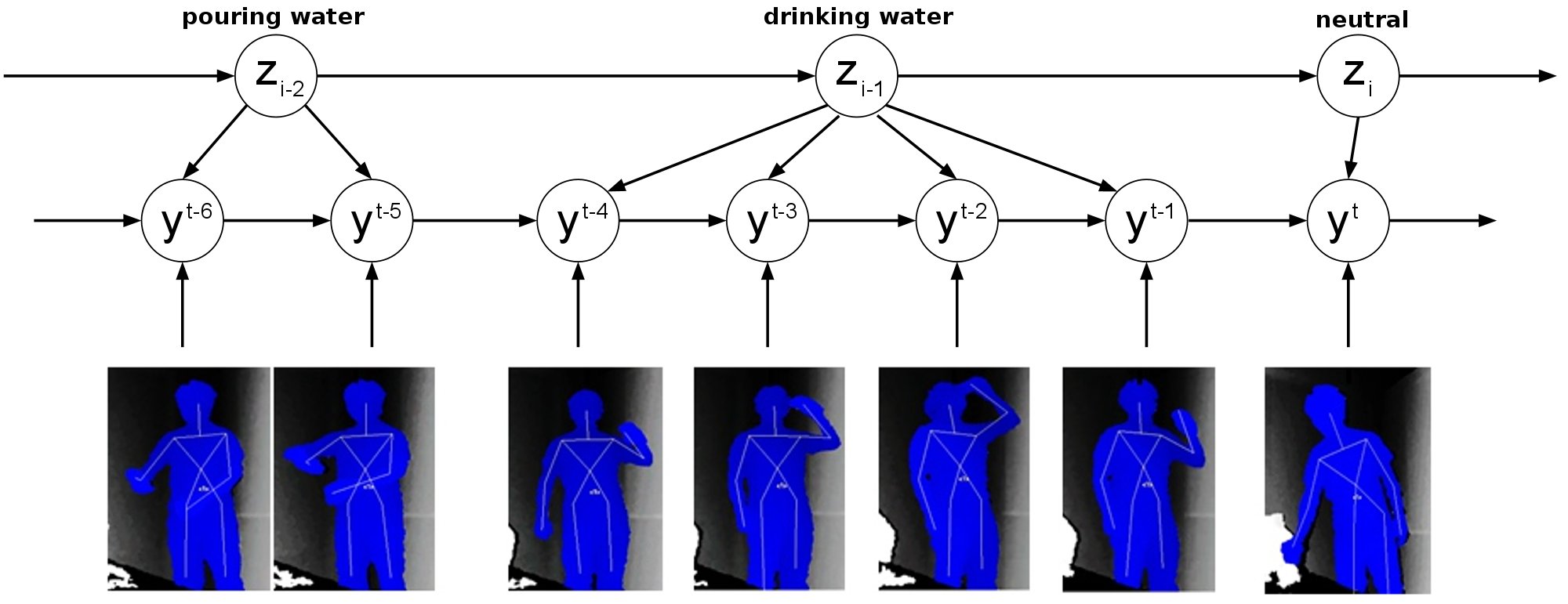
Figure 2: Our two-layered MEMM model.

For each activity, different subjects perform the sub-activities for different periods of time. It is not clear how to associate the sub-activities to the activities. This implies that the graph structure of the model cannot be fixed in advance. We therefore determine the connectivity between the $z$ and the $y$ layers in the model during inference.

Model. Our model is based on a maximum-entropy Markov model (MEMM) [22]. However, in order to incorporate the hierarchical nature of activities, we use a two-layered hierarchical structure, as shown in Figure 2.

In our model, let $x^{t}$ denote the features extracted from the articulated skeleton model at time frame $t$. Every frame is connected to high-level activities through the mid-level sub-activities. Since high-level activities do not change every frame, we do not index them by time. Rather, we simply write $z_{i}$ to denote the $i^{th}$ high-level activity. Activity $i$ occurs from time $t_{i-1}+1$ to time $t_{i}$. Then $\{y^{t_{i-1}+1},...,y^{t_{i}}\}$ is the set of sub-activities connected to activity $z_{i}$.

III-C MEMM with Hierarchical Structure

As shown in Figure 2, each node $z_{i}$ in the top layer is connected to several consecutive nodes in the middle layer $\{y^{t_{i-1}+1},...,y^{t_{i}}\}$, capturing the intuition that a single activity consists of a number of consecutive sub-activities.

For the sub-activity at each frame $y^{t}$, we do not know a priori to which activity $z_{i}$ it should connect at the top layer. Therefore, our algorithm must decide when to connect a middle-layer node $y^{t}$ to top-layer node $z_{i}$ and when to connect it to next top-layer node $z_{i+1}$. We show in the next section how selection of graph structure can be done through dynamic programming. Given the graph structure, our goal is to infer the $z_{i}$ that best explains the data. We do this by modeling the joint distribution $P(z_{i},y^{t_{i-1}+1}\cdots y^{t_{i}}|O_{i},z_{i-1})$ where $O_{i}=x^{t_{i-1}+1},...,x^{t_{i}}$, and for each $z_{i}$, we find the set of $y^{t}$’s that maximize the joint probability. Finally, we choose the $z_{i}$ that has the highest joint probability distribution.

Learning Model. We use a Gaussian mixture model to cluster the original training data into separate clusters, and consider each cluster as a sub-activity, rather than manually labeling sub-activities for each frame. We constrain the model to create five clusters for each activity, and then combine all the clusters for a certain location’s activities into a single set of location specific clusters. In addition, we also generate a few clusters from the negative examples, so that our algorithm becomes robust to not detecting random activities. Specifically, for each classifier and for each location, we create a single cluster from each of the activities that do not occur in that location.

Our model consists of the following three terms:

• $P(y^{t}|x^{t})$: This term models the dependence of the sub-activity label $y^{t}$ on the features $x^{t}$. We model this using the Gaussian mixture model we have built. The parameters of the model are estimated from the labeled training data using maximum-likelihood.

• $P(y^{t_{i}-m}|y^{t_{i}-m-1},z_{i})$ (where $m\in\{0,...,(t_{i}-t_{i-1}-1)\}$). A sequence of sub-activities describes the activities. For example, we can say the sequence “squeezing toothpaste,” “bringing toothbrush up to face,” “actual brushing,” and “putting toothbrush down” describes the activity “brushing teeth.” If we only observe “bringing toothbrush up to face” and “putting toothbrush down,” we would not refer to it as “brushing teeth.” Unless the activity goes through a specific set of sub-activities in nearly the same sequence, it should probably not be classified as the activity. For all the activities except neutral, the table is built from observing the transition of posterior probability for soft cluster of Gaussian mixture model at each frame.

  However, it is not so straightforward to build $P(y^{t_{i}-m}|y^{t_{i}-m-1},z_{i})$ when $z_{i}$ is neutral. When a sub-activity sequence such as “bringing toothbrush to face” and “putting toothbrush down” occurs, it does not correspond to any known activity and so is likely to be neutral. It is not possible to collect data of all sub-activity sequences that do not occur in our list of activities, so we rely on the sequences observed from non-neutral activities. If $N$ denotes neutral activity, then $P(y^{t_{i}-m}|y^{t_{i}-m-1},z_{i}=N)\propto 1-\sum\limits_{z_{i}\neq N}P(y^{t_{i}-m}|y^{t_{i}-m-1},z_{i}).$

• $P(z_{i}|z_{i-1})$. The activities evolve over time. For example, one activity may be more likely to follow another, and there are brief moments of neutral activity between two non-neutral activities. Thus, we can make a better estimate of the activity at the current time if we also use the estimate of the activity at previous time-step. Unlike other terms, due to difficulty of obtaining rich data set for maximum likelihood estimation, $P(z_{i}|z_{i-1})$ is set manually to capture these intuitions.

Inference. Consider the two-layer MEMM depicted in Figure 2. Let a single $z_{i}$ activity node along with all the $y^{t}$ sub-activity nodes connected directly to it and the corresponding $x^{t}$ feature inputs be called a substructure of the MEMM graph. Given an observation sequence $O_{i}=x^{t_{i-1}+1},...,x^{t_{i}}$ and a previous activity $z_{i-1}$, we wish to compute the joint probability $P(z_{i},y^{t_{i-1}+1}\dotsb y^{t_{i}}|O_{i},z_{i-1})$:

$$P(z_{i} ,y^{t_{i-1}+1}\dotsb y^{t_{i}}|O_{i},z_{i-1})$$

$$= P(z_{i}|O_{i},z_{i-1})P(y^{t_{i-1}+1}\dotsb y^{t_{i}}|z_{i},O_{i},z_{i-1})$$

$$= P(z_{i}|z_{i-1})\cdot{\displaystyle\prod^{t_{i}}_{t=t_{i-1}+2}P(y^{t}|y^{t-1},z_{i},x^{t})}$$

$$\cdot\sum\limits_{y^{t_{i-1}}}P(y^{t_{i-1}+1}|y^{t_{i-1}},z_{i},x^{t_{i-1}+1})P(y^{t_{i-1}})$$

We have all of these terms except $P(y^{t}|y^{t-1},z_{i},x^{t})$ and $P(y^{t_{i-1}+1}|y^{t_{i-1}},z_{i},x^{t_{i-1}+1})$. Both terms can be derived as

$$P(y^{t}|y^{t-1},z_{i},x^{t})={P(y^{t-1},z_{i},x^{t}|y^{t})P(y^{t})\over P(y^{t-1},z_{i},x^{t})}$$

We make a naive Bayes conditional independence assumption that $$y^{t-1} z_{i} x^{t} y^{t}$$ and are independent from given . Using this assumption, we get:

$$P(y^{t}|y^{t-1},z_{i},x^{t})={P(y^{t}|y^{t-1},z_{i})P(y^{t}|x^{t})\over P(y^{t})}$$

We have fully derived $P(z_{i},y^{t_{i-1}+1}\dotsb y^{t_{i}}|O_{i},z_{i-1})$:

$$P( z_{i},y^{t_{i-1}+1}\dotsb y^{t_{i}}|O_{i},z_{i-1})=P(z_{i}|z_{i-1})$$

$$\cdot\sum\limits_{y^{t_{i-1}}}{P(y^{t_{i-1}+1}|y^{t_{i-1}},z_{i})P(y^{t_{i-1}+1}|x^{t_{i-1}+1})\over P(y^{t_{i-1}+1})}P(y^{t_{i-1}})$$

$$\cdot\displaystyle\prod^{t_{i}}_{t=t_{i-1}+2}{{P(y^{t}|y^{t-1},z_{i})P(y^{t}|x^{t})\over P(y^{t})}}$$

Note that this formula can be factorized into two terms where one of them only contains two variables.

$$P(z_{i},y^{t_{i-1}+1}\dotsb y^{t_{i}}|O_{i},z_{i-1})=\mathcal{A}\cdot\displaystyle\prod^{t_{i}}_{t=t_{i-1}+2}\mathcal{B}(y^{t-1},y^{t})$$

Because the formula has factored into terms containing only two variables each, this equation can be easily and efficiently optimized. We simply optimize each factor individually, and we obtain:

$$\max P(z_{i} ,y^{t_{i-1}+1}\dotsb y^{t_{i}}|O_{i},z_{i-1})=\max\limits_{y^{t_{i-1}+1}}\mathcal{A}$$

$$\cdot\max\limits_{y^{t_{i-1}+2}}\mathcal{B}(y^{t_{i-1}+1},y^{t_{i-1}+2})\dotsb\max\limits_{y^{t_{i}}}\mathcal{B}(y^{t_{i}-1},y^{t_{i}})$$

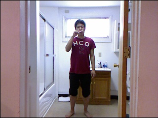
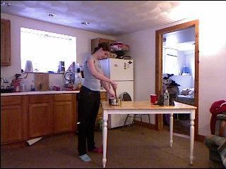
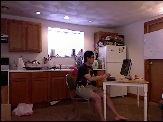
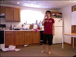
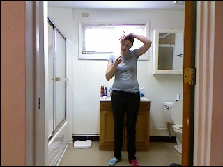
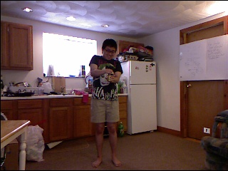
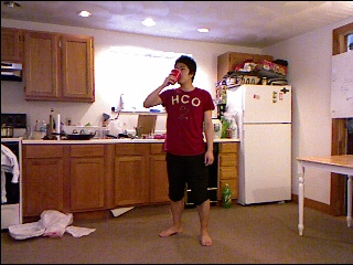
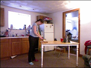
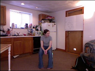
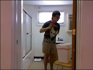
Figure 3: Samples from our dataset. Row-wise, from left: brushing teeth, cooking (stirring), writing on whiteboard, working on computer, talking on phone, wearing contact lenses, relaxing on a chair, opening a pill container, drinking water, cooking (chopping), talking on a chair, and rinsing mouth with water.

III-D Graph Structure Selection

Now that we can find the set of $y^{t}$’s that maximize the joint probability $P(z_{i},y^{t_{i-1}+1}\dotsb y^{t_{i}}|O_{i},z_{i-1})$, the probability of an activity $z_{i}$ being associated with the $i^{th}$ substructure and the previous activity, we wish to use that to compute the probability of $z_{i}$ given all observations up to this point. However, to do this, we must solve the following problem: for each observation $y^{t}$, we must decide to which high-level activity $z_{i}$ it should be connected (see Figure 2). For example, consider the last $y$ node associated with the “drinking water” activity in Figure 2. It’s not entirely clear if that node really should connect to the “drinking water” activity, or if it should connect to the following “neutral” activity. Deciding with which activity node to associate each $y$ node is the problem of hierarchical MEMM graph structure selection.

Unfortunately, we cannot simply try all possible graph structures. To see why, suppose we have a graph structure at time $t-1$ with a final high-level node $z_{i}$, and then are given a new node $y^{t}$. This node has two “choices”: it can either connect to $z_{i}$, or it can create a new high-level node $z_{i+1}$ and connect to that one. Because every node $y^{t}$ has this same choice, if we see a total of $n$ mid-level nodes, then there are $2^{n}$ possible graph structures.

We present an efficient method to find the optimal graph structure using dynamic programming. The method works, in brief, as follows. When given a new frame for classification, we try to find the point in time at which the current high-level activity started. So we pick a time $t^{\prime}$, and say that every frame after $t^{\prime}$ belongs to the current high-level activity. We have already computed the optimal graph structure for the first $t^{\prime}$ time frames, so putting these two subgraphs together give us a possible graph structure. We can then use this graph to compute the probability that the current activity is $z$. By trying all possible times $t^{\prime}<t$, we can find the graph structure that gives us the highest probability, and we select that as our graph structure at time $t$.

The Method of Graph Structure Selection. Now we describe the method in detail. Suppose we are at some time $t$; we wish to select the optimal graph structure given everything we have seen so far. We will define the graph structure inductively based on graph structures that were chosen at previous points in time. Let $G_{t^{\prime}}$ represent the graph structure that was chosen at some time $t^{\prime}<t$. Note that, as a base case, $G_{0}$ is always the empty graph.

For every $t^{\prime}<t$, define a candidate graph structure $\tilde{G}_{t}^{t^{\prime}}$ consisting of $G_{t^{\prime}}$ (the graph structure capturing the first $t^{\prime}$ timeframes), followed by a single substructure from time $t^{\prime}+1$ to time $t$ connected to a single high-level node $z_{i}$. Note that this candidate graph structure sets $t_{i-1}=t^{\prime}$ and $t_{i}=t$. Given the set of candidate structures $\{\tilde{G}_{t}^{t^{\prime}}|1\leq t^{\prime}<t\}$, the plan is to find the graph structure and high-level activity $z_{i}\in Z$ to maximize the likelihood given the set of observations so far.

Let $O$ be the set of all observations so far. Then $P(z_{i}|O;\tilde{G}_{t}^{t^{\prime}})$ is the probability that the most recent high-level node $i$ is activity $z_{i}\in Z$, given all observations so far and parameterized by the graph structure $\tilde{G}_{t}^{t^{\prime}}$. We initially set $P(z_{0}|O;G_{0})$ to a uniform distribution. Then, through dynamic programming, we have $P(z_{i-1}|O;G_{t^{\prime}})$ for all $t^{\prime}<t$ and all $z\in Z$ (details below). Suppose that, at time $t$, we choose the graph structure $\tilde{G}_{t}^{t^{\prime}}$ for a given $t^{\prime}<t$. Then the probability that the most recent node $i$ is activity $z_{i}$ is given by

$$P(z_{i}|O;\tilde{G}_{t}^{t^{\prime}})= \sum_{z_{i-1}}P(z_{i},z_{i-1}|O;\tilde{G}_{t}^{t^{\prime}})$$

$$= \sum_{z_{i-1}}P(z_{i-1}|O;\tilde{G}_{t}^{t^{\prime}})P(z_{i}|O,z_{i-1};\tilde{G}_{t}^{t^{\prime}})$$

$$= \sum_{z_{i-1}}P(z_{i-1}|O;G_{t^{\prime}})P(z_{i}|O_{i},z_{i-1})$$ (1)

The two factors inside the summation are terms that we know, the former due to dynamic programming, and the latter estimated by finding maximum of $P(z_{i},y^{t_{i-1}+1}\dotsb y^{t_{i}}|O_{i},z_{i-1})$, described in the previous section.

Thus, to find the optimal probability of having node $i$ be a specific activity $z_{i}$, we simply compute

$$P(z_{i}|O;G_{t})=\max_{t^{\prime}<t}P(z_{i}|O;\tilde{G}_{t}^{t^{\prime}})$$

We store $P(z_{i}|O;G_{t})\;\forall\,z_{i}$ for dynamic programming purposes (Equation III-D). Then, to make a prediction of an activity at time $t$, we compute

$$\mbox{activity}_{t}=\arg\max_{z_{i}}P(z_{i}|O)=\arg\max_{z_{i}}\max_{t^{\prime}<t}P(z_{i}|O;\tilde{G}_{t}^{t^{\prime}})$$

Optimality. We show that this algorithm is optimal by induction on the time $t$. Suppose we know the optimal graph structure for every time $t^{\prime}<t$. This is certainly true at time $t=1$, as the optimal graph structure at time $t=0$ is the empty graph. The optimal graph structure at time $t$ involves a final high-level node $z_{i}$ that is connected to $1\leq k\leq t$ mid-level nodes.

Suppose the optimal structure at time $t$ has the high-level node connected to $k=t-t^{\prime}$ mid-level nodes. Then what graph structure do we use for the first $t^{\prime}$ nodes? By the induction hypothesis, we know the optimal graph structure $G_{t^{\prime}}$ for the first $t^{\prime}$ nodes. That is, $G_{t^{\prime}}$ is the graph structure that maximizes the probability $P(z_{i-1}|O)$. Because $z_{i}$ is conditionally independent of any high-level node before $z_{i-1}$, the graph structure before $z_{i-1}$ does not affect $z_{i}$. Similarly, the graph structure before $z_{i-1}$ obviously does not depend on the graph structure after $z_{i-1}$. Therefore, the optimal graph structure at time $t$ is $\tilde{G}_{t}^{t^{\prime}}$, the concatenation of $G_{t^{\prime}}$ to a single substructure of $t-t^{\prime}$ nodes.

We do not know what the correct time $0\leq t^{\prime}<t$ is, but because we try all, we are guaranteed to find the optimal $t^{\prime}$, and therefore the optimal graph structure.

Complexity. Let n and m be the number of activities and sub-activities, respectively, and let t be the time. Space complexity for the dynamic programming algorithm is $O(n\cdot t)$ since we store 1-d array of size t for each activity. At each timeframe, we must compute the optimal graph structure. By setting a maximum substructure size of $T\ll t$, dynamic programming requires $n$ activities to be checked for each of $T$ possible sizes. Each check requires a computation of $P(z_{i},y^{t_{i-1}+1}\dotsb y^{t_{i}}|O_{i},z_{i-1})$, which takes $O(m\cdot T)$ time. Thus, each timeframe requires $O(n\cdot m\cdot T^{2})$ computation time. We do this computation for each of $t$ timeframes, for an overall time complexity of $O(n\cdot m\cdot T^{2}\cdot t)$.

TABLE I: Results of naive classifier, one-level MEMM model, and our full model in each location. The table shows precision and recall scores for all of our models. Note that the test dataset contains random movements (in addition to the activities considered), ranging from a person standing still to walking around while waving his or her hands. RGB(D) HOG refers to “simple HOG”.

		“New Person”										“Have Seen”
		Naive		One-layer		Full Model						Naive		One-layer		Full Model
		Classifier		MEMM		RGB HOG		RGBD HOG		Skel.+Skel HOG		Classifier		MEMM		Skel.+Skel HOG
Location	Activity	Prec	Rec	Prec	Rec	Prec	Rec	Prec	Rec	Prec	Rec	Prec	Rec	Prec	Rec	Prec	Rec
bathroom	rinsing mouth	77.7	49.3	71.8	63.2	42.2	73.3	49.1	97.3	51.1	51.4	73.3	49.7	70.7	53.1	61.4	70.9
	brushing teeth	64.5	20.5	83.3	57.7	50.7	30.8	73.4	16.6	88.5	55.3	81.5	65.1	81.5	75.6	96.7	77.1
	wearing contact lens	82.0	89.7	81.5	89.7	44.2	40.6	52.5	59.5	78.6	88.3	87.8	71.9	87.8	71.9	79.2	94.7
	Average	74.7	53.1	78.9	70.2	45.7	48.2	58.3	57.8	72.7	65.0	80.9	62.2	80.0	66.9	79.1	80.9
bedroom	talking on the phone	82.0	32.6	82.0	32.6	0.0	0.0	15.6	8.8	63.2	48.3	70.2	67.2	70.2	69.0	88.7	90.8
	drinking water	19.2	12.1	19.1	12.1	0.0	0.0	3.0	0.1	70.0	71.7	64.1	31.6	64.1	39.6	83.3	81.7
	opening pill container	95.6	65.9	95.6	65.9	60.6	34.8	33.8	36.5	95.0	57.4	48.7	52.3	48.7	54.8	93.3	77.4
	Average	65.6	36.9	65.6	36.9	20.2	11.6	17.4	15.2	76.1	59.2	61.0	50.4	61.0	54.5	88.4	83.3
kitchen	cooking (chopping)	33.3	56.9	33.2	57.4	56.1	90.0	59.9	74.2	45.6	43.3	78.9	28.9	78.9	29.0	70.3	85.7
	cooking (stirring)	44.2	29.3	45.6	31.4	58.0	4.0	94.5	11.1	24.8	17.7	44.6	45.8	44.6	45.8	74.3	47.3
	drinking water	72.5	21.3	71.6	23.9	0.0	0.0	91.8	23.9	95.4	75.3	52.2	51.5	52.2	52.4	88.8	86.8
	opening pill container	76.9	6.2	75.8	6.2	83.6	33.5	54.1	35.0	91.9	55.2	17.9	62.4	17.9	62.4	91.0	77.4
	Average	56.8	28.4	56.6	29.7	49.4	31.9	75.1	36.1	64.4	47.9	48.4	47.2	48.4	47.4	81.1	74.3
	talking on the phone	69.7	0.9	83.3	25.0	0.0	0.0	31.0	11.8	51.5	48.5	34.1	67.7	34.1	67.7	88.8	90.6
living	drinking water	57.1	53.1	52.8	55.8	0.0	0.0	1.2	0.0	54.3	69.3	80.2	48.7	71.0	53.8	80.2	82.6
room	talking on couch	71.5	35.4	57.4	91.3	42.7	59.4	53.2	63.2	73.2	43.7	91.4	50.7	91.4	50.7	98.8	94.7
	relaxing on couch	97.2	76.4	95.8	78.6	0.0	0.0	100.0	21.5	31.3	21.1	95.7	96.5	95.7	96.5	86.8	82.7
	Average	73.9	41.5	72.3	62.7	10.7	14.9	46.4	24.1	52.6	45.7	75.4	65.9	73.1	67.2	88.7	87.7
office	talking on the phone	60.5	31.0	60.6	31.5	17.5	6.7	2.7	0.6	69.4	48.2	80.4	52.2	80.4	52.2	87.6	92.0
	writing on whiteboard	47.1	73.3	45.2	74.1	41.2	25.1	94.0	97.0	75.5	81.3	42.5	59.3	42.5	59.3	85.5	91.9
	drinking water	41.1	12.4	51.2	23.2	0.0	0.0	0.0	0.0	67.1	68.8	53.4	36.7	53.4	36.7	82.3	81.5
	working on computer	93.5	76.8	93.5	76.8	100.0	11.9	100.0	29.0	83.4	40.7	89.2	69.3	89.2	69.3	89.5	93.8
	Average	60.5	48.4	62.6	51.4	39.7	10.9	49.2	31.7	73.8	59.8	66.4	54.4	66.4	54.4	86.2	89.8
Overall Average		66.3	41.7	67.2	50.2	33.1	23.5	49.3	33.0	67.9	55.5	66.4	56.0	65.8	58.1	84.7	83.2

IV Experiments

Data. We used the Microsoft Kinect sensor, which outputs an RGB image together with aligned depths at each pixel at a frame rate of 30Hz. It produces a 640x480 depth image with a range of 1.2m to 3.5m. The sensor is small enough for it to be mounted on inexpensive mobile ground robots.

We considered five different environments: office, kitchen, bedroom, bathroom, and living room. Three to four common activities were identified for each location, giving a total of twelve unique activities (see Table I). Data was collected from four different people: two males and two females. None of the subjects were otherwise associated with this project (and hence were not knowledgeable of our models and algorithm). We collected about 45 seconds of data for each activity from each person. The data was collected in different parts of regular household with no occlusion of arms and body from the view of sensor. When collecting, the subjects were given basic instructions on how to carry out the activity, such as “stand here and chop this onion,” but were not given any instructions on how the algorithm would interpret their movements. (See Figure 3.)

Our goal is to perform human activity detection, i.e., our algorithm must be able to distinguish the desired activities from other random activities that people perform. To that end, we collected random activities by asking the subject to act in a manner unlike any of the previously performed activities. The random activity contains sequence of random movements ranging from a person standing still to a person walking around and stretching his or her body. Note that random data was only used for testing.

For testing, we experimented with two settings. In the “new person” setting, we employed leave-one-out cross-validation to test each person’s data; i.e. the model was trained on three of the four people from whom data was collected, and tested on the fourth. In the other “have seen” setting of the experiment, the model was given data about the person carrying out the same activity. To achieve this setting, we halved the testing subject’s data and included one half in the training data set. So, even though the model had seen the person do the activity at least once, they had not seen the testing data itself.

Finally, to train the model on both left-handed and right-handed people without needing to film them all, we simply mirrored the training data across the virtual plane down the middle of the screen. We have made the data available at: http://pr.cs.cornell.edu/humanactivities/

Models. We compared two-layered MEMM against two models, naive classifier based on SVM and one-level MEMM. Both models were trained on full set of features we have described earlier.

• Baseline: Naive Classifier. As the baseline model, we used a multi-class support vector machine (SVM) as a way to map features to corresponding activities. Here SVM is used to map the features to the high-level activities directly.

• One-level MEMM. This is a one-level MEMM model which builds upon the naive classifier. $P(y^{t}|x^{t})$ is computed by fitting a sigmoid function to the output of the SVM. Transition probabilities between activities, $P(y^{t}|y^{t-1})$, use the same table we have built for full model, which in that model is called $P(z_{i}|z_{i-1})$. Using $P(y^{t}|x^{t})$ and $P(y^{t}|y^{t-1})$, we compute the probability that the person is engaged in activity $j$ at time $t$.

• Hierarchical MEMM. We ran our full model with a few different sets of input features in order to show how much improvement our selection of features brings compared to the set of features that solely relies on images. We tried using “simple HOG” features (using a person’s full bounding box) with just RGB image data, “simple HOG” features with both RGB and depth data, and skeletal features with the “skeletal HOG” features for both RGB and depth data.

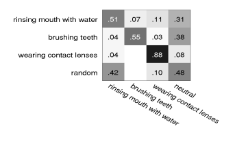
(a) bathroom

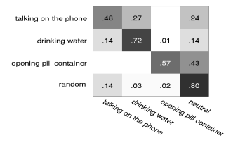
(b) bedroom

(c) kitchen

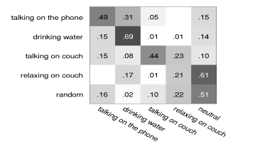
(d) living room

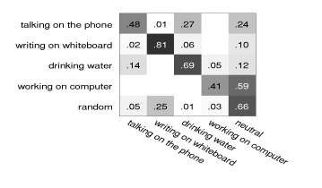
(e) office

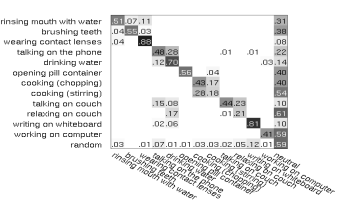
(f) overall

Figure 4: Leave-one-out cross-validation confusion matrix for each location with the full model in the “new person” setting, using skeletal features and skeletal HOG features. The neutral activity denotes that the algorithm estimates that the person is either not doing anything or that the person is engaged in some other activity that we have not defined. The last matrix (bottom-right) shows the results aggregated over all the locations.

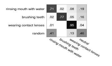
(a) bathroom

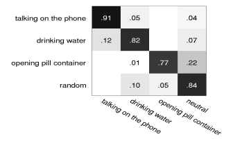
(b) bedroom

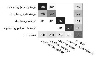
(c) kitchen

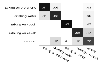
(d) living room

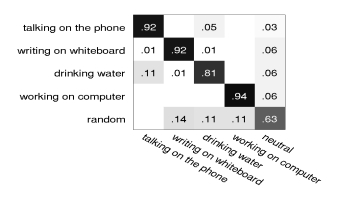
(e) office

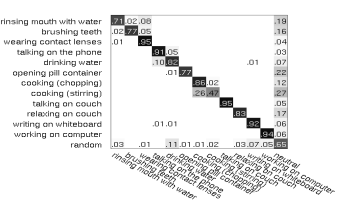
(f) overall

Figure 5: Same format as Figure 4 except it is in the “have seen” setting.

IV-A Results and Discussion

Table I shows the results of the naive classifier, one-level MEMM and our full two-layered model for the “have seen” and “new person” settings. The precision and recall measures are used as metrics for evaluation. Our model was able to detect and classify with a precision/recall measure of 84.7%/83.2% and 67.9%/55.5% in “have seen” and “new person” settings, respectively. It is not surprising that the model performs better in the “have seen” setting, as it has seen that person’s body type and mannerisms before.

We found that both the naive classifier and one-level MEMM were able to classify well when a frame contained distinct characteristics of an activity, but performed poorly when characteristics were subtler. The one-layer MEMM was able to perform better than the naive classifier, as it naturally captures important temporal properties of motion. Our full two-layer MEMM, however, is able to capture the hierarchical nature of human activities in a way that neither the naive classifier nor the one-layer MEMM can do. As a result, it performed the best of all three models.

The comparison of feature sets on our full model shows that the features we use are much more robust compared to features that rely on RGB and/or Depth.

In the “have seen” setting, the HOG on RGB images are capable of capturing powerful information about a person. However, when seeing a new person, changes in clothing and background can cause confusion especially in uncontrolled and cluttered backgrounds, as shown by relatively low precision/recall value of 33.1%/23.5%. The skeletal features along with HOG on depth, while sometimes less informative than the HOG on images, are both more robust to changes in people. Thus, by combining skeletal features, skeletal HOG image features, and skeletal HOG depth features, we simultaneously achieved good accuracy in the “new person” setting and very good accuracy in the “have seen” setting.

Figure 4 and Figure 5 show the confusion matrices between the activities in “new person” and “have seen” setting when using skeletal features and “skeletal HOG” image and depth features. When it did not classify correctly, it usually chose the neutral activity, which is typically not as bad as choosing a wrong “active” activity. When we look at the confusion matrices, we see that many of the mistakes are actually reasonable in that the algorithm confuses them with very similar activities. For example, cooking-chopping and cooking-stirring are often confused, rinsing mouth with water is confused with brushing teeth, and talking on the couch is confused with relaxing on the couch.

Another strength of our model is that it correctly classifies random data as neutral most of the time, as shown in the bottom row of the confusion matrices. This means that it is able to distinguish whether the provided set of activities actually occurs or not—thus our algorithm is not likely to misfire when a person is doing some new activity that the algorithm has not seen before. Also, since we trained on both the regular and mirrored data, the model performs well with both left- and right-handed people.

However, there are some limitations to our method. First, our data only included cases in which the person was not occluded by an object; our method does not model occlusions and may not be robust to such situations. Second, some activities require more contextual information other than simply human pose. For example, knowledge of objects being used could help significantly in making human activity recognition algorithms more powerful in the future.

V Conclusion

In this paper, we considered the problem of detecting and recognizing activities that humans perform in unstructured environments such as homes and offices. We used an inexpensive RGBD sensor (Microsoft Kinect) as the input sensor, the low cost of which enables our approach to be useful for applications such as smart homes and personal assistant robots. We presented a two-layered maximum entropy Markov model (MEMM). This MEMM modeled different properties of the human activities, including their hierarchical nature, the transitions between sub-activities over time, and the relation between sub-activities and different types of features. During inference, our algorithm exploited the hierarchical nature of human activities to determine the best MEMM graph structure. We tested our algorithm extensively on twelve different activities performed by four different people in five different environments, where the test activities were often interleaved with random activities not belonging to these twelve categories. It achieved good detection performance in both settings, where the person was and was not seen before in the training set, respectively.

References

- Boiman and Irani [2005] O. Boiman and M. Irani. Detecting irregularities in images and in video. IJCV, 74(1):17–31, 2005.
- Brand et al. [1997] M. Brand, N. Oliver, and A. Pentland. Coupled hidden makov models for complex action recognition. In CVPR, 1997.
- Bui et al. [2004] H. Bui, D. Phung, and S. Venkatesh. Hierarchical hidden markov models with general state hierarchy. In AAAI, 2004.
- Dalal and Triggs [2005] N. Dalal and B. Triggs. Histograms of oriented gradients for human detection. In CVPR, 2005.
- Demiris and Meltzoff [2008] Y. Demiris and A. Meltzoff. The robot in the crib: a developmental analysis of imitation skills in infants and robots. Infant and Child Development, 17(1):43–53, 2008.
- Dollar et al. [2005] P. Dollar, V. Rabaud, G. Cottrell, and S. Belongie. Behavior recognition via sparse spatio-temporal features. In Int’l Wrksp Visual Surv Perf. Eval. Tracking Surv., 2005.
- Feil-Seifer and Matarié [2005] D. Feil-Seifer and M. J. Matarié. Defining socially assistive robots. In ICORR, 2005.
- Fine et al. [1998] S. Fine, Y. Singer, and N. Tishby. Parsing human motion with stretchable models. Machine Learning, 1998.
- Giese and Poggio [2003] M. Giese and T. Poggio. Neural mechanisms for the recognition of biological movement. Nature Rev Neurosc., 4:179–192, 2003.
- Gupta et al. [2009] A. Gupta, P. Srinivasan, J. Shi, and L. S. Davis. Understanding videos, constructing plots learning a visually grounded storyline model from annotated videos. In CVPR, 2009.
- Jhuang et al. [2007] H. Jhuang, T. Serre, L. Wolf, and T. Poggio. A biologically inspired system for action recognition. In ICCV, 2007.
- Jiang et al. [2012] Y. Jiang, M. Lim, C. Zheng, and A. Saxena. Learning to place new objects in a scene. IJRR, 2012.
- Koppula et al. [2011] H. Koppula, A. Anand, T. Joachims, and A. Saxena. Semantic labeling of 3d point clouds for indoor scenes. In NIPS, 2011.
- Lan et al. [2010] T. Lan, Y. Wang, W. Yang, and G. Mori. Beyond actions: Discriminative models for contextual group activities. In NIPS, 2010.
- Laptev [2005] I. Laptev. On space-time interest points. IJCV, 64(2):107–123, 2005.
- Li et al. [2011] C. Li, T. Wong, N. Xu, and A. Saxena. Feccm for scene understanding: Helping the robot to learn multiple tasks. In Video contribution in ICRA, 2011.
- Li et al. [2007] Z. Li, S. Wachsmuth, J. Fritsch, and G. Sagerer. Vision Systems: Segmentation and Pattern Recognition, chapter 8, pages 131–148. InTech, 2007.
- Liao et al. [2007] L. Liao, D. Fox, and H. Kautz. Extracting places and activities from gps traces using hierarchical conditional random fields. IJRR, 26(1):119–134, 2007.
- Liu et al. [2008] J. Liu, S. Ali, and M. Shah. Recognizing human actions using multiple features. In CVPR, 2008.
- Lopes et al. [2007] M. Lopes, F. S. Melo, and L. Montesano. Affordance-based imitation learning in robots. In IROS, 2007.
- Martinez-Contreras et al. [2009] F. Martinez-Contreras, C. Orrite-Urunuela, E. Herrero-Jaraba, H. Ragheb, and S. A. Velastin. Recognizing human actions using silhouette-based hmm. In AVSS, pages 43–48, 2009.
- Mccallum et al. [2000] A. Mccallum, D. Freitag, and F. Pereira. Maximum entropy markov models for information extraction and segmentation. In ICML, 2000.
- Mutch and Lowe [2006] J. Mutch and D. Lowe. Multiclass object recognition using sparse, localized features. In CVPR, 2006.
- Nguyen et al. [2008] H. Nguyen, C. Anderson, A. Trevor, A. Jain, Z. Xu, and C. C. Kemp. El-e: An assistive robots and fetches objects from flat surfaces. In HRI, 2008.
- Niebles et al. [2010] J. Niebles, C.-W. Chen, and L. Fei-Fei. Modeling temporal structure of decomposable motion segments for activity classification. In ECCV, 2010.
- Ning et al. [2009] H. Ning, T. X. Han, D. B. Walther, M. Liu, and T. S. Huang. Hierarchical space-time model enabling efficient search for human actions. IEEE Trans Circuits Sys. Video Tech., 19(6), 2009.
- PrimeSense [2011] PrimeSense. Nite middleware. http://www.primesense.com/, 2011.
- Ranzato et al. [2007] M. Ranzato, F. J. Huang, Y.-L. Boureau, and Y. LeCun. Unsupervised learning of invariant feature hierarchies with applications to object recognition. In CVPR, 2007.
- Rodriguez et al. [2008] M. D. Rodriguez, J. Ahmed, and M. Shah. Action mach: A spatio-temporal maximum average correlaton height filter for action recognition. In CVPR, 2008.
- Sapp et al. [2011] B. Sapp, D. Weiss, and B. Taskar. Parsing human motion with stretchable models. In CVPR, 2011.
- Saxena et al. [2009] A. Saxena, J. Driemeyer, and A. Ng. Learning 3-d object orientation from images. In ICRA, 2009.
- Serre et al. [2005] T. Serre, L. Wolf, and T. Poggio. Object recognition with features inspired by the visual cortex. In CVPR, 2005.
- Sminchisescu et al. [2005] C. Sminchisescu, A. Kanaujia, Z. Li, and D. Metaxas. Conditional models for contextual human motion recognition. In ICCV, 2005.
- Tapus et al. [2008] A. Tapus, C. Ţăpuş, and M. J. Matarié. User-robot personality matching and assistive robot behavior adaptation for post-stroke rehabilitation therapy. Intel. Ser. Robotics, 1(2):169–183, 2008.
- Theodoridis et al. [2008] T. Theodoridis, A. Agapitos, H. Hu, and S. M. Lucas. Ubiquitous robotics in physical human action recognition: A comparison between dynamic anns and gp. In ICRA, 2008.
- Truyen et al. [2008] T. T. Truyen, D. Q. Phung, H. H. Bui, and S. Venkatesh. Hierarchical semi-markov conditional random fields for recursive sequential data. In NIPS, 2008.
- Wang et al. [2009] X. Wang, X. Ma, and W. Grimson. Unsupervised activity perception in crowded and complicated scenes using hierarchical bayesian models. Pattern Analysis and Machine Intelligence, 2009.
- Weinland et al. [2007] D. Weinland, E. Boyer, and R. Ronfard. Action recognition from arbitrary views using 3d exemplars. In ICCV, 2007.
- Wilson and Bobick [1999] A. D. Wilson and A. F. Bobick. Parametric hidden markov models for gesture recognition. Pattern Analysis and Machine Intelligence, 1999.
- Wong et al. [2007] S.-F. Wong, T.-K. Kim, and R. Cipolla. Learning motion categories using both semantic and structural information. In CVPR, 2007.
- Wu et al. [2007] J. Wu, A. Osuntogun, T. Choudhury, M. Philipose, and J. M. Rehg. A scalable approach to activity recognition based on object use. In ICCV, 2007.