Efficient almost-exact Lévy area sampling

Abstract

We present a new method for sampling the Lévy area for a two-dimensional Wiener process conditioned on its endpoints. An efficient sampler for the Lévy area is required to implement a strong Milstein numerical scheme to approximate the solution of a stochastic differential equation driven by a two-dimensional Wiener process whose diffusion vector fields do not commute. Our method is simple and complementary to those of Gaines–Lyons and Wiktorsson, and amenable to quasi-Monte Carlo implementation. It is based on representing the Lévy area by an infinite weighted sum of independent Logistic random variables. We use Chebychev polynomials to approximate the inverse distribution function of sums of independent Logistic random variables in three characteristic regimes. The error is controlled by the degree of the polynomials, we set the error to be uniformly $10^{-12}$. We thus establish a strong almost-exact Lévy area sampling method. The complexity of our method is square logarithmic. We indicate how it can contribute to efficient sampling in higher dimensions.

1 Introduction

We consider the problem of sampling the Lévy area for a two-dimensional Wiener process $(W^{1}_{t},W^{2}_{t})^{\text{\tiny{T}}}$ conditioned on its endpoints. Indeed, on each computational timestep of size $h$, we must generate two independent sample Wiener increments, $\Delta W^{1}$ and $\Delta W^{2}$, and a sample of the Lévy area

$$A(h)\coloneqq\frac{1}{2}\int_{t}^{t+h}\int_{t}^{\tau_{1}}\,{\mathrm{d}}W^{1}_{\tau_{2}}{\mathrm{d}}W^{2}_{\tau_{1}}-{\mathrm{d}}W^{2}_{\tau_{2}}{\mathrm{d}}W^{1}_{\tau_{1}}.$$

Wiktorsson (2001) proposed approximating the Lévy area, given $\Delta W^{1}$ and $\Delta W^{2}$, by (see Lévy, 1951)

$$\frac{h}{2\pi}\Biggl{[}\sum_{n=1}^{N}\frac{1}{n}\Bigl{(}U_{n}\bigl{(}Y_{n}-\sqrt{\tfrac{2}{h}}\Delta W^{2}\bigr{)}-V_{n}\bigl{(}X_{n}-\sqrt{\tfrac{2}{h}}\Delta W^{1}\bigr{)}\Bigr{)}+\biggl{(}2(1+a^{2})\Bigl{(}\frac{\pi^{2}}{6}-\sum_{n=1}^{N}\frac{1}{n^{2}}\Bigr{)}\biggr{)}^{\frac{1}{2}}\,Z\Biggr{]}.$$

Here $a^{2}\coloneqq\bigl{(}(\Delta W^{1})^{2}+(\Delta W^{2})^{2}\bigr{)}/h$ and $U_{n},V_{n},X_{n},Y_{n}$, for $n=1,\ldots,N$, and $Z$ are independent standard Normal random variables. Without the tail term involving $Z$, it is the Kloeden–Platen–Wright approximation (Kloeden et al., 1992) with mean-square error of order $h^{2}/N$. With Wiktorsson’s tail approximation, the mean-square error improves to $h^{2}/N^{2}$. This method is not restricted to a two-dimensional Wiener process.

In general, to implement a strong Milstein method to approximate the solution of a stochastic differential equation driven by a two-dimensional Wiener process, we must sufficiently accurately strongly sample the Lévy area. We measure the complexity (computational effort) associated with such an approximation by the number of uniform random variables required to generate a Lévy area sample on each timestep of mean-square accuracy $\epsilon$. The smaller the complexity, the more effective is the simulation method. Roughly, for the Kloeden–Platen–Wright method, to achieve accuracy $\epsilon$, we require $N$ of order $h^{2}/\epsilon$. The number of uniform random variables required to generate an approximation truncated at $N$ terms is of order $N$. Hence the complexity is $h^{2}/\epsilon$. For Wiktorsson’s method, the number of uniform samples we require is also of order $N$. However to achieve accuracy $\epsilon$ we require $N$ to be of order $h/\epsilon^{1/2}$, which is a significantly improved complexity. The method proposed by Rydén and Wiktorsson (2001) also has complexity $h/{\varepsilon}^{1/2}$; though see Section 5. The Gaines and Lyons (1994) method is an exact acceptance-rejection method. Hence it cannot be used for quasi-Monte Carlo simulations. It is reported to be “fast but complicated to implement”, see Rydén and Wiktorsson (2001). Stump and Hill (2005) derive a new series representation of the joint distribution function. However in practice, a large number of terms would have to be included to achieve an acceptable accuracy for the distribution function, which would then have to be numerically inverted (see their Section 7).

Our main new result and simulation method is based on the following theorem. The results proved rely on the Lévy characteristic function (Lévy, 1951) for the Lévy area $A(h)$; see Section 4.

Theorem 1.1 (Logistic Expansion).

The Lévy area $A(h)$ conditioned on the Wiener increments $\Delta W^{1}$ and $\Delta W^{2}$ is equivalent in distribution to the series of Logistic random variables $A(h)\sim\lim_{N\to\infty}A_{N}(h)$, where

$$A_{N}(h)\coloneqq\frac{h}{2\pi}\biggl{(}X+\sum_{n=0}^{N}\frac{1}{2^{n}}\sum_{k=1}^{P_{n}}X_{n,k}\biggr{)},$$

where for $n=0,1,\ldots,N$: the $P_{n}\sim\textsf{Poisson}\bigl{(}\tfrac{1}{2}a^{2}2^{n}\bigr{)}$ are independent Poisson random variables, for $k=1,2,\ldots,P_{n}$, $X=\log\bigl{(}U/(1-U)$ and $X_{n,k}=\log\bigl{(}U_{n,k}/(1-U_{n,k})$ with $U,U_{n,k}\sim\textsf{Unif}([0,1])$ independent identically distributed uniform random variables (i.e. $X,X_{n,k}\sim\textsf{Logistic}(1)$ are independent identically distributed Logistic random variables). The mean-square error of the Logistic expansion approximation $A_{N}(h)$ is exactly $a^{2}h^{2}/(3\cdot 2^{N+3})$. The Logistic approximation to $A(h)$ including simulating the tail sum is

$$A_{N}(h)+(ah/\sqrt{3\cdot 2^{N+3}})\,Z,$$

where $Z\sim\textsf{N}(0,1)$. The mean-square error in this approximation is bounded by $h^{2}/(15\cdot 2^{2N+1})$.

In the Logistic approximation in the theorem, at each order $n$, we must on average sample and add $\mathbb{E}\,(P_{n})=\frac{1}{2}a^{2}2^{n}$ Logistic random variables. The strong mean-square error results imply that to achieve accuracy ${\varepsilon}$ we require $N$ such that $2^{N}$ is of order $h^{2}/\epsilon$. Hence the complexity of the Logistic approximation $A_{N}(h)$ is $h^{2}/{\varepsilon}$; with tail simulation it is $h/{\varepsilon}^{1/2}$. However, if we can simulate the sum of say $P\gg 1$ independent Logistic random variables efficiently, then our representation can be used as a basis for an effective Lévy area sampling method; see Section 2 for details. Indeed for $P=10^{3},10^{4},10^{5},10^{6}$ we approximate the inverse distribution function for the sum of $P$ independent Logistic random variables by Chebychev polynomials, in the central, middle and tail regions of the inverse distribution. With this replacement, we still achieve a strong approximation. Our tail region stops at distance $10^{-12}$ from the endpoints. The error of the Chebychev approximations in the three regions is controlled by the degrees of the polynomials we prescribe. We choose to require uniform errors of order $10^{-12}$, which is far smaller than the Monte Carlo error we could achieve, and which we regard as almost-exact. Note to approximate the Lévy area, we truncate the Logistic series representation to include terms with $n\leqslant N$. The mean-square truncation error implies that, as above, we require $N$ such that $2^{N}$ is of order $h^{2}/\epsilon$. However for our truncation we must on average sample order $N^{2}$ uniform random variables—this is the sum over $n\leqslant N$ of the sum of the digits in $\mathbb{E}\,(P_{n})$. Hence the complexity is the square of the logarithm of $h^{2}/\epsilon$ without tail and square logarithm of $h/\epsilon^{1/2}$ with tail; see the electronic supplement for more details. To summarize, the advantages of our direct inversion method based on the Logistic expansion are: (1) its square logarithmic complexity and (2) the main ingredient is direct inversion, which importantly, can be used in combination with quasi-Monte Carlo simulation.

2 Direct inversion algorithm

We apply the ideas underlying the Beasley–Springer–Moro method for standard Normal random variables. More details, including comprehensive details of anaylsis and tables of polynomial coefficients, can be found in the electronic supplement. We consider the fixed values $P=10^{3},10^{4},10^{5},10^{6}$. Let $\Phi$ denote the distribution function for the sum of $P$ independent Logistic random variables. The inverse distribution function $\Phi^{-1}=\Phi^{-1}(u)$ is antisymmetric about $1/2$. We thus focus on the subinterval $[1/2,1)$ of its support. Indeed we split this interval into the three regions: the central $[1/2,u_{1}]$; middle $(u_{1},u_{2}]$ and tail $(u_{2},1-10^{-12}]$ regions. We neglect the regions at distance $10^{-12}$ from the endpoints. The values $u_{1}=u_{1}(P)$ and $u_{2}=u_{2}(P)$ roughly separate the characteristic behaviour of $\Phi^{-1}$. In the central region we approximate $\Phi^{-1}\approx U\cdot C_{n}(z)$ where $C_{n}$ is a degree $n$ Chebychev polynomial approximation, where $U\coloneqq(2P\pi^{3}/3)^{1/2}(u-1/2)$ and $z=k_{1}U^{2}+k_{2}$. In the middle and tail regions we approximate $\Phi^{-1}\approx C_{n}(z)$ where $z=k_{1}U+k_{2}$ and $U\coloneqq\pi\bigl{(}-\frac{2}{3}P\log(2\sqrt{\pi}(1-u))\bigr{)}^{1/2}$. Briefly the rationale underlying this ansatz for $U$ is as follows. By the Central Limit Theorem, asymptotically in distribution, we have $\Phi(x)\sim\Phi_{\mathrm{N}}\bigl{(}x/\pi\,(P/3)^{1/2}\bigr{)}$, where $\Phi_{\mathrm{N}}$ is the standard Normal distribution function. Following Moro (1995), using the asymptotic tail approximation for the standard Normal, we find $\Phi(x)\sim 1-(1/2\pi^{1/2})\exp(-x^{2}/(2\pi^{2}P/3))$. Inverting this relation gives the ansatz for $U$. Note, in all three regions, $k_{1}$ and $k_{2}$ are chosen to ensure $z=-1$ at the left endpoint and $z=+1$ at the right endpoint.

The coefficients for the Chebychev polynomial approximations are computed in the standard fashion, see Section 5.8 in Press et al. (1992). However two additional aspects are crucial to their accurate and efficient evaluation. First, based on the inverse Fourier transform of the characteristic function for the sum of $P$ Logistic random variables, we derived a large $P$ asymptotic approximation for the distribution function $\Phi=\Phi(x)$. Following Bender and Orszag (1999, pp. 272–4) we developed the expansion in reciprocal powers of $P$ to all orders. Indeed we computed up to $140$ terms to obtain the requisite accuracy for $\Phi$ in the tail regions. Second, we computed the expansion and performed the required rootfinding for $\Phi^{-1}$ values using Maple with $25$ (and on occasion $45$) digit accuracy. We imported these accurate and reliable Chebychev coefficients to Matlab. All subsequent computations are done using double precision in Matlab—the Chebychev approximations were evaluated using Clenshaw’s recurrence formula (Press et al., 1992, p. 193). Figure 1 shows the errors in the Chebychev polynomial approximations for $\Phi^{-1}$ across all three regions when $P$ is $10^{3}$ and $10^{6}$. The Chebychev polynomials have degrees from $13$ to $15$ in the centre (roughly $[0.5,0.8]$) and middle regions (roughly $[0.8,0.95]$), and degrees $24$ to $26$ in the tail region.

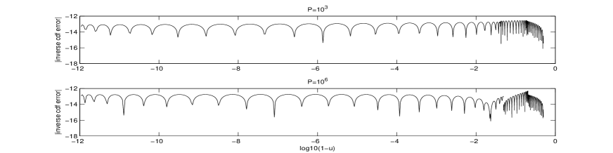
Figure 1: The panels show the error in the Chebychev polynomial approximations to $\Phi^{-1}=\Phi^{-1}(u)$ for $P=10^{3}$ (top) and $P=10^{6}$ (bottom) across all three regions with $u\in[1/2,1-10^{-12}]$. Note we use $1-u$ on the abscissa and a $\log$-$\log_{10}$ plot to highlight the tail region (on the left).

The direct inversion algorithm works as follows. We use the Logistic series representation in Theorem 1.1 which we truncate at some large integer $N$. First, consider the Poisson samples $P_{n}$ required for each $n=0,\ldots,N$. These are obtained by direct inversion when the mean $\frac{1}{2}a^{2}2^{n}$ is $100$ or less—rather than faster acceptance-rejection methods. For means $100$ or greater, we use the PTRS transformed rejection (or almost-exact inversion) method from Hörmann (1993). To achieve an almost-exact quasi-Monte Carlo implementation, tables of the Poisson distribution function could be constructed for different representative means such as $10^{i}$ for $3\leqslant i\leqslant 12$. Since the standard deviation of a Poisson random variable is the square-root of the mean, such tables which ignore tails of order $10^{-12}$ will not be restrictively large. Samples can be drawn for these representative means by a fast look-up algorithm. A Poisson sample for a given mean could be generated by adding the requisite numbers of Poisson samples from the representative means. Second, the sums of $P_{n}$ Logistic random variables are handled thus. Whenever $P_{n}<10^{3}$ we sum $P_{n}$ Logistic random variables. However if $P_{n}\geqslant 10^{3}$ we decompose $P_{n}=p+p_{3}\cdot 10^{3}+p_{4}\cdot 10^{4}+p_{5}\cdot 10^{5}+p_{6}\cdot 10^{6}$. Here $p=P_{n}\,\text{mod}\,10^{3}$ and the $p_{k}$ are the multiples of $10^{k}$ present in the sample $P_{n}$; note $p_{6}$ need not be a single digit. For each $k=3,4,5,6$ we sample $p_{k}$ random variables from the distribution function for the sum of $10^{k}$ Logistic random variables using the corresponding Chebychev polynomial approximations described above.

3 Simulations

We simulated the Lévy area $A(h)$ using three methods with and without tail simulation for $h=1$. These are: Kloeden–Platen–Wright from the introduction (no tail); Logistic method using Theorem 1.1 where the requisite Poisson number of Logistic random variables are added at each order $n=0,\ldots,N$ and direct inversion based on the Logistic expansion as described in Section 2. We also implemented these three methods with tail simulation as shown in the introduction and Theorem 1.1, respectively. In Figure 2 the panels show the absolute error in the second moment (left) and fourth moment (right) versus the CPU time required to compute the simulation. Since $\mathbb{E}\,a^{2}=\mathbb{E}\,\bigl{(}(\Delta W^{1})^{2}+(\Delta W^{2})^{2}\bigr{)}/h=2$ and $h=1$, the true variance $(1+\mathbb{E}\,a^{2})\,h^{2}/12$ is $1/4$. The exact fourth moment is $5/16$.

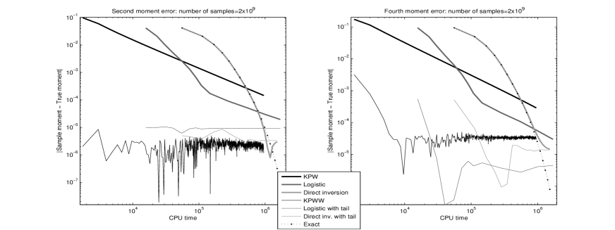
Figure 2: We show the absolute error in the second (left) and fourth (right) moments versus the CPU time required to compute the simulation for three different methods (with and without tail simulation). The methods are: Kloeden–Platen–Wright (KPW); Logistic method based on adding the requisite Logistic random variables; direct inversion based on the Logistic expansion; Kloeden–Platen–Wright–Wiktorsson (KPWW); Logistic expansion with tail simulation and direct inversion with tail simulation. We fixed $h=1$, hence the exact second and fourth moments are $1/4$ and $5/16$, respectively. The corresponding exact error in these moments for the direct inversion method is also indicated.

We performed $L=2\times 10^{9}$ simulations in all cases. The Monte Carlo error is of order $L^{-1/2}$. This can be observed in Figure 2, where the error curves become “horizontal and noisy”. For all methods we truncated after $N$ terms, increasing $N$ in integers for the Kloeden–Platen–Wright method, and in powers of $2$ for the Logistic and direct inversion methods. We included $N=2^{10},2^{13}$ and $2^{18}$ terms for the Kloeden–Platen–Wright, Logistic and direct inversion methods, respectively. The errors of the sample moments in the basic approximations in Figure 2 are in good correspondence with their theoretical values. We observe this for example, for the direct inversion method for which we also plot the exact second and fourth moment errors versus the corresponding simulation CPU times (the fourth moment error calculation can be found in the electronic supplement). In particular we observe the behaviour of the exact error in the large $N$ regime, where the simulations are dominated by the Monte Carlo error. We also observe the complexity of $\varepsilon^{-1}$ for the Kloeden–Platen–Wright and Logistic expansion methods (without tail simulation). In the Logistic method case this complexity is observed in the high accuracy/large effort asymptotic limit. Although the direct inversion method requires more effort at low accuracies, the square logarithmic complexity is observed in the high accuracy/large effort asymptotic limit. In each method the tail approximations are designed so that the tail is approximated by a matched Normal random variable (the first two moments are matched). Hence they simulate the second moment exactly and we only observe Monte Carlo noise on the left in Figure 2. The simulations thus confirm the analysis and expected properties.

4 Proof of the Logistic Expansion Theorem

The characteristic function $\hat{\phi}=\hat{\phi}(\xi)$ corresponding to the probability density function $\phi$ for the Lévy area $A(h)$, given $\Delta W^{1}$ and $\Delta W^{2}$, is $\hat{\phi}(\xi)=\bigl{(}\tfrac{1}{2}h\xi/\sinh(\tfrac{1}{2}h\xi)\bigr{)}\exp\bigl{(}-\tfrac{1}{2}a^{2}\bigl{(}\tfrac{1}{2}h\xi\coth(\tfrac{1}{2}h\xi)-1\bigr{)}\bigr{)}$. We observe the identity $\mathrm{coth}\,z\equiv\mathrm{coth}\,z/2-1/\mathrm{sinh}\,z$, iterated $N$ times, generates the identity $\mathrm{coth}\,z\equiv\mathrm{coth}(z/2^{N+1})-\sum_{n=0}^{N}1/\mathrm{sinh}(z/2^{n})$. Substituting this identity into the characteristic function we see that

$$\exp\bigl{(}-\tfrac{1}{2}a^{2}(z\,\mathrm{coth}\,z-1)\bigr{)}=\prod_{n=0}^{N}\exp\biggl{(}\tfrac{1}{2}a^{2}2^{n}\cdot\frac{z/2^{n}}{\mathrm{sinh}\,z/2^{n}}\biggl{)}\exp\bigl{(}-\tfrac{1}{2}a^{2}2^{n}\bigr{)}\cdot\exp\bigl{(}\mathcal{E}_{N}(z,a)\bigr{)},$$

where $\mathcal{E}_{N}(z,a)\coloneqq-\tfrac{1}{2}a^{2}\bigl{(}z\,\mathrm{coth}\,(z/2^{N+1})-2^{N+1}\bigr{)}\to 0$ as $N\to\infty$, $\forall\,z\in\mathbb{R}$. Thus $\forall\,z=\xi h/2\in\mathbb{R}$, we have

$$\hat{\phi}(\xi)=\frac{\xi h/2}{\mathrm{sinh}\,\xi h/2}\cdot\prod_{n=0}^{\infty}\mathbb{E}\,\biggl{(}\frac{\xi h/2^{n+1}}{\mathrm{sinh}\,\xi h/2^{n+1}}\biggr{)}^{P_{n}},$$

where $P_{n}\sim\textsf{Poisson}\bigl{(}\tfrac{1}{2}a^{2}2^{n}\bigr{)}$. Note that the expression $(\xi h/2^{n+1})/\mathrm{sinh}(\xi h/2^{n+1})$ is the characteristic function of a $\textsf{Logistic}(h/2^{n+1}\pi)\sim(h/2^{n+1}\pi)\cdot\textsf{Logistic}(1)$ random variable. The Logistic expansion follows.

We now focus on the error statements. First consider the tail sum itself. Directly computing

$$\mathbb{E}\,\bigl{|}A(h)-A_{N}(h)\bigr{|}^{2}=\mathbb{E}\,\biggl{(}\frac{h}{2\pi}\sum_{n=N+1}^{\infty}\frac{1}{2^{n}}\sum_{k=1}^{P_{n}}X_{n,k}\biggr{)}^{2}=\Bigl{(}\frac{h}{2\pi}\Bigr{)}^{2}\sum_{n=N+1}^{\infty}\frac{1}{2^{2n}}\sum_{l=0}^{\infty}\mathbb{P}\,\{P_{n}=l\}\cdot\mathbb{E}\,\biggl{(}\sum_{k=1}^{l}X_{n,k}\biggr{)}^{2}.$$

Now we use that the expectation on the far right equals $\ell\pi^{2}/3$ and that $\sum_{l\geqslant 0}\mathbb{P}\,\{P_{n}=l\}\cdot l=\mathbb{E}\,\{P_{n}\}=a^{2}2^{n-1}$. Then noting that $\sum_{n\geqslant N+1}2^{-2n}=2^{-(N+1)}$ gives the exact mean-square error result.

Second, we derive the error bound for the approximation including the Normal tail sum approximation. The tail sum is an infinitely divisible class G random variable, i.e. its characteristic function has the form $\hat{\phi}(\xi)=\exp(-\Psi(\xi^{2}))$, where $\Psi(0)=0$, and $(-1)^{n-1}\Psi^{(n)}(\xi)\geq 0$ for all $n$, see Rydén and Wiktorsson (2001) (pg. 163). Using that $A(h)-A_{N}(h)=\frac{h}{2\pi}\sum_{n\geqslant N+1}2^{-n}\sum_{k=1}^{P_{n}}X_{n,k}=\frac{\tilde{h}}{2\pi}\sum_{n\geqslant 0}2^{-n}\sum_{k=1}^{Q_{n}}X_{n,k}$, where $\tilde{h}=h/2^{N+1}$, and where $Q_{n}$ has a Poisson distribution with parameter $\frac{1}{2}\tilde{a}^{2}2^{n}$ and where $\tilde{a}^{2}=a^{2}2^{N+1}$, it follows that the tail sum $A(h)-A_{N}(h)$ has the characteristic function (Lévy, 1951) $\hat{\phi}_{N}(\xi)=\exp\bigl{(}-\tfrac{1}{2}\tilde{a}^{2}\bigl{(}\tfrac{1}{2}\tilde{h}\xi\coth(\tfrac{1}{2}\tilde{h}\xi)-1\bigr{)}\bigr{)}=\exp\bigl{(}-\tfrac{1}{2}\tilde{a}^{2}\sum_{n=1}^{\infty}\xi^{2}/\bigl{(}(n\tilde{h}/2\pi)^{2}+\xi^{2}\bigr{)}\bigr{)}$. Hence $A(h)-A_{N}(h)$ has class G distribution—see also Prop. 5 in Rydén and Wiktorsson (2001). We can now proceed as in the proof of Theorem 7 in Rydén and Wiktorsson. The tail sum can be represented as a product of a standard Normal random variable $Z$ and the square root of an independent positive, infinitely divisible variable $Y_{N}$, i.e. $A(h)-A_{N}(h)=Z\sqrt{Y_{N}}$. If $\sigma_{N}^{2}$ denotes the variance of $A(h)-A_{N}(h)$, then the mean-square error when including the Normal tail approximation is given by

$$\mathbb{E}\,\bigl{|}A(h)-A_{N}(h)-\sigma_{N}Z\bigr{|}^{2}=\mathbb{E}\,\{Z^{2}\}\cdot\mathbb{E}\,\bigl{|}\sqrt{Y_{N}}-\sigma_{N}\bigr{|}^{2}=\mathbb{E}\,(Y_{N}-\sigma_{N}^{2})^{2}/(\sqrt{Y_{N}}+\sigma_{N})^{2}.$$

This is bounded above by $\mathbb{E}\,\bigl{(}Y_{N}-\sigma_{N}^{2}\bigr{)}^{2}/\sigma_{N}^{2}$. Let $g$ denote the Laplace transform of $Y_{N}$. Then $g(z)=\hat{\phi}_{N}(\sqrt{2z})$, and the variance of $Y_{N}$ is given by $(\log g)^{\prime\prime}(0)$. If $\ell(z)\coloneqq 1-\sqrt{2z}\coth(\sqrt{2z})$ then we see that $\log g(z)=\tilde{a}^{2}\ell(z\tilde{h}^{2}/4)$ and $(\log g)^{\prime\prime}(0)=\tilde{a}^{2}(\tilde{h}/2)^{4}\ell{{}^{\prime\prime}}(0)$. Hence the mean-square error when including tail approximation is bounded by $\sigma_{N}^{-2}\tilde{a}^{2}(\tilde{h}/2)^{4}\ell^{\prime\prime}(0)=h^{2}/(15\cdot 2^{2N+1})$, completing the proof.

5 Conclusion

We conclude with some brief observations. For low to medium accuracies the Kloeden–Platen–Wright–Wiktorsson and Logistic expansion methods perform extremely well. When high accuracies are required and/or a quasi-Monte Carlo implementation is intended, then the almost-exact direct inversion method is the method of choice as can be observed in Figure 2. In the electronic supplement we provide more detailed complexity calculations in order to establish a cross-over accuracy criterion. In other words we specify the accuracy for which one would preferentially use the direct inversion over the Kloeden–Platen–Wright–Wiktorsson method. This depends of course on an efficient implmentation of the algorithm and the system on which it is implemented. Though we endeavoured to establish the three regions and Chebychev polynomial approximations for each $P$ so that the direct inversion algorithm is efficient, they could be further optimized. Note for example, for our simulation implementation in Figure 2 for medium accuracies we would preferentially use the basic Logistic method. The direct inversion techniques above could also be applied to the Rydén–Wiktorsson series which involves large sums of independent Laplace random variables. Lastly, we remark on the case of a $d$-dimensional Wiener process with $d\geqslant 3$. When $d=3$, the characteristic variable is $Z\in\mathfrak{so}(3)$ and $Z^{3}=-\|{\boldsymbol{z}}\|^{2}\,Z$, where $\|{\boldsymbol{z}}\|$ is the Euclidean norm of the vector ${\boldsymbol{z}}$ of the three upper triangular components of $Z$. This property simplifies power series functions of $Z$ with scalar coefficients and underlies Rodrigues formulae for $Z\in\mathfrak{so}(3)$. Such formulae generalize to higher dimensions; see Gallier and Xu (2002). In particular, the joint characteristic function given by Wiktorsson (2001) for the Lévy areas $A_{12}$, $A_{13}$ and $A_{23}$ conditioned on $\Delta\boldsymbol{W}\coloneqq(\Delta W^{1},\Delta W^{2},\Delta W^{3})^{\text{\tiny{T}}}$ reduces to (scaling ${\boldsymbol{z}}$ by $h/2$)

$$\frac{\|{\boldsymbol{z}}\|}{\sinh\|{\boldsymbol{z}}\|}\cdot\exp\bigl{(}-\tfrac{1}{2}\|\Delta\boldsymbol{W}\|^{2}\,(\|{\boldsymbol{z}}\|\,\mathrm{coth}\|{\boldsymbol{z}}\|-1)\bigr{)}\cdot\exp\bigl{(}\tfrac{1}{2}\|\Delta\boldsymbol{W}\|^{2}\,\langle\Delta\hat{\boldsymbol{W}},\hat{\boldsymbol{z}}\rangle^{2}\,(\|{\boldsymbol{z}}\|\,\mathrm{coth}\|{\boldsymbol{z}}\|-1)\bigr{)}.$$

Here $\langle\Delta\hat{\boldsymbol{W}},\hat{\boldsymbol{z}}\rangle$ is the Euclidean inner product of the corresponding unit vectors. This result can be found in Mansuy and Yor (2008, p. 23). The first factor is the characteristic function of a generalized Logistic random variable and the second (radial-type) factor can be analysed in the same fashion as we have presented here. Appropriately efficiently simulating the third (angular-type) factor is our next goal.

Supplementary material

We present comprehensive details underlying some of the results in our manuscript. We include: (1) a derivation of the exact error in the fourth moment; (2) an accuracy criterion which indicates when, in terms of complexity, it is more preferential to use the direct inversion over Kloeden–Platen–Wright–Wiktorsson method; and for a sum of Logistic random variables, we include (3) the derivation of the distribution function representation in the large sum asymptotic limit; (4) complete tables of the coefficients used for the Chebychev polynomial approximations for the inverse distribution function and (5) the derivation of a finite representation for the density function.

(1) Fourth moment error

In the main text we plotted the exact error in the fourth moment of the Logistic expansion versus CPU time from simulations for the direct inversion method—see Figure 2 (right panel). The analytical expression for the exact error is as follows.

Lemma 5.1.

The error in the fourth moment of the approximation $A_{N}(h)$ to the Lévy area $A(h)$, given $a^{2}\coloneqq\bigl{(}(\Delta W^{1})^{2}+(\Delta W^{2})^{2}\bigr{)}/h$, is

$$\mathbb{E}\,\bigl{(}A_{N}(h)^{4}\bigr{)}-\mathbb{E}\,\bigl{(}A(h)^{4}\bigr{)}=\frac{a^{2}h^{2}}{2^{N+4}}\cdot\biggl{(}-\frac{1}{3}(1+a^{2})+\frac{a^{2}}{12\cdot 2^{N}}-\frac{1}{30\cdot 4^{N}}\biggr{)}.$$

Proof.

First we note that the fourth moment of the Lévy area is given by the fourth derivative of the characteristic function evaluated at the origin. This can be straightforwardly be computed and is given by

$$\mathbb{E}\,\bigl{(}A(h)^{4}\bigr{)}=\frac{1}{2^{4}}\Bigl{(}\frac{7}{15}+\frac{14}{15}a^{2}+\frac{1}{3}a^{4}\Bigr{)}.$$

Second we compute $\mathbb{E}\,\bigl{(}A_{N}(h)^{4}\bigr{)}$. For convenience we set

$$Y_{0}\coloneqq X\qquad\text{and}\qquad Y_{n+1}\coloneqq\frac{1}{2^{n}}\sum_{k=1}^{P_{n}}X_{n,k}$$

for $n=0,1,\ldots,N$, so that $A_{N}(h)$ can be expressed in the form

$$A_{N}(h)=\frac{h}{2\pi}\sum_{n=0}^{N+1}Y_{n}.$$

Here, as stated in the Logistic Expansion Theorem in the main text, the $X$ and $X_{n,k}$ are independent identically distributed Logistic random variables and the $P_{n}$ are independent Poisson random variables with expectation $\frac{1}{2}a^{2}2^{n}$. Hence explicitly we have

$$\mathbb{E}\,\bigl{(}A_{N}(h)^{4}\bigr{)}= \;\Bigl{(}\frac{h}{2\pi}\Bigr{)}^{4}\cdot\mathbb{E}\,\biggl{(}\sum_{n=0}^{N+1}Y_{n}\biggr{)}^{4}$$

$$= \;\Bigl{(}\frac{h}{2\pi}\Bigr{)}^{4}\cdot\biggl{(}\sum_{n=0}^{N+1}\mathbb{E}\,Y_{n}^{4}+6\sum_{n=0}^{N}\sum_{m=n+1}^{N+1}\mathbb{E}\,Y_{n}^{2}\cdot\mathbb{E}\,Y_{m}^{2}\biggr{)}.$$

Note that $\mathbb{E}\,Y_{0}^{2}=\pi^{2}/3$ and $\mathbb{E}\,Y_{0}^{4}=7\pi^{4}/15$. For $n=1,\ldots,N+1$, similar to the error statement calculations in the proof of the Logistic Expansion Theorem in Section 4 of the main text, we have

$$\mathbb{E}\,Y_{n}^{2} \;=\frac{1}{2^{2(n-1)}}\cdot\mathbb{E}\,\biggl{(}\sum_{k=1}^{P_{n-1}}X_{n-1,k}\biggr{)}^{2}$$

$$\;=\frac{1}{2^{2(n-1)}}\cdot\mathbb{E}\,\{P_{n-1}\}\cdot\frac{\pi^{2}}{3}$$

$$\;=\frac{1}{2^{2(n-1)}}\cdot\frac{1}{2}a^{2}2^{n-1}\cdot\frac{\pi^{2}}{3}.$$

Further we can similarly compute for $n=1,\ldots,N+1$:

$$\mathbb{E}\,Y_{n}^{4} \;=\frac{1}{2^{4(n-1)}}\cdot\mathbb{E}\,\biggl{(}\sum_{k=1}^{P_{n-1}}X_{n-1,k}\biggr{)}^{4}$$

$$\;=\frac{1}{2^{4(n-1)}}\cdot\sum_{\ell=0}^{\infty}\mathbb{P}\,\{P_{n-1}=\ell\}\cdot\mathbb{E}\,\biggl{(}\sum_{k=1}^{\ell}X_{n-1,k}\biggr{)}^{4}$$

$$\;=\frac{1}{2^{4(n-1)}}\cdot\sum_{\ell=0}^{\infty}\mathbb{P}\,\{P_{n-1}=\ell\}\cdot\Bigl{(}\frac{7\pi^{4}}{15}\ell+6\cdot\frac{\pi^{4}}{9}\cdot\frac{1}{2}\ell(\ell-1)\Bigr{)}$$

$$\;=\frac{1}{2^{4(n-1)}}\frac{\pi^{4}}{3}\cdot\sum_{\ell=0}^{\infty}\mathbb{P}\,\{P_{n-1}=\ell\}\cdot\Bigl{(}\ell^{2}+\frac{2}{5}\ell\Bigr{)}$$

$$\;=\frac{1}{2^{4(n-1)}}\frac{\pi^{4}}{3}\cdot\mathbb{E}\,\Bigl{\{}P_{n-1}^{2}+\frac{2}{5}P_{n-1}\Bigr{\}}$$

$$\;=\frac{1}{2^{4(n-1)}}\frac{\pi^{4}}{3}\cdot\Bigl{(}\Bigl{(}\frac{1}{2}a^{2}2^{n-1}+\frac{1}{4}a^{4}2^{2(n-1)}\Bigr{)}+\frac{2}{5}\cdot\frac{1}{2}a^{2}2^{n-1}\Bigr{)}$$

$$\;=\frac{1}{2^{4(n-1)}}\frac{\pi^{4}}{3}\cdot\Bigl{(}\frac{1}{4}a^{4}2^{2(n-1)})+\frac{7}{10}a^{2}2^{n-1}\Bigr{)}.$$

Using these last two results in our expression for $\mathbb{E}\,\bigl{(}A_{N}(h)^{4}\bigr{)}$ above we find

$$\mathbb{E}\,\bigl{(}A_{N}(h)^{4}\bigr{)}= \;\Bigl{(}\frac{h}{2}\Bigr{)}^{4}\cdot\biggl{(}\frac{7}{15}+\sum_{n=1}^{N+1}\frac{1}{3}\Bigl{(}\frac{1}{4}a^{4}2^{-2(n-1)})+\frac{7}{10}a^{2}2^{-3(n-1)}\Bigr{)}$$

$$\;\qquad\qquad\quad\;+6\sum_{m=1}^{N+1}\frac{1}{3}\cdot\frac{1}{3}\cdot\frac{1}{2}a^{2}2^{-(m-1)}+6\sum_{n=1}^{N}\sum_{m=2}^{N+1}\frac{1}{9}\cdot\frac{1}{4}a^{4}2^{-(n+m-2)}\biggr{)}$$

$$= \;\Bigl{(}\frac{h}{2}\Bigr{)}^{4}\cdot\biggl{(}\frac{7}{15}+a^{2}\Bigl{(}\frac{14}{15}-\frac{2}{3}2^{-N-1}+\frac{4}{15}8^{-N-1}\Bigr{)}+a^{4}\Bigl{(}\frac{1}{3}-\frac{1}{3}2^{-N}+\frac{1}{3}4^{-N-1}\Bigr{)}\biggr{)},$$

where we used the formula for partial geometric sums. Taking the difference of this result with the expression above for $\mathbb{E}\,\bigl{(}A(h)^{4}\bigr{)}$ we establish the result. ∎

Remark 5.2.

Note that in Figure 2 we take $h=1$ and use that $\mathbb{E}\,a^{2}=2$ and $\mathbb{E}\,a^{4}=8$.

Remark 5.3.

Using analogous arguments to those in the proof of the Logistic Expansion Theorem in Section 4 of the main text and some of the results above, it is straightforward to derive an exact analytical expression for $\mathbb{E}\,|A(h)-A_{N}(h)|^{4}$. We can also derive an upper bound for $\mathbb{E}\,|A(h)-A_{N}(h)-\sigma_{N}Z|^{4}$, where $\sigma_{N}Z$ represents the approximation to the tail sum (as in the main text).

(2) Accuracy criterion

At what accuracy is the complexity of the direct inversion method based on the Logistic expansion better than the Kloeden–Platen–Wright–Wiktorsson method? As mentioned before this depends on how the algorithms are implemented and what system they are implemented on. We use the number of uniform random variables required to generate a Lévy area sample on each timestep to achieve a mean-square accuracy of ${\varepsilon}$, as the measure of complexity. Consider the Kloeden–Platen–Wright method. At leading order the mean-square error, when we truncate the series to include the terms $n\leqslant N$, is equal to $C_{\mathrm{KPW}}\cdot h^{2}/N$, where $C_{\mathrm{KPW}}$ is a known constant. Equating the mean-square error with ${\varepsilon}$, we see that to achieve a mean-square accuracy of ${\varepsilon}$ we must choose $N=C_{\mathrm{KPW}}\cdot h^{2}/{\varepsilon}$. The computational effort required to generate the truncated series is at leading order given by $A_{\mathrm{KPW}}\cdot N$, where $A_{\mathrm{KPW}}$ is a positive constant. Indeed at each order, for each term we need to generate $4$ uniform random variables (for each of the $4$ standard normal random variables required) and we need to also account for the flops and function evaluations required to compute the term. We absorb these factors multiplicatively into the constant $A_{\mathrm{KPW}}$. Hence the Kloeden–Platen–Wright method complexity is

$$B_{\mathrm{KPW}}\cdot h^{2}/{\varepsilon},$$

where we set $B_{\mathrm{KPW}}\coloneqq A_{\mathrm{KPW}}\cdot C_{\mathrm{KPW}}$.

For the direct inversion method based on the Logistic expansion the mean-square error at leading order when we truncate to include the terms $n\leqslant N$, is equal to $C_{\mathrm{DI}}\cdot h^{2}/2^{N}$, where $C_{\mathrm{DI}}=a^{2}/24$. Again, equating the mean-square error with ${\varepsilon}$, to achieve a mean-square accuracy of ${\varepsilon}$ we must choose $N=\log(a^{2}h^{2}/24\,{\varepsilon})/\log 2$. We postulate that the computational effort required to generate this approximation for the direct inversion method has the general quadratic form

$$A+BN+CN^{2},$$

for some constants $A$, $B$ and $C$ dependent on the implementation. Hence the complexity of the direct inversion method has this form with $N=\log(a^{2}h^{2}/24\,{\varepsilon})$, absorbing $1/\log 2$ factors into the constants. The rationale for this quadratic form is as follows. For each $n\leqslant N$ we generate a Poisson random variable $P_{n}$ whose expectation is proportional to $a^{2}2^{n}$. Using direction inversion for the distribution functions of large sums of independent identically distributed Poisson random variables, the number of uniform random variables we need to generate is proportional to the sum of digits in $P_{n}$ which is proportional to $n$. Hence for all the terms $n\leqslant N$, the total number of uniform random variables we need to generate is proportional to $N(N-1)$. Further, in Figure 2 in the main text we observe for small values of $N$, there is a non-negligible additive shift in the direct inversion complexity compared to the basic Logistic method. This is largely due to the algorithm for splitting the Poisson random variable into its digits (which requires further optimization). Hence we include $N^{1}$ and $N^{0}$ dependent terms in our complexity form.

The direct inversion complexity is less than the Kloeden–Platen–Wright complexity when

$$A+B\cdot\bigl{(}\log(a^{2}h^{2}/24\,{\varepsilon})\bigr{)}+C\cdot\bigl{(}\log(a^{2}h^{2}/24\,{\varepsilon})\bigr{)}^{2}<B_{\mathrm{KPW}}\cdot h^{2}/{\varepsilon}.$$

All the quantities involved are known with the exception of the constants $B_{\mathrm{KPW}}$, $A$, $B$ and $C$. These encode the flops and function evaluations required to compute the direct inversion and Kloeden–Platen–Wright samples. They depend on the efficiency of the algorithms implemented, programming language used and the hardware utilized. The Kloeden–Platen–Wright method is very simple and these factors are unlikely to influence $B_{\mathrm{KPW}}$ (indeed they do not; see below). However as we mentioned in the Conclusion of the main text and above, the implementation of the direct inversion method we advocate can be further optimized (though we endeavoured to implement it as efficiently as we could using compiled Matlab code). The constants importantly affect the crossover accuracy below which the inequality above holds.

Let us estimate the crossover accuracy in the context of our implementation generating Figure 2 in the main text—note the Lévy area and the approximations considered here have zero mean and are sums of independent random variables, so the mean-square error and difference of their second moments are the same. Recall that we set $h=1$ and that $\mathbb{E}\,a^{2}=2$. The log-log plot in Figure 2 reveals the $B_{\mathrm{KPW}}/{\varepsilon}$ behaviour we expect for the Kloeden–Platen–Wright method. The mean-square error, from the analytical formula in the Introduction in the main text, for the case $N=2^{9}$ is $2.9655\times 10^{-4}$. The corresponding CPU time from our simulations is $4.7533\times 10^{5}$. Hence we have $B_{\mathrm{KPW}}=1.4096\times 10^{2}$. In Figure 3 in this supplement, we plot accuracy ${\varepsilon}$ versus $B_{\mathrm{KPW}}/{\varepsilon}$ for this value of $B_{\mathrm{KPW}}$ and note a markedly close fit to the simulation error versus CPU time plot. The exact mean-square error plotted versus the simulation CPU times very closes fits the simulation error versus CPU time plot. There is thus very good agreement between the simulations and our leading order complexity expression for the Kloeden–Platen–Wright method. For the direct inversion method we match the quadratic logarithmic form $A+BN+CN^{2}$ with $N=\log(1/12\,{\varepsilon})$ to the three simulation data points corresponding to $N$ equal to $1$, $9$ and $18$, where respectively the exact accuracy ${\varepsilon}$ is $2^{-1}/12$, $2^{-9}/12$ and $2^{-18}/12$ and the corresponding CPU times are $5.5585\times 10^{4}$, $5.8620\times 10^{5}$ and $1.5223\times 10^{6}$. With these values we deduce $A=9.2103\times 10^{3}$, $B=1.4669\times 10^{5}$ and $C=2.4465\times 10^{4}$. We see in Figure 3 in this supplement, this fitted quadratic logarithmic form plotted with complexity on the abscissa and accuracy on the ordinate, fits the error versus CPU time plot very closely. In particular, we have established direct practical confirmation of our main complexity claims for the direct inversion method. Further we can compute the smallest root of $B_{\mathrm{KPW}}/{\varepsilon}-(A+BN+CN^{2})$ with $N=\log(1/12\,{\varepsilon})$, which is $10^{-3.5728}$ (which can be observed in Figure 3). For accuracies below this value, for our implementation, the direct inversion method is more efficient than the Kloeden–Platen–Wright method. With further optimization of the direct inversion implementation, we expect this value to increase.

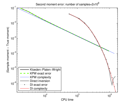
Figure 3: We show the absolute error in the second moment versus the CPU time required to compute the simulation for the Kloeden–Platen–Wright method (KPW) and direct inversion method based on the Logistic expansion (DI), as well as the exact error for the DI method—these are the same as in Figure 2 in the main text. However in addition we include here the exact error for the KPW method and the expressions for the complexity at leading order (abscissa) plotted versus accuracy (ordinate) for the KPW method, $B_{\mathrm{KPW}}/{\varepsilon}$, and DI method, $A+BN+CN^{2}$ with $N=\log(1/12\,{\varepsilon})$, derived in the text—the constants $B_{\mathrm{KPW}}$, $A$, $B$ and $C$ are fitted as described therein. In our implementation the crossover accuracy is $10^{-3.5728}$.

The computation efforts for the Kloeden–Platen–Wright–Wiktorsson and direct inversion with tail methods are at leading order the same as for the Kloeden–Platen–Wright and direct inversion methods as outlined above (only one further random variable needs to be sampled). The accuracies are better: at leading order proportional to $h^{2}/N^{2}$ and $h^{2}/2^{2N}$, respectively. However currently, we only have upper bounds for the coefficients of these leading order mean-square errors, so we cannot make a meaningful direct comparison of complexities as above. In practice, at this stage in development, we suggest that the computational effort corresponding to the crossover value for the Kloeden–Platen–Wright and direct inversion methods gives a rough guide of the crossover computational effort value for the Kloeden–Platen–Wright–Wiktorsson and direct inversion with tail methods.

(3) Large sums of Logistic random variables

We derive the asymptotic series representation for the distribution function for the sum of $P$ Logistic random variables in the limit $P\to\infty$. This series is crucial to computing the coefficients in our Chebychev polynomial approximations to the inverse distribution function across its entire domain, efficiently and accurately. Our asymptotic series expansion is developed using the inverse Fourier transform of the characteristic function for the sum of $P$ Logistic random variables. We apply the standard Laplace method techniques outlined in Bender and Orszag (1999, p. 272–3) to derive all the higher order terms in reciprocal powers of $P$. Using the characteristic function for the sum of $P$ Logistic random variables, the probability density function as the inverse Fourier transform can be expressed in the form

$$\phi(x)\coloneqq\frac{1}{2\pi^{2}}\int_{\mathbb{R}}\biggl{(}\frac{z}{\mathrm{sinh}\,z}\biggr{)}^{P}\cos\Bigl{(}\frac{xz}{\pi}\Bigr{)}\,\mathrm{d}z.$$

Using this form we prove the following representation for the corresponding distribution function $\Phi=\Phi(x)$.

Theorem 5.4.

The distribution function $\Phi=\Phi(x)$ has the asymptotic series expansion as $P\to\infty$,

$$\Phi(x)\sim\frac{1}{2}+\biggl{(}\frac{3}{2\pi^{3}P}\biggr{)}^{1/2}\biggl{(}\sum_{k\geqslant 0}(-1)^{k}\frac{a_{k}}{(2k+1)!}\frac{x^{2k+1}}{P^{k}}+\sum_{k\geqslant 2}\sum_{\ell=2}^{k}\sum_{j=1}^{\llcorner\ell/2\lrcorner}\frac{(-1)^{k-\ell}}{\pi^{2(k-\ell)}}\frac{a_{k}\cdot c_{j,\ell}}{\bigl{(}2(k-\ell)+1\bigr{)}!j!}\frac{x^{2(k-\ell)+1}}{P^{k-j}}\biggr{)}.$$

Here the constants $a_{k}$ and $c_{\ell,j}$ are given by

$$a_{k}\coloneqq 3^{k}\cdot(2k-1)(2k-3)\cdots(1)\qquad\text{and}\qquad c_{j,\ell}\coloneqq\sum_{i_{1}+\cdots+i_{j}=\ell-2j}\hat{\varphi}_{i_{1}}\cdots\hat{\varphi}_{i_{j}},$$

where $i_{1},\ldots,i_{j}\in\mathbb{N}\cup\{0\}$ and the constants $\hat{\varphi}_{i}$ are the Taylor series coefficients of $\log(z/\mathrm{sinh}\,z)$ as outlined in the proof.

Proof.

We prove the result in three steps. First, we rewrite the density function $\phi$ in the form

$$\phi(x)=\frac{1}{2\pi^{2}}\int_{\mathbb{R}}f(xz/\pi)\,\exp\bigl{(}P\,\varphi(z)\bigr{)}\,\mathrm{d}z,$$

where for all $z\in\mathbb{R}$ we set $f(z)\coloneqq\cos(z)$ and $\varphi(z)\coloneqq\log\bigl{(}z/\mathrm{sinh}(z)\bigr{)}$. We observe that $f$ and $\varphi$ are even functions and have power series expansions about $z=0$ (with infinite radii of convergence) of the form

$$f(xz/\pi)=\sum_{k\geqslant 0}\hat{f}_{k}\,z^{2k}\qquad\text{and}\qquad\varphi(z)=-\tfrac{1}{6}\,z^{2}+z^{4}\sum_{k\geqslant 0}\hat{\varphi}_{k}\,z^{2k}$$

where $\hat{f}_{k}=(-1)^{k}(x/\pi)^{2k}/(2k)!$ and $\hat{\varphi}_{0}=1/180$, $\hat{\varphi}_{1}=-1/2835$ and so forth. The coefficients $\hat{\varphi}_{k}$ can be analytically computed via the Taylor coefficients of $\varphi$ to any order. In practice we computed them via Maple. We separate the quadratic term $-z^{2}/6$ from the series expansion for $\varphi(z)$ in $\exp\bigl{(}P\,\varphi(z)\bigr{)}$ and set

$$g(z)\coloneqq\exp\Bigl{(}P\,z^{4}\sum_{k\geqslant 0}\hat{\varphi}_{k}z^{2k}\Bigr{)}.$$

Expanding $g=g(z)$ as a power series in $z$ we find

$$g(z)=\sum_{\ell\geqslant 0}\hat{g}_{\ell}\,z^{2\ell}$$

where explicitly we see that $g_{0}=1$, $g_{1}=0$ and for all $\ell\geqslant 2$ we have

$$\hat{g}_{\ell}=\sum_{j=1}^{\llcorner\ell/2\lrcorner}\frac{P^{j}}{j!}c_{j,\ell}$$

with the constants $c_{j,\ell}$ as stated in the Theorem. Second, we observe $\varphi=\varphi(z)$ has a global maximum at $z=0$ and apply the Laplace method outlined in Bender and Orszag (1999, pp. 272–4). Hence to within exponentially small errors, we shrink the range of integration in the integral representation for $\phi$ above to an asymptotically small interval strictly containing the origin $z=0$. We replace $f$ and $\varphi$ by their power series expansions about $z=0$ above. Then we extend the range of integration to the whole real line. Thus, as $P\to\infty$, we obtain

$$\phi(x)\sim\frac{1}{2\pi^{2}}\int_{\mathbb{R}}\mathrm{e}^{-\tfrac{1}{6}Pz^{2}}\cdot\sum_{k\geqslant 0}(\hat{f}\star\hat{g})_{k}\,z^{2k}\,\mathrm{d}z,$$

where

$$(\hat{f}\star\hat{g})_{k}=\sum_{\ell=0}^{k}\hat{f}_{k-\ell}\,\hat{g}_{\ell}.$$

Third, using the substitution $z=(3/P)^{1/2}\tau$ and the identity

$$\int_{\mathbb{R}}\mathrm{e}^{-\frac{1}{2}\tau^{2}}\tau^{2k}\,\mathrm{d}\tau\equiv(2\pi)^{1/2}(2k-1)(2k-3)\cdots(1),$$

we see that

$$\phi(x)\sim\biggl{(}\frac{3}{2\pi^{3}P}\biggr{)}^{1/2}\sum_{k\geqslant 0}\frac{a_{k}}{P^{k}}\cdot(\hat{f}\star\hat{g})_{k},$$

where the constants $a_{k}$ are defined in the statement of the Theorem. Hence we see that

$$\phi(x)\sim\biggl{(}\frac{3}{2\pi^{3}P}\biggr{)}^{1/2}\sum_{k\geqslant 0}\frac{a_{k}}{P^{k}}\sum_{\ell=0}^{k}\frac{(-1)^{k-\ell}}{\bigl{(}2(k-\ell)\bigr{)}!}\Bigl{(}\frac{x}{\pi}\Bigr{)}^{2(k-\ell)}\cdot\hat{g}_{\ell}.$$

Using the explicit form for $\hat{g}_{\ell}$ given above, separating out the cases $\ell=1,2$ in the last sum and integrating with respect to $x$, generates the stated series representation for $\Phi=\Phi(x)$. ∎

(4) Chebychev coefficients

In Tables 1 to 4 we give the coefficients of the Chebychev polynomial approximations for the inverse distribution function $\Phi^{-1}=\Phi^{-1}(u)$ for the sum of $P$ Logistic random variables. We constructed the polynomials for $P=10^{3},10^{4},10^{5},10^{6}$. In each case, using that $\Phi^{-1}$ is odd about $u=1/2$, we split the domain $[1/2,1-10^{-12}]$ into three regions: the central $[1/2,u_{1}]$; middle $(u_{1},u_{2}]$ and tail $(u_{2},1-10^{-12}]$ regions. For the Chebychev coefficients $c_{n}$ we use the notation of Press et al. (1992, Section 5.8), namely the approximating Chebychev polynomial of degree $N$ for $z\in[-1,1]$ has the form

$$\tfrac{1}{2}c_{0}+c_{1}T_{1}(z)+c_{2}T_{2}(z)+\cdots+c_{N}T_{N}(z),$$

where $T_{n}(z)=\cos(n\,\mathrm{arccos}\,z)$ for $n=1,\ldots,N$ are the degree $N$ Chebychev polynomials. We also quote the constants $k_{1}$ and $k_{2}$ used to ensure $z=-1$ and $z=+1$ at the left and right endpoints, respectively, of the three regions (see Section 2 in the main manuscript for details). All coefficients were computed in Maple using $25$–$45$ digit accuracy and then imported to Matlab for the Monte–Carlo simulations we performed (in double precision arithmetic). Hence in the tables we quote the coefficients to double precision accuracy.

Table 1: Case $P=10^{3}$: Chebychev coefficients $c_{n}$

$n$	central	middle	tail
0	2.119420458542864e+00	1.477204569401002e+02	5.017891906926475e+02
1	6.366541597036217e-02	2.512841965456320e+01	1.527347358616282e+02
2	4.107853024715088e-03	1.130257188584296e+00	1.126378230488515e+00
3	3.294158206357919e-04	-1.282047839055625e-01	-4.705557379759551e-01
4	2.930679509853143e-05	9.575205785610623e-03	1.712745827810646e-01
5	2.770817602734147e-06	-2.256216011606160e-04	-5.254361417890216e-02
6	2.726390206722425e-07	-6.001369439751175e-05	1.460434532492525e-02
7	2.759420181388308e-08	1.075449360355294e-05	-3.718279846311429e-03
8	2.852054021544598e-09	-8.617168937931277e-07	8.606043517061642e-04
9	2.995958827063737e-10	-1.953300581656130e-09	-1.755629646754982e-04
10	3.187964787435130e-11	1.089315305113562e-08	2.877465568099595e-05
11	3.428078463276479e-12	-1.603001402911367e-09	-2.372520758491911e-06
12	3.718011102620834e-13	1.004148628171250e-10	-7.636885527600424e-07
13	4.014002640668204e-14	5.955834555803564e-12	5.312592968146213e-07
14		-2.253487007195484e-12	-2.073627141166733e-07
15			6.501618425527683e-08
16			-1.753681966723967e-08
17			4.081816622919563e-09
18			-7.756982638097922e-10
19			9.261438759264053e-11
20	$u_{1}$	$u_{2}$	1.007783529912487e-11
21	8.083481113027166e-01	9.593726184247793e-01	-1.187272835871029e-11
22			5.249458333523391e-12
23			-1.771544847356913e-12
24			4.830855320498356e-13
	$k_{1}$	$k_{1}$	$k_{1}$
	1.017628007780257e-03	3.200822102223405e-02	6.587829001812997e-03
	$k_{2}$	$k_{2}$	$k_{2}$
	-1.0	-2.614268030790329e+00	-1.743877010128950e+00

Table 2: Case $P=10^{4}$: Chebychev coefficients $c_{n}$

$n$	central	middle	tail
0	2.108319108843320e+00	4.423384392229279e+02	1.567580813837419e+03
1	5.728783093023983e-02	7.541649685957418e+01	4.900726813089462e+02
2	3.336830714052909e-03	3.802545600402460e+00	3.620608672934667e+00
3	2.414072718500087e-04	-4.162811951689960e-01	-1.753263346614506e+00
4	1.937066863959366e-05	2.847552228467595e-02	6.344679729235876e-01
5	1.651565758464117e-06	-2.504577026089741e-04	-1.987686632758167e-01
6	1.465393887537522e-07	-2.386566446362687e-04	5.635994736542883e-02
7	1.337341473177811e-08	3.491625902183290e-05	-1.459248555266122e-02
8	1.246313142218848e-09	-2.120845558475067e-06	3.413734029250331e-03
9	1.180432898053472e-10	-1.182684032497276e-07	-6.944358877927228e-04
10	1.132527541500540e-11	4.322141511114120e-08	1.087996218632490e-04
11	1.098023528922786e-12	-4.738539238127797e-09	-5.594596153804388e-06
12	1.073779033277571e-13	1.260115332003234e-10	-4.896715048489821e-06
13	1.047559090342857e-14	4.473491268259253e-11	2.847457352463447e-06
14		-8.361451977660587e-12	-1.074062330827547e-06
15			3.323610314467442e-07
16			-8.847320546057122e-08
17			2.001510154092221e-08
18			-3.502074323316843e-09
19			2.603633442997274e-10
20			1.372771337705810e-10
21	$u_{1}$	$u_{2}$	-9.139416507192849e-11
22	7.958822967393328e-01	9.509351131348488e-01	3.665796249029507e-11
23			-1.186014171700694e-11
24			3.279572949450883e-12
25			-7.546639202675646e-13
	$k_{1}$	$k_{1}$	$k_{1}$
	1.105181672438157e-04	1.034459423699480e-02	2.045267156101968e-03
	$k_{2}$	$k_{2}$	$k_{2}$
	-1.0	-2.509336090190907e+00	-1.693843536107212e+00

Table 3: Case $P=10^{5}$: Chebychev coefficients $c_{n}$

$n$	central	middle	tail
0	2.119671622170969e+00	1.477218788406007e+03	5.011286884624496e+03
1	6.363975712024890e-02	2.512862797352757e+02	1.522850796149265e+03
2	4.104766114250549e-03	1.129540906621810e+01	9.932064400088189e+00
3	3.290685366779347e-04	-1.284133303934886e+00	-4.841779474373805e+00
4	2.926766548631051e-05	9.580643879371174e-02	1.713947282173348e+00
5	2.766375465005536e-06	-2.254084712019299e-03	-5.256368571812046e-01
6	2.721311932661770e-07	-6.011921114110920e-04	1.460808124814458e-01
7	2.753581314991415e-08	1.076895266512730e-04	-3.718798654742950e-02
8	2.845309692030776e-09	-8.626049863871663e-06	8.606223447393348e-03
9	2.988139671124323e-10	-2.015930438797571e-08	-1.755399457767294e-03
10	3.178872129261131e-11	1.091637269032094e-07	2.876288620585080e-04
11	3.417484364751520e-12	-1.605856150405759e-08	-2.368489059323497e-05
12	3.706169816000400e-13	1.005307561650781e-09	-7.648223353997908e-06
13	4.048302208916000e-14	5.978528890984932e-11	5.315305491340833e-06
14	4.396573842960000e-15	-2.269982787480031e-11	-2.074161512888172e-06
15		2.702274060697561e-12	6.502342260867294e-07
16			-1.753665035039117e-07
17			4.081237348842598e-08
18			-7.754302812987447e-09
19			9.252527846608224e-10
20			1.010210658045239e-10
21	$u_{1}$	$u_{2}$	-1.187795751600622e-10
22	8.083217460069005e-01	9.593729171835723e-01	5.250467255871130e-11
23			-1.775522861434831e-11
24			5.088026187684781e-12
25			-1.219201410524395e-12
	$k_{1}$	$k_{1}$	$k_{1}$
	1.017802054606037e-05	3.200351484212014e-03	6.587833651006969e-04
	$k_{2}$	$k_{2}$	$k_{2}$
	-1.0	-2.613743480459985e+00	-1.743878946550866e+00

Table 4: Case $P=10^{6}$: Chebychev coefficients $c_{n}$

$n$	central	middle	tail
0	2.108344599409140e+00	4.423387698816169e+03	1.567373755547282e+04
1	5.728549519703990e-02	7.541655863088429e+02	4.899305223831529e+03
2	3.336575808689480e-03	3.802379058616604e+01	3.577332189281591e+01
3	2.413813273461038e-04	-4.163430999031781e+00	-1.757858358774398e+01
4	1.936802680113490e-05	2.847677160003316e-01	6.345091624110355e+00
5	1.651294878124777e-06	-2.503283183664147e-03	-1.987772090765017e+00
6	1.465114294664739e-07	-2.386933971327419e-03	5.636162519699199e-01
7	1.337051302211130e-08	3.492033773769139e-04	-1.459275570545880e-01
8	1.246010659010858e-09	-2.120974972399575e-05	3.413756240516940e-02
9	1.180116451284370e-10	-1.183066241781009e-06	-6.944288378230288e-03
10	1.132195529071883e-11	4.322932122559763e-07	1.087946967867817e-03
11	1.097675364328587e-12	-4.739210876391624e-08	-5.592669103359117e-05
12	1.073514671625467e-13	1.259986653651446e-09	-4.897320182152358e-05
13	1.057521381174667e-14	4.473545677363332e-10	2.847620441432345e-05
14	1.038065498093333e-15	-8.342672530339772e-11	-1.074100043264248e-05
15		6.400515074460786e-12	3.323680348310634e-06
16			-8.847395067541618e-07
17			2.001495695896450e-07
18			-3.501945056707199e-08
19			2.603085338007325e-09
20			1.372951378171891e-09
21			-9.139877345296721e-10
22	$u_{1}$	$u_{2}$	3.665779362863886e-10
23	7.958796098523839e-01	9.509348932922126e-01	-1.185719114843435e-10
24			3.275872579877628e-11
25			-7.697011508395845e-12
26			1.442404227758017e-12
	$k_{1}$	$k_{1}$	$k_{1}$
	1.105201744870294e-06	1.034445867947374e-03	2.045266247283142e-04
	$k_{2}$	$k_{2}$	$k_{2}$
	-1.0	-2.509285608336680e+00	-1.693842339092087e+00

(5) Finite representation

The probability density function $\phi$ of the sum of $P$ independent identically distributed Logistic random variables is given by the $P$-fold convolution of the density function for one Logistic random variable. We therefore anticipate $\phi$ to have a finite form. Indeed it has. We prove this here via residue calculus using the form for the density function given as the inverse Fourier transform of the characteritic function in the form

$$\phi(x)\coloneqq\frac{1}{2\pi}\int_{\mathbb{R}}\biggl{(}\frac{\pi z}{\mathrm{sinh}\,\pi z}\biggr{)}^{P}\mathrm{e}^{-\mathrm{i}xz}\,\mathrm{d}z.$$

Theorem 5.5.

The even probability density function $\phi=\phi(x)$ has the finite representation (for $x>0$)

$$\phi(x)=-\mathrm{i}^{P+1}\mathrm{e}^{-x}\sum_{k=0}^{P-1}C_{P-1-k}\sum_{\ell=0}^{k}A_{\ell}B_{k-\ell}\,x^{\ell}\cdot\sum_{j=1}^{P+\ell-k}\frac{j!\,D_{P+\ell-k,j}}{(1-(-1)^{P}\mathrm{e}^{-x})^{j+1}}.$$

Here the constants $A_{k}$ and $B_{k}=B_{k}(P)$ are given by

$$A_{k}=\frac{(-\mathrm{i})^{k}}{k!}\qquad\text{and}\qquad B_{k}=\frac{P!}{(P-k)!k!}\cdot(-\mathrm{i})^{-k}.$$

The constants $C_{k}=C_{k}(P)$ are shifted Taylor series coefficients of $(\mathrm{sinh}\,\pi z)^{-P}$ about $z=0$ and the constants $D_{k,j}$ solve a linear system of equations (see how both sets of constants are outlined in the proof).

Proof.

We prove the result in four steps. First, we choose a closed contour $\mathcal{C}$ in the complex $z$-plane given by the the interval $[-R,R]$ on the real axis and a semi-circular arc on the lower half complex plane of radius $R$. Then integrating in the clockwise direction we see for $x>0$ we have

$$\phi(x)\coloneqq\lim_{R\to\infty}\frac{1}{2\pi}\int_{\mathcal{C}}\biggl{(}\frac{\pi z}{\mathrm{sinh}\,\pi z}\biggr{)}^{P}\mathrm{e}^{-\mathrm{i}xz}\,\mathrm{d}z.$$

Here we have used that in the limit $R\to\infty$ the contribution to the contour integral from the semi-circular arc is vanishingly small for $x>0$. Note that the integrand has a removable singularity at $z=0$ and poles at $z=\pm\mathrm{i}n$ for all $n\in\mathbb{N}$. Hence by the Cauchy Residue Theorem for $x>0$ we have

$$\phi(x)=-\mathrm{i}\sum_{n\in\mathbb{N}}\mathrm{residue}\bigl{(}\mathrm{e}^{-\mathrm{i}xz}(\pi z/\mathrm{sinh}\,\pi z)^{P}\colon z=-\mathrm{i}n\bigr{)}.$$

Second, our goal now is to compute the coefficient of the pole term in the Laurent series expansion of the integrand about each $z=-\mathrm{i}n$. We fix $n$ for the moment and set $\zeta\coloneqq z+\mathrm{i}n$. The integrand above has a pole at $\zeta=0$. We rewrite the regular numerator terms in the integrand as follows

$$\mathrm{e}^{-\mathrm{i}xz}=\mathrm{e}^{-nx}\sum_{k\geqslant 0}A_{k}x^{k}\zeta^{k},\qquad\text{and}\qquad(\pi z)^{P}=\pi^{P}(-\mathrm{i}n)^{P}\sum_{k=0}^{P}B_{k}n^{-k}\zeta^{k},$$

where the coefficients $A_{k}=(-\mathrm{i})^{k}/k!$ and $B_{k}=P!(-\mathrm{i})^{-k}/(P-k)!k!$ as stated in the Theorem. Using that $\mathrm{sinh}(\pi(\zeta-\mathrm{i}n))=(-1)^{n}\mathrm{sinh}\,\pi\zeta$ we rewrite the denominator term as a factor as follows

$$(\mathrm{sinh}\,\pi z)^{-P}=\zeta^{-P}\pi^{-P}(-1)^{nP}\sum_{k\geqslant 0}C_{k}\zeta^{k}$$

where the constants $C_{k}=C_{k}(P)$ are defined by this relation and are shifted Taylor coefficients for $(\mathrm{sinh}\,\pi\zeta)^{-P}$ about $\zeta=0$. Combining these three factors then, modulo the ‘constant’ factor $\mathrm{e}^{-nx}\cdot(-\mathrm{i})^{P}\cdot(-1)^{nP}$ and taking into account the factor $\zeta^{-P}$ from the last term, we are interested in determining the coefficient of $\zeta^{P-1}$ in the product

$$\sum_{k\geqslant 0}A_{k}x^{k}\zeta^{k}\cdot\sum_{k=0}^{P}B_{k}n^{-k}\zeta^{k}\cdot\sum_{k\geqslant 0}C_{k}\zeta^{k}=\sum_{k\geqslant 0}\bigl{(}\{Ax\}\star\{B/n\}\star C\bigr{)}_{k}\zeta^{k}.$$

Here, as in Section (3) Large sums of Logistic random variables, we denote $(A\star B)_{k}=\sum_{\ell=0}^{k}A_{\ell}\,B_{k-\ell}$ and by $\{Ax\}$ and $\{B/n\}$ the series of coefficients $\{A_{0},A_{1}x,A_{2}x^{2},\ldots\}$ and $\{B_{0},B_{1}n^{-1},B_{2}n^{-2},\ldots\}$, respectively. In other words we wish to determine

$$\bigl{(}\{Ax\}\star\{B/n\}\star C\bigr{)}_{P-1}\equiv\sum_{k=0}^{P-1}C_{P-1-k}\sum_{\ell=0}^{k}A_{\ell}B_{k-\ell}\,n^{\ell-k}x^{\ell}.$$

Hence for $x>0$ we have

$$\phi(x)=-\mathrm{i}\sum_{n\geqslant 1}\bigl{(}(-1)^{P}\mathrm{e}^{-x}\bigr{)}^{n}(-\mathrm{i}n)^{P}\sum_{k=0}^{P-1}C_{P-1-k}\sum_{\ell=0}^{k}A_{\ell}B_{k-\ell}\,n^{\ell-k}x^{\ell}.$$

Third, for convenience we define $Y=Y(x)$ by $Y(x)\coloneqq(-1)^{P}\mathrm{e}^{-x}$. Then we can write $\phi$ in the form

$$\phi(x)=(-\mathrm{i})^{P+1}\,Y\sum_{k=0}^{P-1}C_{P-1-k}\sum_{\ell=0}^{k}A_{\ell}B_{k-\ell}\,x^{\ell}\cdot\sum_{n\geqslant 0}(n+1)^{P+\ell-k}\,Y^{n},$$

where we shifted the summation variable $n$ by $1$ in the last step. Fourth, our goal now is to rewrite the final sum over $n$ as a finite sum. We need two identities to achieve this. These are the straightforward identity for any integer $m\geqslant 0$,

$$(1-Y)^{-(m+1)}\equiv\frac{1}{m!}\sum_{n\geqslant 0}(n+1)(n+2)\cdots(n+m)Y^{n},$$

and the expansion for any real $\xi$,

$$\xi(\xi+1)(\xi+2)\cdots(\xi+m)=\sum_{j=1}^{m+1}b_{m+1,j}\xi^{j}.$$

This relation defines the constants $b_{m+1,j}$ with $b_{m+1,m+1}=1$—more explicitly they are given by $b_{m+1,j}=\sum a_{i_{1}}a_{i_{2}}\cdots a_{i_{m+1-j}}$, where the $a_{i}\in\{1,2,\ldots,m\}$ and the sum is over all choices of $a_{i_{1}}$ to $a_{i_{m+1-j}}$ with no two terms the same. We now expand $\xi^{m}$ in the form

$$\xi^{m}= \;D_{m,m}\,\xi(\xi+1)(\xi+2)\cdots(\xi+m)$$

$$\;+D_{m,m-1}\,\xi(\xi+1)(\xi+2)\cdots(\xi+m-1)$$

$$\;~{}~{}~{}~{}\vdots$$

$$\;+D_{m,1}\,\xi.$$

Observe that the constants $D_{m,1},\ldots,D_{m,m}$ solve the linear system of equations

$$\begin{pmatrix}1&b_{2,1}&b_{3,1}&b_{4,1}&\cdots&b_{m,1}\\ 0&1&b_{3,2}&b_{4,2}&\cdots&b_{m,2}\\ 0&0&1&b_{4,3}&\cdots&b_{m,3}\\ \vdots&\vdots&\ddots&\ddots&\ddots&\vdots\\ 0&0&0&0&1&b_{m,m-1}\\ 0&0&0&0&0&1\end{pmatrix}\begin{pmatrix}D_{m,1}\\ D_{m,2}\\ D_{m,3}\\ \vdots\\ D_{m,m-1}\\ D_{m,m}\end{pmatrix}=\begin{pmatrix}0\\ 0\\ 0\\ \vdots\\ 0\\ 1\end{pmatrix}.$$

If we now take $\xi=n+1$ and using our identity for $(1-Y)^{-(m+1)}$ above we see

$$\sum_{n\geqslant 0}(n+1)^{m}\,Y^{n}= \;D_{m,m}\sum_{n\geqslant 0}(n+1)(n+2)\cdots(n+m)\,Y^{n}$$

$$\;+D_{m,m-1}\sum_{n\geqslant 0}(n+1)(n+2)\cdots(n+m-1)\,Y^{n}$$

$$~{}~{}~{}~{}\vdots$$

$$\;+D_{1}\sum_{n\geqslant 0}(n+1)\,Y^{n}$$

$$= \;\sum_{j=1}^{m}j!\,D_{m,j}(1-Y)^{-(j+1)}.$$

Taking $m=P+\ell-k$ and substituting back for $Y=(-1)^{P}\mathrm{e}^{-x}$ completes the proof. ∎

References

- Bender and Orszag (1999) Bender, C.M. and Orszag, S.A., Advanced mathemtical methods for scientists and engineers I: Asymptotic methods and perturbation theory. Springer, 1999.
- Gaines and Lyons (1994) Gaines, J. and Lyons, T.J., Random generation of stochastic area integrals. SIAM J. Appl. Math. 54(4) (1994), 1132–1146.
- Gallier and Xu (2002) Gallier, J. and Xu, D., Computing exponentials of skew symmetric matrices and logarithms of orthogonal matrices. Int. J. Robot. Autom. 17 (2002), 1-–11.
- Hörmann (1993) Hörmann, W., The transformed rejection method for generating Poisson random variables. Insurance: Mathematics and Economics 12 (1993), 39–45.
- Kloeden et al. (1992) Kloeden, P.E., Platen, E. and Wright, W., The approximation of multiple stochastic integrals. Stochastic Anal. Appl. 10 (1992), 431–441.
- Lévy (1951) Lévy, P., Wiener’s random function and other Laplacian random functions. Second Symposium of Berkeley. Probability and Statistics, UC Press, (1951), 171–186.
- Malham and Wiese (2013) Malham, S.J.A. and Wiese, A., Chi-square simulation of the CIR process and the Heston model. IJTAF 16(3) (2013), 1–38.
- Mansuy and Yor (2008) Mansuy, R. and Yor, M., Aspects of Brownian motion. Springer–Verlag, 2008.
- Moro (1995) Moro, B., The full Monte. Risk 8(2) (1995), 57–58.
- Press et al. (1992) Press, W.H., Teukolsky, S.A., Vetterling, W.T. and Flannery, B.P., Numerical recipes in C: The art of scientific computing. Second Edition, Cambridge University Press, 1992.
- Rydén and Wiktorsson (2001) Rydén, T. and Wiktorsson, M., On the simulation of iterated Itô integrals. Stochastic Process. Appl. 91 (2001), 151–168.
- Stump and Hill (2005) Stump, D. M. and Hill, J. M., On an infinite integral arising in the numerical integration of stochastic differential equations. Proc. R. Soc. A 461 (2005), 397–413.
- Wiktorsson (2001) Wiktorsson, M., Joint characteristic function and simultaneous simulation of iterated Itô integrals for multiple independent Brownian motions. Ann. Appl. Probab. 11(2) (2001), 470–487.