Electric transport through circular graphene quantum dots: Presence of disorder

Abstract

The electronic states of an electrostatically confined cylindrical graphene quantum dot and the electric transport through this device are studied theoretically within the continuum Dirac-equation approximation and compared with numerical results obtained from a tight-binding lattice description. A spectral gap, which may originate from strain effects, additional adsorbed atoms or substrate-induced sublattice-symmetry breaking, allows for bound and scattering states. As long as the diameter of the dot is much larger than the lattice constant, the results of the continuum and the lattice model are in very good agreement. We also investigate the influence of a sloping dot-potential step, of on-site disorder along the sample edges, of uncorrelated short-range disorder potentials in the bulk, and of random magnetic-fluxes that mimic ripple-disorder. The quantum dot’s spectral and transport properties depend crucially on the specific type of disorder. In general, the peaks in the density of bound states are broadened but remain sharp only in the case of edge disorder.

I Introduction

Recent advances in the fabrication of single layer graphene structures have facilitated the realization and application of graphene nanoelectronic devices. Graphene nanoribbons (GNR)Han et al. (2007) with constant or varying widths, down to sub-10 nm, have already been prepared and operated as field effect transistors.Li et al. (2008) Also, quantum dots (QD), which were either plasma etched or carved out mechanically have been investigated recently.Ponomarenko et al. (2008); Stampfer et al. (2008); Todd et al. (2009); Güttinger et al. (2009); Libisch et al. (2010) The usual way to confine QDs electrostatically by external gates, however, is in general not practicable in pristine graphene because of the gap-less bandstructure. Also, the charge carriers behave like Dirac-fermions and thus the occurrence of true bound states is affected by the Klein-tunneling mechanism.Katsnelson et al. (2006); Pereira Jr et al. (2010) The latter can be seen experimentally by measuring the current flowing through a sample with a tunable potential barrier across the graphene sheet.Huard et al. (2007); Stander et al. (2009); Young and Kim (2009); Velasco Jr et al. (2009)

Therefore, physical or chemical effects that are able to open a gap in the energy spectrum of single layer graphene are of vital importance for further electric applications. Among the proposed mechanisms for the creation of a spectral gap, are size quantization in armchair GNR, magnetic interactionsSon et al. (2006) between the edge states, as well as application of external electric potentials along the sample edgesApel et al. (2011) in zigzag GNR. Other proposed mechanisms that are effective also in broad graphene sheets are strain-induced gap openings,Gui et al. (2008); Pereira et al. (2009) substrate-induced band gap formation,Giovannetti et al. (2007) and chemical effects of adsorbent atoms and molecules.Ribeiro et al. (2008) A gap opening attributed to a breaking of the sub-lattice symmetry and detected in epitaxial graphene grown on a SiC substrate was shown to produce a gap of about 0.26 eV.Zhou et al. (2007)

In the absence of a spectral gap it was theoretically shown that an electrostatically confined QD can accommodate only quasi-bound states.Silvestrov and Efetov (2007); Matulis and Peeters (2008); Hewageegana and Apalkov (2008) At the Dirac point, i.e., at energy $E=0$ where valence and conduction band touch, the electronic transport through QDs of certain shapes was also considered.Bardarson et al. (2009) In this special situation, sharp resonances in the two-terminal conductance were predicted. However, in the presence of a spectral gap around the Dirac point, which in principle can be created by one of the mechanisms mentioned above, true bound states were obtained.Trauzettel et al. (2007); Recher et al. (2009) Additional energy gaps due to Landau quantization can also be induced in quantum dot physics by the application of a strong perpendicular magnetic field.Schnez et al. (2008); Recher et al. (2009)

In this paper, we investigate the electric transport through a circular electrostatic potential in the presence of a spectral gap. In mesoscopic physics, a positive scattering potential is usually called a quantum anti-dot, and a quantum dot when the potential is negative. Owing to the chiral symmetry of graphene, our theory is valid in both cases, and for the sake of simplicity we always call it a quantum dot. We calculate analytically the transport cross-section derived from the continuum Dirac formulation and compare the results with the two-terminal conductance obtained numerically from a tight-binding (TB) lattice model. In doing so, we also study the limit of validity of the continuum Dirac fermion description that is considered to be a good approximation of the low energy physics in the vicinity of the Dirac point.

Real graphene samples are hardly perfect due to the presence of disorder induced by adsorbentWassmann et al. (2008); Bostwick et al. (2009) atoms and molecules, which mainly affect the unsaturated dangling bonds at the sample edges, or due to bulk defects and ripples.Morozov et al. (2006); Morpurgo and Guinea (2006); Meyer et al. (2007); Guinea et al. (2008) Therefore, we investigate the influence of such disorder effects on the spectral and transport properties of an electrostatically confined graphene quantum dot. In particular, we find that the impact of one-dimensional uncorrelated random disorder potentials, which only disturb the a-sublattice sites at one edge and the b-sublattice sites at the other, causes changes of the quantum dot properties that are different from the case of short-range or random magnetic flux bulk disorder. In addition, we analyze what happens to the bound states’ energies when the boundary of the electrostatic potential confining the QD varies over a length of several lattice constants. The effect of disorder on the single-particle states at the edges of graphene QDs has already been discussed recently.Wimmer et al. (2010)

The outline of the paper is as follows. In section II, we specify the continuum Dirac model and the TB lattice model for graphene, both include an electrostatic potential defining the QD. For a piecewise constant radially symmetric potential, the Dirac equation is analytically tractable. We discuss the character of the electronic eigenstates occurring in various regions of an energy versus potential diagram. In section III, we obtain the energies of the bound states of the isolated QD and compare them with numerical results of the corresponding TB lattice model. In section IV, we add an environment to the isolated QD and calculate both the scattering cross-section and, more specifically, the transport cross section and compare it to numerical calculations of the two-terminal conductance obtained with a transfer matrix method. Finally, section V is devoted to a numerical study of various types of disorder and its implications on the density of states in the vicinity of the Dirac point.

II Graphene quantum dot with radially symmetric potential

II.1 Continuum model

In the following, we recall the basic notions of the Dirac description of graphene. It stems from the low-energy expansion of the TB Hamiltonian around the ${\mathbf{K}}$ and ${\mathbf{K}}^{\prime}$ points in the first Brillouin zone where the conduction and valence band touch. The wavefunction is then a four-dimensional spinor ${\left(\begin{array}[]{cccc}\xi_{+}&\xi_{-}&\eta_{+}&\eta_{-}\end{array}\right)}$, $\xi$ denotes the wavefunction in the valley ${\mathbf{K}}$, and $\eta$ that in the valley ${\mathbf{K}}^{\prime}=-{\mathbf{K}}$ and the indices $+,-$ denote the sublattice (the unit cell contains two points). There is no coupling between the valleys and thus we reduce the Dirac equation to a $2\!\times\!2$ matrix form for the valley ${\mathbf{K}}$

$${\left(\begin{array}[]{cc}E-\Delta-V(r)&i\partial_{x}-\partial_{y}\\ i\partial_{x}+\partial_{y}&E+\Delta-V(r)\end{array}\right)}{\left(\begin{array}[]{c}\xi_{+}({\mathbf{x}})\\ \xi_{-}({\mathbf{x}})\end{array}\right)}=0.$$ (1)

The states $\eta_{\pm}$ in the other valley ${\mathbf{K}}^{\prime}$ are obtained by the transformation $x\to-x$ and they follow a similar treatment as $\xi_{\pm}$. In Eq. (1), $E$ is the energy and $V(r)$ the radially symmetric potential. Also, we introduced a constant mass term $\Delta$ that will account for a gap $2\Delta$ in the energy spectrum. The gap is assumed to be substrate-induced as found in epitaxial graphene.Zhou et al. (2007) Above we have set $\hbar v_{\rm F}=1$, however, in physical units, the Fermi velocity $v_{\rm F}=3ta/(2\hbar)$ is obtained from the TB model where $a=1.42\,$Å is the carbon-carbon distance, and $t\approx 2.7$ eV is the hopping integral.

Table 1: Choice of the Bessel functions $I_{m}(x)$, $J_{m}(x)$, $K_{m}(x)$, $N_{m}(x)$ with $H^{(1,2)}_{m}(x)=J_{m}(x)\pm iN_{m}(x)$ that describe the radial part of the electronic wavefunctions inside and outside the quantum dot.

	inside $r<R$	outside $R<r$
I	$k^{\prime}=i\kappa^{\prime}$	$k=i\kappa$
	$\kappa^{\prime}=\sqrt{\Delta^{2}-(E-U)^{2}}$	$\kappa=\sqrt{\Delta^{2}-E^{2}}$
	$\xi_{J;\pm}(r)\propto I_{J\pm 1/2}(\kappa^{\prime}r)$	$\xi_{J;\pm}(r)\propto K_{J\pm 1/2}(\kappa r)$
II	$k^{\prime}=\sqrt{(E-U)^{2}-\Delta^{2}}$	as in I
	$\xi_{J;\pm}(r)\propto J_{J\pm 1/2}(k^{\prime}r)$
III	as in I	$k=\sqrt{E^{2}-\Delta^{2}}$
		$\xi_{J;\pm}(r)\propto H^{(1,2)}_{J\pm 1/2}(kr)$
IV	as in II	as in III

Since Eq. (1) is rotationally invariant, we decompose the wavefunction $\xi$ into components with fixed angular momentum

$$\xi_{\pm}({\mathbf{x}})=\sum_{J}e^{i\varphi(J\pm\frac{1}{2})}\;\xi_{J;\pm}(r)$$ (2)

where $J$ is half-integer. Then, for a piecewise constant $V(r)$, the remaining radial equation is easily solved in terms of the Bessel functions $I_{m}(x)$, $J_{m}(x)$, $K_{m}(x)$, $N_{m}(x)$, and $H^{(1,2)}_{m}(x)=J_{m}(x)\pm iN_{m}(x)$. We consider here $V(r)=U\Theta(R-r)$, where $U$ denotes the potential in the QD and $R$ its radius (measured in units of $a$). The Bessel functions that describe the electronic states inside and outside the dot are chosen according to whether the local energy is outside or inside the gap, i.e., if the wavevectors $k^{\prime}$ (for $r<R$) and $k$ (for $r>R$) are purely real or imaginary, respectively, as summarized Table 1.

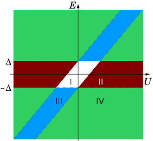
Figure 1: (Color online) Energy domains for the QD states. I (white): no states. II (black, red): bound states. III (gray, blue): tunneling states. IV (light gray, green): scattering states.

In the ’energy vs. potential’ diagram, as shown in Fig. 1, one distinguishes between four different behaviors of the wavefunction. The diagram is symmetric under the transformations $E\to-E$ and $U\to-U$, and can be understood as follows. Everywhere in the diagram, the wavevectors inside and outside the dot satisfy $k^{\prime 2}=(E-U)^{2}-\Delta^{2}$ and $k^{2}=E^{2}-\Delta^{2}$, respectively. In domain I, one has $|E-U|<\Delta$ and $|E|<\Delta$, and consequently $k^{\prime 2}<0$ and $k^{2}<0$. Therefore, both wavevectors $k^{\prime}$ and $k$ are purely imaginary and the wavefunction decays inside and outside the QD. The domain II consists of all the $E$ and $U$ values that satisfy the $|E-U|>\Delta$ and $|E|<\Delta$ inequalities ($k^{\prime 2}>0$ and $k^{2}<0$), so that $k^{\prime}$ is real and $k$ is purely imaginary. True bound states that oscillate for $r<R$ and decay as $\exp{(-r\sqrt{\Delta^{2}-E^{2}})}$ when $r\rightarrow\infty$, can exist therefore only in the energy domain II. For domain III one has $|E-U|<\Delta$ and $|E|>\Delta$, i.e., $k^{\prime 2}<0$ and $k^{2}>0$. Here, the wavevector $k^{\prime}$ is imaginary and $k$ is real, so that the wavefunction decays inside and oscillates outside the QD (tunneling regime). The domain IV is given by $|E-U|>\Delta$ and $|E|>\Delta$, i.e., $k^{\prime 2}>0$ and $k^{2}>0$. Therefore, both $k^{\prime}$ and $k$ are real, and the wavefunction oscillates inside and outside the QD (scattering regime).

In the domain I, the Bessel functions that satisfy the Dirac equation are ${\cal A^{\prime}}_{\pm}I_{J\pm 1/2}(\kappa^{\prime}r)$ for $r<R$ and ${\cal A}_{\pm}K_{J\pm 1/2}(\kappa r)$ for $r>R$. Here, ${\cal A^{\prime}}_{\pm}$ and ${\cal A}_{\pm}$ are the amplitudes of the wavefunction and $\kappa$ and $\kappa^{\prime}$ are the wavevectors inside and outside the QD, respectively. The other two Bessel functions are excluded as possible solutions because they diverge for $r=0$ and $r\rightarrow\infty$, leading to infinite densities at the origin and non-normalizable wavefunctions. The amplitudes are determined from the Dirac equation and from the matching conditions at $r=R$ for the wavefunctions inside and outside the QD. The matching condition leads to an equation for ${\cal A^{\prime}}_{\pm}$ and ${\cal A}_{\pm}$ that has no nonzero real solutions for $\kappa$ and $\kappa^{\prime}$, and hence, there can be no states that decay inside and outside the QD. In the following sections, we discuss the domains II–IV.

II.2 Lattice model

The single band TB Hamiltonian that describes the non-interacting electrons in graphene in the presence of a radially symmetric potential reads

$$\hat{H}_{\text{TB}}=\sum_{\mathbf{r}}(U_{\mathbf{r}}+\Delta_{\mathbf{r}})c_{\mathbf{r}}^{{\dagger}}c_{\mathbf{r}}-t\sum_{\left<\mathbf{r}\neq\mathbf{r}^{\prime}\right>}c_{\mathbf{r}}^{{\dagger}}c_{\mathbf{r}^{\prime}}.$$ (3)

Here, $c_{\mathbf{r}}^{{\dagger}}$ and $c_{\mathbf{r}}$ are the fermionic particle creation and annihilation operators at the sites $\mathbf{r}$ of a hexagonal lattice with carbon-carbon distance $a$. The $\left<\mathbf{r}\neq\mathbf{r}^{\prime}\right>$ denote nearest-neighbor sites and $t=2.7$ eV is the hopping parameter. In the following, we set the energy scale by putting $t=1$. The potential is $U_{\mathbf{r}}=U$ for sites inside the QD ($r<R$) and $U_{\mathbf{r}}=0$ outside. Also, we have introduced a lattice anisotropy $\Delta_{\mathbf{r}}$ for the two sublattices of graphene, $\Delta_{\pm}=\pm\Delta$. This anisotropy opens an energy gap $2\Delta$ in the spectrum and allows for the existence of true bound states. In the presence of disorder to be considered later, the above Hamiltonian is modified to account also for random on-site potentials or for random transfer terms between nearest neighbor sites.

III Bound states of the isolated QD

III.1 Continuum model

In this section, the energies of the bound states are calculated. To this end, we put $V(r)=U\Theta(R-r)$ and consider the region II in Fig. 1. The solution of the radial Dirac equation for $r\gtrless R$ is given in terms of Bessel functions as

$$\xi_{\pm}(r)=\left\{\begin{array}[]{ll}{{\cal A}}^{\prime}_{\pm}\,J_{J\pm\frac{1}{2}}(k^{\prime}r),&r<R\\ {{\cal A}}_{\pm}\,K_{J\pm\frac{1}{2}}(\kappa r),&r>R.\end{array}\right.$$ (4)

The other two Bessel functions are excluded as solutions: for $r\to 0$, $N_{J\pm\frac{1}{2}}(k^{\prime}r)$ diverges and the density would be infinite at the origin, for large $r$, $I_{J\pm\frac{1}{2}}(\kappa r)$ diverges and the wavefunction would not be normalizable. The amplitudes ${{\cal A}}_{-}$ and ${{\cal A}}^{\prime}_{-}$ are tied to ${{\cal A}}_{+}$ and ${{\cal A}}^{\prime}_{+}$, respectively, by the equations of motion

$$\begin{array}[]{rl}\left(\begin{array}[]{cc}E-U-\Delta&-ik^{\prime}\\ ik^{\prime}&E-U+\Delta\end{array}\right)\left(\begin{array}[]{c}{{\cal A}}^{\prime}_{+}\\ {{\cal A}}^{\prime}_{-}\end{array}\right)=0,&r<R\\ \left(\begin{array}[]{cc}E-\Delta&-i\kappa\\ -i\kappa&E+\Delta\end{array}\right)\left(\begin{array}[]{c}{{\cal A}}_{+}\\ {{\cal A}}_{-}\end{array}\right)=0,&r>R.\end{array}$$ (5)

There are two matching conditions at $r=R$. Thus one obtains the following condition for the existence of a non-zero wavefunction (bound state)

$$\sqrt{\frac{E-U+\Delta}{E-U-\Delta}}\;\frac{J_{J+\frac{1}{2}}(k^{\prime}R)}{J_{J-\frac{1}{2}}(k^{\prime}R)}=-\sqrt{\frac{\Delta+E}{\Delta-E}}\;\frac{K_{J+\frac{1}{2}}(\kappa R)}{K_{J-\frac{1}{2}}(\kappa R)}.$$ (6)

The other valley yields a corresponding equation with $(J+1/2)$ replaced by $-(J-1/2)$. Since we have to consider all half-integer $J$’s in Eq. (6), each bound state is doubly degenerate when one considers both valleys. In Fig. 2, we show the evaluation of the energies of the bound states vs. the QD radius and vs. the value of the potential. Since everything is symmetric under $E\to-E$ and $U\to-U$ as mentioned above, we show only states for $U\geq 0$. For clarity, we present only the states with $J=1/2$, $3/2$, and $5/2$. Here, we use $\Delta=0.1$ in TB units $t=1$ (which corresponds to $\Delta=0.27$ eV). Note that when $R=25\,a$ and $U=0.2$, there are six bound states in the QD: three with $J=1/2$, two with $J=3/2$, and only one with $J=5/2$, as shown in Fig. 2. When the QD radius or the strength of the confinement potential increases, more bound states can be accommodated in the QD. Our results are in excellent agreement with previous calculations of bound state energies in a radially-symmetricRecher et al. (2009) or a rectangular-shapedTrauzettel et al. (2007) graphene QD.

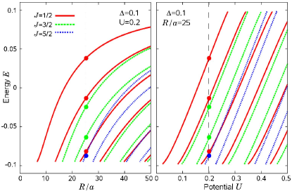
Figure 2: (Color online) The energies of the bound states in a graphene QD as function of the dot radius (left panel) and potential strength (right panel). We use $\Delta=0.1$ and show the results for $J=1/2$ (solid line), $J=3/2$ (dashed line), and $J=5/2$ (dotted line) only. The intersections of the solutions with the vertical lines yield the bound states energies for $R=25\,a$ and $U=0.2$.

III.2 Lattice model

It is well known that the above results obtained within the commonly applied continuum Dirac-fermion approximation have a limited range of validity. To investigate this in more detail and to check possible deviations originating from neglecting lattice effects, we compute the eigenvalues of the lattice model via a numerical diagonalization of the TB Hamiltonian (3). In our calculations, we study a graphene ribbon consisting of $2N_{\rm ac}\times N_{\rm zz}=2\cdot 100\times 100$ carbon atoms with periodic boundary conditions ($N_{\rm ac}$ and $N_{\rm zz}$ are the number of armchair and zigzag lines, respectively). For the lattice anisotropy, we take $\Delta_{\pm}=\pm 0.1$ and calculate the eigenvalues for several QD radii as a function of the potential strength. Changing $N_{\rm ac}$ or $N_{\rm zz}$ does not alter the resulting eigenenergies $E$ between $-\Delta$ and $\Delta$ as long as $N_{\rm ac}a\approx N_{\rm zz}a\gg R\gg a$.

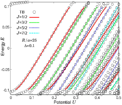
Figure 3: (Color online) Comparison between the eigenenergies of the TB Hamiltonian (circles) of the graphene lattice and the solutions of the Dirac equation (lines) as a function of the potential $U$. The parameters used are $\Delta=0.1$ and $R=25\,a$.

Figure 3 exhibits the eigenvalues of the TB Hamiltonian (3) vs. the potential $U$ in the energy range $|E|<\Delta$. For comparison, we show also the eigenenergy solutions of the Dirac equation for the bound states as given by Eq. (6). We restrict the angular momentum to $J\leq 7/2$ for the sake of clarity. There is an excellent agreement between the two approaches for small angular momenta and small $U$. The angular momentum is not a good quantum number in the lattice model, nevertheless, we can identify the energies in both models for small angular momenta. If larger QD radii are considered, the good agreement between the TB and the Dirac equation becomes better even for higher values of $J$ (results not shown here because there are too many eigenvalues in the figure, already for $R\sim 60\,a$). The reason for the slight deviations for small QD radii are the irregularities at the QD border appearing in the lattice model but which are not present in the continuum model. The corresponding lattice QD is not a perfect circle but has a chiseled edge.

IV Transport properties of a graphene QD

IV.1 Continuum model

In this section, we want to calculate the transport properties through the circular QD. For this purpose, we need to introduce an environment to the isolated QD so that the exponentially decaying bound states are still finite when reaching the outer region. We take a radially symmetric model with the following potential

$$V(r)=\left\{\begin{array}[]{ll}U,&0<r<R\\ 0,&R<r<L\\ V,&L<r\end{array}\right..$$ (7)

The profile of the potential, which now consists of three regions, is schematically shown in Fig. 4. The radially symmetric choice makes the analytic determination of the S-matrix possible. Next, we explain our setup and sketch the derivation of the S-matrix.

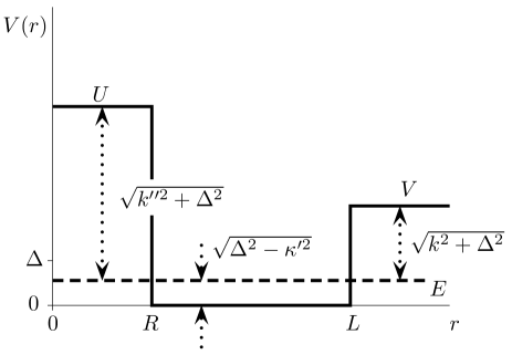
Figure 4: (Color online) Potential landscape of a QD with radius $R$ and an additional environment for $r>L$. The vertical dotted arrows indicate $|E-V(r)|$ in each of the three regions. For $R<r<L$, the wavefunctions decay. Also, $k^{\prime\prime}$, $k^{\prime}=i\kappa^{\prime}$, and $k$ are the wavevectors inside the QD, outside, and in the environment region, respectively.

Compared to the isolated QD, there is a third region for the radial component, $r>L$. Here, the potential $V$ is chosen such that the wavefunctions are oscillatory. Then, we can have incoming and outgoing waves in the environment and define a scattering cross-section. In the intermediate region, $R<r<L$, the wave functions decay, and inside the QD, $0<r<R$, the energy can belong to bound states. This corresponds to the regime II of the isolated QD.

Next, we turn to the definition of the scattering matrix ${\cal S}$.Novikov (2007); Katsnelson and Novoselov (2007); Guinea (2008). For $r\to\infty$, we write the wave function as

$$\xi_{\pm}({\mathbf{x}}) = \frac{1}{\sqrt{2}}\sqrt{E-V\pm\Delta}\;e^{ikx}+$$ (8)

$$\frac{1}{\sqrt{2\pi kr}}\sqrt{E-V\pm\Delta}\;f_{\pm}(\varphi)\;e^{ikr}.$$

The first term is the incoming plane wave in $x$ direction, the second the outgoing spherical wave. Furthermore, $f_{\pm}(\varphi)$ is the scattering amplitude, with $f_{+}(\varphi)=e^{i\varphi}f_{-}(\varphi)$, and $\varphi$ is the scattering angle. The two components of $\xi$ individually solve the Dirac equation for graphene and are normalized such that the incoming (plane wave) particle current density is $k$, while the number of particles leaving per unit time radially in the direction $\varphi$ is $d\varphi\frac{1}{2\pi}\left(f_{+}^{*}(\varphi)e^{i\varphi}f_{-}(\varphi)+f_{-}^{*}(\varphi)e^{-i\varphi}f_{+}(\varphi)\right)$. Thus, the differential scattering cross section is

$$\frac{d\sigma(\varphi)}{d\varphi}=\frac{1}{2\pi k}\left(f_{+}^{*}(\varphi)e^{i\varphi}f_{-}(\varphi)+f_{-}^{*}(\varphi)e^{-i\varphi}f_{+}(\varphi)\right).$$ (9)

We then expand in angular momenta with coefficients $f_{J}$

$$f_{\pm}(\varphi)=\frac{1}{\sqrt{2}}\sum_{J}e^{i\varphi(J\pm\frac{1}{2})-i\frac{\pi}{4}}\;f_{J}$$ (10)

and define the scattering matrix ${\cal S}_{J}$ as ${\cal S}_{J}=1+f_{J}$ to obtain

$$\frac{d\sigma(\varphi)}{d\varphi}=\frac{1}{2\pi k}\sum_{J,J^{\prime}}\;e^{i\varphi(J-J^{\prime})}\;({{\cal S}}_{J^{\prime}}^{*}-1)({\cal S}_{J}-1)\;.$$ (11)

Next we sketch the calculation of ${\cal S}_{J}$. In our geometry, the general solution of the Dirac equation for fixed angular momentum $J$ is given by

$$\xi_{\pm}(r)=$$

$$\left\{\begin{array}[]{ll}{{\cal A}}_{\pm}\;H^{(1)}_{J\pm\frac{1}{2}}(kr)+{{\cal B}}_{\pm}\;H^{(2)}_{J\pm\frac{1}{2}}(kr),&L<r\\ {{\cal A}}^{\prime}_{\pm}\;K_{J\pm\frac{1}{2}}(\kappa^{\prime}r)+{{\cal B}}^{\prime}_{\pm}\;I_{J\pm\frac{1}{2}}(\kappa^{\prime}r),&R<r<L\\ {{\cal A}}^{\prime\prime}_{\pm}\;J_{J\pm\frac{1}{2}}(k^{\prime\prime}r),&r<R.\end{array}\right.$$

Here, the wave vectors are $k=\sqrt{(E-V)^{2}-\Delta^{2}}$, $\kappa^{\prime}=\sqrt{\Delta^{2}-E^{2}}$, and $k^{\prime\prime}=\sqrt{(E-U)^{2}-\Delta^{2}}$. Using in (8)

$$e^{ikr\cos(\varphi)}=\sum_{m=-\infty}^{\infty}e^{i(\varphi+\frac{1}{2}\pi)m}\;J_{m}(kr)\;,$$ (13)

we can easily find the expression for ${{\cal A}}_{\pm}$ and ${{\cal B}}_{\pm}$ from the ansatz Eq. (8), i.e., the relation between ${{\cal A}}_{\pm}$ and ${{\cal B}}_{\pm}$ and ${\cal S}_{J}$. Then, ${{\cal A}}_{\pm}$ and ${{\cal B}}_{\pm}$ are related to ${{\cal A}}^{\prime}_{\pm}$ and ${{\cal B}}^{\prime}_{\pm}$, and these in turn to ${{\cal A}}^{\prime\prime}_{\pm}$ by the matching conditions. Thus, the elements of the scattering matrix ${\cal S}_{J}$ are determined. We skip the tedious but straight-forward (linear) algebra and just quote the result

$${\cal S}_{J}=-\frac{\det{\cal D}^{(2)}}{\det{\cal D}^{(1)}}$$ (14)

and

$${\cal D}^{(1,2)}=$$

$${\left(\begin{array}[]{cccc}0&w^{\prime}_{+}K_{J_{+}}(x^{\prime}_{R})&w^{\prime}_{+}I_{J_{+}}(x^{\prime}_{R})&w^{\prime\prime}_{+}J_{J_{+}}(x^{\prime\prime})\\ 0&w^{\prime}_{-}K_{J_{-}}(x^{\prime}_{R})&-w^{\prime}_{-}I_{J_{-}}(x^{\prime}_{R})&w^{\prime\prime}_{-}J_{J_{-}}(x^{\prime\prime})\\ w_{+}H^{(2,1)}_{J_{+}}(x)&w^{\prime}_{+}K_{J_{+}}(x^{\prime}_{L})&w^{\prime}_{+}I_{J_{+}}(x^{\prime}_{L})&0\\ w_{-}H^{(2,1)}_{J_{-}}(x)&w^{\prime}_{-}K_{J_{-}}(x^{\prime}_{L})&-w^{\prime}_{-}I_{J_{-}}(x^{\prime}_{L})&0\end{array}\right)}$$ (19)

(20)

The appearance of the determinants is easily explained: they result from the solution of the $4$ linear matching conditions ($2$ for $\xi_{\pm}$ at $r=L$ and $2$ more at $r=R$). Again, $H^{(1,2)}_{m}(x)$, $K_{m}(x)$, $I_{m}(x)$, and $J_{m}(x)$ are the standard Bessel functions and we use the following abbreviations:

$$w_{\pm}:=\sqrt{|E-V\pm\Delta|}\;,\quad w^{\prime\prime}_{\pm}:=\sqrt{|E-U\pm\Delta|}\;,\quad$$

$$w^{\prime}_{\pm}:=\sqrt{|E\pm\Delta|}\;,\quad J_{\pm}:=J\pm\frac{1}{2}\;,$$

$$x:=kL,\quad x^{\prime}_{R;L}:=\kappa^{\prime}R;\ \kappa^{\prime}L\;,\quad x^{\prime\prime}:=k^{\prime\prime}R\;.$$ (21)

To make connection with the two-terminal conductance that can be measured in experiments, we calculate the transport cross section asKatsnelson et al. (2009)

$$\sigma_{tr}:=\int_{-\pi}^{\pi}d\varphi\;(1-\cos\varphi)\;\frac{d\sigma(\varphi)}{d\varphi}.$$ (22)

For the scattering cross section from Eq. (11) we use the ${\cal S}_{J}$ computed according to Eqs. (14-IV.1). The results are shown in Fig. 5, where we compare the bound state energies of an isolated graphene QD of fixed size $R$ and for fixed potential $U$ with the positions of the resonances in the transport cross section of the QD plus environment. The bound state energies and the positions of the resonances exactly coincide. When the energy of an incoming particle matches that of a bound state, the particle tunnels through the QD and the cross section is small. The ’background’ cross-section is given by $\sigma_{tr}(U=0)$, i.e., by the cross section of an ’empty’ QD.

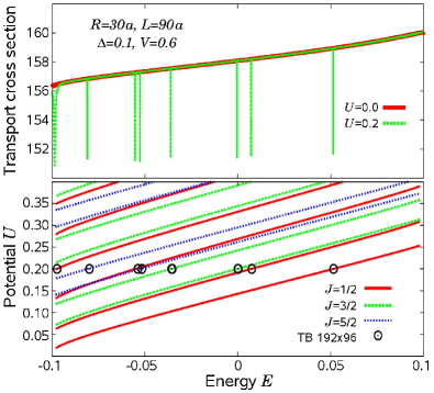
Figure 5: (Color online) Transport cross-section of a graphene quantum dot ($R/a=30$, $\Delta=\pm 0.1$) with environment (upper panel). The position of the peaks correspond to the energies of the bound states of an isolated graphene QD with dot potential $U=0.2$. They also agree with the results from the corresponding TB model (circles in the lower panel). The transport cross section (green dotted line) is shown in arbitrary units with the ’background’ value (red solid line) given by the empty dot $U=0$.

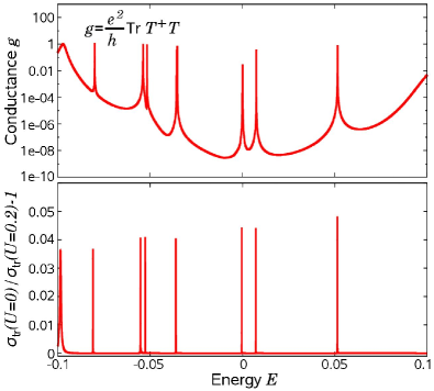
Figure 6: (Color online) The two-terminal conductance $g$ (upper panel) calculated within a TB model compared to the normalized transport cross section (lower panel) of a continuum Dirac model.

IV.2 Lattice model

In this subsection, the two-terminal conductance $g$ through a graphene quantum dot is calculated numerically within a lattice model and compared with the results of the transport cross-section of the continuum model. The two-terminal conductanceEconomou and Soukoulis (1981) is obtained from the transmission matrix $T$ employing the transfer-matrix methodPendry et al. (1992) according to

$$g=\frac{e^{2}}{h}{\text{Tr}}\,T^{{\dagger}}T=\frac{e^{2}}{h}\sum_{i}^{N}(\cosh^{2}(\varepsilon_{i}/2))^{-1},$$ (23)

where the $\varepsilon_{i}$ parameterize the eigenvalues of $T$, and $N$ is the number of open channels. The electron transmission through a sample of width $L_{y}=96\,a$ and length $L_{x}=192\,a$ with two semi-infinite leads attached at $x=1$ and $x=L_{x}$ is calculated numerically. Periodic boundary conditions are applied in the $y$ direction. The sublattice anisotropy, the dot potential and radius are $\Delta/t=\pm 0.1$, $U/t=0.2$, and $R/a=30$, respectively. The outcome is shown in Fig. 6, where the two-terminal conductance (upper panel) and the relative transport cross-section (lower panel) are plotted as a function of energy. The latter is normalized according to $\sigma_{tr}(U=0)/\sigma_{tr}(U)-1$ while the former is displayed on a log-scale in order to make the comparison easier. The reason is that in contrast to the transport cross-section of the infinite system considered in the continuum model, the two-terminal conductance, due to the finite sample length in the lattice model, does not drop to zero between the resonances that are associated with the bound states. For the energetic positions of the resonances, an excellent agreement is obtained between the two approaches. However, the agreement between the two is good only as long as $R\gg a$. When the QD radius is reduced, the positions of the transport peaks, calculated within the continuum model, differ from those of the lattice model due to the irregularities at the QD edges appearing in the latter approach.

It is clear that the electrostatic potential confining the QD cannot be infinitely steep in real samples. Therefore, we also studied the effect of linearly sloping dot potential steps. We find that the electronic bound states of the QD shift linearly to smaller energies when the slope of the QD walls decreases. Therefore, it can happen that the bound states’ energies fall below the lower edge of the gap, $E=-\Delta$. Hence, in experiments the dot potentials should be fabricated as steeply as possible.

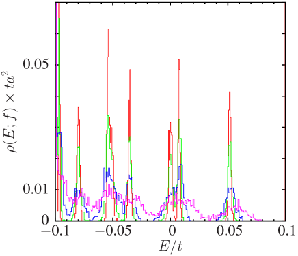
Figure 7: (Color online) Influence of random magnetic flux disorder on the density of states of a circular QD with radius 30 $a$ and dot potential $U/t=0.2$. The sublattice difference is $\Delta/t=\pm 0.1$ as before. With increasing disorder, $f/(h/e)=\mathrm{0.005}$ (red), 0.01 (green), 0.02 (blue), and 0.05 (magenta), the peaks get broadened and start to overlap.

V Influence of disorder

Real graphene samples are usually subject to various disturbances and imperfections. It is known that the electronic properties essentially depend on the particular type of disorder present. In the following, we study the influence of possible modifications that may affect the bound states of an electrostatically confined graphene quantum dot. The lattice model Hamiltonian of the unperturbed system (3) is now modified to allow for diagonal and non-diagonal disorder. The latter arises in graphene when either ripples or random magnetic fields are present.Morozov et al. (2006); Morpurgo and Guinea (2006); Meyer et al. (2007); Guinea et al. (2008); Schweitzer and Markoš (2008) The impact of random on-site disorder that can be due to adsorbed atoms and molecules attached to the bulk or to the dangling bonds along the edges of the graphene sheet, is described by diagonal random disorder potentials

$${\cal H}=\sum_{\mathbf{r}}(U_{\mathbf{r}}+\Delta_{\mathbf{r}}+\epsilon_{\mathbf{r}})\,c_{\mathbf{r}}^{\dagger}c_{\mathbf{r}}-t\sum_{\langle\mathbf{r}\neq\mathbf{r}^{\prime}\rangle}e^{-i\theta_{\mathbf{r}\mathbf{r}^{\prime}}}c_{\mathbf{r}}^{\dagger}c_{\mathbf{r}^{\prime}}.$$ (24)

Again, $t=2.7$ eV is the nearest-neighbor transfer energy for graphene, $\mathbf{r}$ denotes the sites of the carbon atoms, and $\langle\mathbf{r}\neq\mathbf{r}^{\prime}\rangle$ are pairs of those neighboring sites on a bricklayer latticeSchweitzer and Markoš (2008) that are connected by bonds. The sample width and the length are $L_{y}=96\,a$ and $L_{x}=192\,a$, respectively. Periodic boundary conditions (BC) are applied in the $x$ direction (length) and Dirichlet BC in the $y$ direction (width). As before, $U_{\mathbf{r}}$ and $\Delta_{\mathbf{r}}$ define the quantum dot potential and the sub-lattice anisotropy, respectively. The on-site potentials $\epsilon_{\mathbf{r}}$ describe either the uncorrelated random bulk disorder or the one-dimensional edge-disorder. A box-probability distribution $P(\epsilon_{\mathbf{r}})=1/W$ is assumed for the random potentials $-W/2\leq\epsilon_{\mathbf{r}}\leq W/2$, where $W$ is a measure of the disorder strength. The case of ripples and corrugations is modeled by an equivalent random-magnetic-flux (RMF) disorder model leading to complex phase factors that are defined by $\sum\theta_{\mathbf{r}\mathbf{r}^{\prime}}=2\pi e\phi_{\mathbf{r}}/h$, where the sum is taken along the bonds around a given plaquette situated at $\mathbf{r}$ with the random flux $\phi_{\mathbf{r}}$ piercing through it. Without a QD, the chiral symmetry is conservedOstrovsky et al. (2006); Markoš and Schweitzer (2007); Schweitzer and Markoš (2008); Schweitzer (2009) in this disorder model. The random fluxes are also drawn at random from a box distribution $-f/2\leq\phi_{\mathbf{r}}\leq f/2$ with zero mean, and $h/e$ is the magnetic flux quantum. The RMF-disorder strength $f$ varies between $0\leq f/(h/e)\leq 1$.

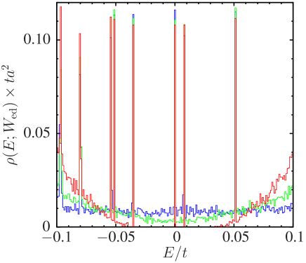
Figure 8: (Color online) The density of states $\rho(E;W_{\rm ed})$ within the gap arising from the sublattice difference $\Delta/t=\pm 0.1$ in the presence of edge disorder of strengths $W_{\rm ed}/t=\mathrm{0.1}$ (red), 0.2 (green), and 0.5 (blue). The bound states energies of the quantum dot (radius 30 $a$, potential strength 0.2 $t$) remain almost unaffected by the edge disorder.

The result of random-flux disorder is shown in Fig. 7, where the density of states (DOS) of a graphene sheet with quantum dot and sublattice anisotropy is plotted for energies around the Dirac point. The sublattice difference is taken to be $\Delta/t=\pm 0.1$, the quantum dot potential is $U/t=0.2$, and the QD radius is $R/a=30$. The peaks of the bound states are still clearly visible in the case of small disorder strength $f/(h/e)=0.005$. With increasing disorder, however, the peaks get broadened and disappear for $f/(h/e)=0.05$. Therefore, the sharp bound energy states of a clean graphene QD can be destroyed in the presence of sufficiently strong ripple disorder.

A completely different behavior is obtained in the case of one-dimensional edge-disorder only.Evaldsson et al. (2008); Mucciolo et al. (2009); Kunstmann et al. (2011) This can be seen in Fig. 8 where again the DOS is shown for energies within the gap $\Delta/t=\pm 0.1$ of a quantum dot with potential $U/t=0.2$. With increasing edge-disorder strength from $W_{\rm ed}/t=0.0$ to $W_{\rm ed}/t=0.5$, only the DOS of the peaks lying outside the gap are broadened and eventually completely fill the energy regions between the sharp bound states that remain unaffected. Hence, electrostatically confined graphene QD do not deteriorate in the presence of edge-disorder and remain suited for experimental spectroscopic studies. This behavior is due to the exponential decay of the edge states which do not get mixed with the localized bound states of the QD even in the presence of additional edge-disorder potentials.

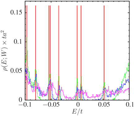
Figure 9: (Color online) The density of states $\rho(E;W)$ showing the bound states of the quantum dot (radius 30 $a$, potential strength 0.2 $t$) within the gap arising from the sublattice difference $\Delta/t=\pm 0.1$ in the presence of on-site disorder of strengths $W/t=\mathrm{0.0}$ (red), 0.05 (green), 0.1 (blue), and 0.2 (magenta). The sharp DOS-peaks broaden and finally disappear with increasing disorder strength.

When in addition to edge disorder the random on-site potentials are also allowed to affect the bulk sites, the DOS of the quantum dot’s bound states get broadened with increasing disorder strength as can be seen in Fig. 9. As in the case of the random-flux disorder, but in stark contrast to the edge-disorder only situation, the sharp peaks broaden and finally disappear for disorder strength $W/t>0.2$. A similar behavior is seen in the two-terminal conductance where, with increasing disorder strength, the single sharp resonances are replaced by a cluster of resonances which essentially depend on the particular disorder realization. So, uncorrelated short-range random potentials of sufficient strength destroy the discreteness of the QD energies. In order to fabricate electrostatically defined graphene quantum dots, only samples that are clean, at least in the bulk area, can be used, whereas disorder at the edges is of minor importance.

VI Conclusions

The electronic properties of circular graphene quantum dots, which can be created electrostatically in the presence of a sublattice asymmetry, were investigated with the aid of two different models. First, we used a continuum model described by a Dirac-type equation that can be solved analytically, and second, we applied a tight-binding lattice model, which was evaluated numerically. The dependence of the electronic bound states and the transport cross-section on the electrostatic potential and size of the quantum dot were calculated. Both the spectra of bound quantum dot states and the electric transport through the QD show a very good agreement between the two models when the radius of the QD is much larger than the carbon-carbon distance $a$. For smaller dot radii, the agreement is always reasonable for the low lying bound states, but gets worse at higher energies where in the continuum model the large angular momenta essentially contribute. In experiments, QDs of sizes 20–50 nm are fabricatedPonomarenko et al. (2008); Todd et al. (2009); Güttinger et al. (2009) which means $R/a\approx 70-176$. For such radii, the agreement between the two models is very good even for bound states with high values of the angular momentum $J$.

The results of the transport cross-section for a QD with attached environment calculated within the infinite continuum model coincided with the numerically evaluated two-terminal conductance obtained for a finite graphene sample with attached semi-infinite leads described by a tight-binding lattice model. Within the TB model, we also studied the influence of a sloping dot potential, which caused the energy levels to shift to lower energies, and of bulk and edge disorder on the bound states of electrostatically defined graphene quantum dots.

The presence of disorder severely influences the quantum dot’s spectral and transport properties. Only in the case of one-dimensional uncorrelated random edge-disorder, do the peaks of the density of states corresponding to the bound states remain sharp. For on-site or random-magnetic-flux (ripple) bulk disorder, the peaks of the bound states in the DOS are broadened and finally disappear with increasing disorder strength, and thus the quantum dot loses its experimentally observable characteristic spectral fingerprint.

References

- Han et al. (2007) M. Y. Han, B. Özyilmaz, Y. Zhang, and P. Kim, Phys. Rev. Lett. 98, 206805 (2007).
- Li et al. (2008) X. Li, X. Wang, L. Zhang, S. Lee, and H. Dai, Science 319, 1229 (2008).
- Ponomarenko et al. (2008) L. A. Ponomarenko, F. Schedin, M. I. Katsnelson, R. Yang, E. W. Hill, K. S. Novoselov, and A. K. Geim, Science 320, 356 (2008).
- Stampfer et al. (2008) C. Stampfer, E. Schurtenberger, F. Molitor, J. Güttinger, T. Ihn, and K. Ensslin, Nanoletters 8, 2378 (2008).
- Todd et al. (2009) K. Todd, H.-T. Chou, S. Amasha, and D. Goldhaber-Gordon, Nano Letters 9, 416 (2009).
- Güttinger et al. (2009) J. Güttinger, C. Stampfer, F. Libisch, T. Frey, J. Burgdörfer, T. Ihn, and K. Ensslin, Phys. Rev. Lett. 103, 046810 (2009).
- Libisch et al. (2010) F. Libisch, S. Rotter, J. Güttinger, C. Stampfer, and J. Burgdörfer, Phys. Rev. B 81, 245411 (2010).
- Katsnelson et al. (2006) M. I. Katsnelson, K. S. Novoselov, and A. K. Geim, Nature Physics 2, 620 (2006).
- Pereira Jr et al. (2010) J. M. Pereira Jr, F. M. Peeters, A. Chaves, and G. A. Farias, Semicond. Sci. Technol. 25, 033002 (2010).
- Huard et al. (2007) B. Huard, J. A. Sulpizio, N. Stander, K. Todd, B. Yang, and D. Goldhaber-Gordon, Phys. Rev. Lett. 98, 236803 (2007).
- Stander et al. (2009) N. Stander, B. Huard, and D. Goldhaber-Gordon, Phys. Rev. Lett. 102, 026807 (2009).
- Young and Kim (2009) A. F. Young and P. Kim, Nature Physics 5, 222 (2009).
- Velasco Jr et al. (2009) J. Velasco Jr, G. Liu, W. Bao, and C. N. Lau, New J. Phys. 11, 095008 (2009).
- Son et al. (2006) Y.-W. Son, M. L. Cohen, and S. G. Louie, Phys. Rev. Lett. 97, 216803 (2006).
- Apel et al. (2011) W. Apel, G. Pal, and L. Schweitzer, Phys. Rev. B 83, 125431 (2011).
- Gui et al. (2008) G. Gui, J. Li, and J. Zhong, Phys. Rev. B 78, 075435 (2008).
- Pereira et al. (2009) V. M. Pereira, A. H. Castro Neto, and N. M. R. Peres, Phys. Rev. B 80, 045401 (2009).
- Giovannetti et al. (2007) G. Giovannetti, P. A. Khomyakov, G. Brocks, P. J. Kelly, and J. van den Brink, Phys. Rev. B 76, 073103 (2007).
- Ribeiro et al. (2008) R. M. Ribeiro, N. M. R. Peres, J. Coutinho, and P. R. Briddon, Phys. Rev. B 78, 075442 (2008).
- Zhou et al. (2007) S. Y. Zhou, G.-H. Gweon, A. V. Fedorov, P. N. First, W. A. de Heer, D.-H. Lee, F. Guinea, A. H. Castro Neto, and A. Lanzara, Nat. Mater. 6, 770 (2007).
- Silvestrov and Efetov (2007) P. G. Silvestrov and K. B. Efetov, Phys. Rev. Lett. 98, 016802 (2007).
- Matulis and Peeters (2008) A. Matulis and F. M. Peeters, Phys. Rev. B 77, 115423 (2008).
- Hewageegana and Apalkov (2008) P. Hewageegana and V. Apalkov, Phys. Rev. B 77, 245426 (2008).
- Bardarson et al. (2009) J. H. Bardarson, M. Titov, and P. W. Brouwer, Phys. Rev. Lett. 102, 226803 (2009).
- Trauzettel et al. (2007) B. Trauzettel, D. V. Bulaev, D. Loss, and G. Burkhard, Nature Physics 3, 192 (2007).
- Recher et al. (2009) P. Recher, J. Nilsson, G. Burkard, and B. Trauzettel, Phys. Rev. B 79, 085407 (2009).
- Schnez et al. (2008) S. Schnez, K. Ensslin, M. Sigrist, and T. Ihn, Phys. Rev. B 78, 195427 (2008).
- Wassmann et al. (2008) T. Wassmann, A. P. Seitsonen, A. M. Saitta, M. Lazzeri, and F. Mauri, Phys. Rev. Lett. 101, 096402 (2008).
- Bostwick et al. (2009) A. Bostwick, J. L. McChesney, K. V. Emtsev, T. Seyller, K. Horn, S. D. Kevan, and E. Rotenberg, Phys. Rev. Lett. 103, 056404 (2009).
- Morozov et al. (2006) S. V. Morozov, K. S. Novoselov, M. I. Katsnelson, F. Schedin, L. A. Ponomarenko, D. Jiang, and A. K. Geim, Phys. Rev. Lett. 97, 016801 (2006).
- Morpurgo and Guinea (2006) A. F. Morpurgo and F. Guinea, Phys. Rev. Lett. 97, 196804 (2006).
- Meyer et al. (2007) J. C. Meyer, A. K. Geim, M. I. Katsnelson, K. S. Novoselov, T. J. Booth, and S. Roth, Nature 446, 60 (2007).
- Guinea et al. (2008) F. Guinea, M. I. Katsnelson, and M. A. H. Vozmediano, Phys. Rev. B 77, 075422 (2008).
- Wimmer et al. (2010) M. Wimmer, A. R. Akhmerov, and F. Guinea, Phys. Rev. B 82, 045409 (2010).
- Katsnelson and Novoselov (2007) M. Katsnelson and K. Novoselov, Solid State Communications 143, 3 (2007).
- Guinea (2008) F. Guinea, J. Low Temp. Phys. 153, 359 (2008).
- Novikov (2007) D. S. Novikov, Phys. Rev. B 76, 245435 (2007).
- Katsnelson et al. (2009) M. I. Katsnelson, F. Guinea, and A. K. Geim, Phys. Rev. B 79, 195426 (2009).
- Economou and Soukoulis (1981) E. N. Economou and C. M. Soukoulis, Phys. Rev. Lett. 46, 618 (1981).
- Pendry et al. (1992) J. B. Pendry, A. MacKinnon, and P. J. Roberts, Proc. R. Soc. London A 437, 67 (1992).
- Schweitzer and Markoš (2008) L. Schweitzer and P. Markoš, Phys. Rev. B 78, 205419 (2008).
- Ostrovsky et al. (2006) P. M. Ostrovsky, I. V. Gornyi, and A. D. Mirlin, Phys. Rev. B 74, 235443 (2006).
- Markoš and Schweitzer (2007) P. Markoš and L. Schweitzer, Phys. Rev. B 76, 115318 (2007).
- Schweitzer (2009) L. Schweitzer, Phys. Rev. B 80, 245430 (2009).
- Evaldsson et al. (2008) M. Evaldsson, I. V. Zozoulenko, H. Xu, and T. Heinzel, Phys. Rev. B 78, 161407 (2008).
- Mucciolo et al. (2009) E. R. Mucciolo, A. H. Castro Neto, and C. H. Lewenkopf, Phys. Rev. B 79, 075407 (2009).
- Kunstmann et al. (2011) J. Kunstmann, C. Özdoğan, A. Quandt, and H. Fehske, Phys. Rev. B 83, 045414 (2011).