Non-Markovian dynamics of system-reservoir entanglement

Abstract

Using an exact approach, we study the dynamics of entanglement between two qubits coupled to independent reservoirs and between the two, initially disentangled, reservoirs. We also describe the transfer of bipartite entanglement from the two-qubits to their respective reservoirs focussing on the case of two atoms inside two different leaky cavities with a specific attention to the role of the detuning. We present a scheme to prepare the cavity fields in a maximally entangled state, without direct interaction between the cavities, by exploiting the initial qubits entanglement. We discuss a deterministic protocol, working in the presence of cavity losses, for the generation of a W-state of one qubit and two cavity fields and we describe a probabilistic scheme to entangle one of the atoms with the reservoir (cavity field) of the other atom.

1 Introduction

The decoherence of entangled systems has been the subject of an intense research activity in the last few years, triggered by the theoretical prediction of the phenomenon of entanglement sudden death (ESD) [1], experimentally demonstrated with entangled photon pairs [2] and atomic ensembles [3]. Subsequent theoretical paper have extended the original work in various directions, by studying the dynamics of entangled systems coupled to either the same [4] or different reservoirs, including non-markovian effects [5] experimentally tested in [6]; by examining the effect of finite temperature reservoirs [7]; by including counter-rotating terms [8] and by exploring the role of diversity between the subsystems [9, 10]. Furthermore, it has been understood that the sudden death phenomenon is, in fact, rather a transfer, as the environmental degrees of freedom become entangled while the two subsystems disentangle [11] (entanglement sudden birth, ESB).

The study of reservoirs entanglement in relationship to the phenomenon of entanglement sudden death has been also performed for two-level-systems interacting with two ideal cavities [12, 13]. Further investigations have been devoted to the existence of entanglement invariant [14].

The first aim of this paper is to study the sudden birth phenomenon in the case of non-markovian reservoirs, in order to elucidate the role of entanglement memory on entanglement exchange. In doing this, we will show that the two cases of i)a spectrally flat, markovian environment, and of ii)a monochromatic environment, first studied in Refs. [11] and [12], respectively, are just two manifestation of the same phenomenon, as both of them can be described in a unique fashion (see also Ref. [15]). Indeed, the Hamiltonian model that we discuss continuously interpolates between these two extrema depending on the spectral width of the environmental projected density of states.

More explicitly, we present an exact approach to the dynamics of two qubits interacting with independent structured reservoirs having Lorentzian spectral distributions. This system describes, e.g., two atoms inside two leaky cavities, whose quality factors are related to the widths of the Lorentzians, and provides a quite realistic description of the case of two ions trapped into two cavities, as discussed in Ref. [16]. The solution of this model reduces to the Markovian one in the bad cavity limit and to the Jaynes-Cummings one in the ideal cavity limit.

The exact solution of the total closed system allows to describe the zero-temperature reservoirs as effective two-state systems, therefore the entanglement between the qubits, between each qubit and its own reservoir and between the two reservoirs can be characterized by using the concurrence [17]. In this framework we show how, for the general non-Markovian case, the disappearance of the initial atomic entanglement in a finite time (ESD) is accompanied by the sudden appearance of entanglement in the reservoirs (ESB), as already demonstrated in the Markovian case, and discuss with particular attention the role played by the detuning of the atoms with respect to the cavity fields. Moreover we prove that the qubit-reservoir tangle is an entanglement invariant.

Finally, we describe a deterministic scheme to manipulate the system in the presence of losses, in order to generate a W-state of one atom and two cavity fields. Starting from this state, and for certain values of the system parameters, the subsequent measurement of the logical state of the qubit projects the cavity fields in a maximally entangled state. Moreover we demonstrate how one of the two atoms can be maximally entangled with the field inside the other cavity. Similarly to the case of entanglement swapping, we show that quantum systems that have never interacted directly, namely one atom and the field inside a distant cavity, can be entangled if some entanglement is present in the initial two-atom state. As already mentioned, these procedures work independently of the amount of non-markovianity of the environment; that is, independently of the quality factors of the two cavities.

The paper is structured as follows. In Sec. 2 the analytic solution of the model is presented together with and its Markovian and ideal cavity limits; Sec. 3 shows the main features of the entanglement dynamics; in Sec. 4 the scheme for entangled state generation is reported, while a summary and some final remarks are given in Sec. 5.

2 Exact dynamics

Consider a pair of two-level systems initially entangled to some extent and interacting with two different environments; a situation realized, e.g., for two initially excited (and entangled) atoms spontaneously emitting into two different cavities. Each of the two atom-cavity systems is described by Hamiltonian of the kind

$$H^{(i)}_{\alpha}=\sigma^{+}_{\alpha}\sum_{k_{\alpha}}g_{k_{\alpha}}b_{k_{\alpha}}e^{i\delta_{k_{\alpha}}t}+\mbox{h. c.}$$ (1)

This Hamiltonian is written in the interaction picture with respect to the free atom and field terms. Here $\alpha=1,2$ distinguishes between the two atom-cavity system, $\sigma_{\alpha}^{(\pm)}$ are the rising and lowering operator for the atom $\alpha$ spontaneously emitting a photon into the $k_{\alpha}$ modes, for which $b_{k_{\alpha}}$ are the annihilation operators. Finally the detuning is defined as the difference between the atomic and the mode frequencies $\delta_{k_{\alpha}}=\omega_{\alpha}-\omega_{k_{\alpha}}$.

Each of the two sets of cavity modes is specified by its spectral density and time correlation function:

$$f_{\alpha}(\tau)=\sum_{k_{\alpha}}|g_{k_{\alpha}}|^{2}e^{i\delta_{k_{\alpha}}\tau}\equiv\int d\omega J_{\alpha}(\omega)e^{i\delta_{k_{\alpha}}\tau}\,.$$

We will assume that each cavity has a finite photon lifetime and describe this by assuming Lorentzian broadened spectral densities

$$J_{\alpha}(\omega)=\frac{\Omega^{2}_{\alpha}}{\pi}\,\frac{\lambda_{\alpha}}{(\omega-\omega_{c_{\alpha}})^{2}+\lambda_{\alpha}^{2}}\,,$$

where $\omega_{c_{\alpha}}$ is the central frequency of cavity $\alpha$, while $\lambda_{\alpha}^{-1}$ is the cavity life-time. For future reference, we also define the detuning of the atomic transition from the frequency of the main cavity mode: $\delta_{\alpha}=\omega_{\alpha}-\omega_{c_{\alpha}}$. As one can evaluate using the residue method, such density of states leads to a correlation function of the form

$$f(\tau)=\int_{-\infty}^{+\infty}d\omega\,Je^{i(\omega_{c_{\alpha}}-\omega)\tau}=\frac{\gamma_{\alpha}\lambda_{\alpha}}{2}e^{-\lambda_{\alpha}|\tau|}\equiv\Omega_{\alpha}^{2}\,e^{-\lambda_{\alpha}|\tau|}\,,$$

from which we deduce that $\frac{1}{\lambda_{\alpha}}$ is the correlation time for the $\alpha$-th reservoir.

For different values of the parameter $\lambda_{\alpha}$, this model interpolates between an ideal Jaynes-Cummings model with vacuum Rabi frequency $\Omega_{\alpha}$ (which is obtained for $\lambda_{\alpha}\rightarrow 0$) and a Markovian environment giving rise to an exponential decay of the atomic excited level with a rate $\gamma_{\alpha}=2\Omega_{\alpha}^{2}/\lambda_{\alpha}$ , which is obtained for a very large $\lambda_{\alpha}$. For intermediate values of the lifetime the model is known to describe finite memory effects (with a memory time given by the photon lifetime within the cavity).

Assuming that the two cavities are initially empty and that the two atoms are prepared in an entangled state, we have

$$\left|\psi,0\right\rangle=\left(\sqrt{\frac{1-s}{2}}\left|g_{1}g_{2}\right\rangle+e^{i\varphi}\sqrt{\frac{1+s}{2}}\left|e_{1}e_{2}\right\rangle\right)\bigotimes_{\alpha=1,2}\left|0_{k_{\alpha}}\right\rangle$$ (2)

where $s\in[-1,1]$ is a separability parameter, related to the initial tangle as $\tau_{1,2}(0)=1-s^{2}$. Notice the the sign of $s$ is irrelevant for the entanglement, as it only determines the initial population inversion of the two atoms (that is, $\langle\sigma_{\alpha}^{z}(0)\rangle=s$). The time evolution generated by $H^{(i)}$ gives rise to

$$\left|\psi,t\right\rangle=\sqrt{\frac{1-s}{2}}\left|g_{1}g_{2}\right\rangle\bigotimes_{k_{\alpha}}\left|0_{k_{\alpha}}\right\rangle+e^{i\varphi}\sqrt{\frac{1+s}{2}}\left|\phi_{1}\right\rangle\otimes\left|\phi_{2}\right\rangle,$$ (3)

where

$$\left|\phi_{\alpha}\right\rangle={\cal E}_{\alpha}(t)\left|e_{\alpha}\right\rangle\otimes\left|0_{k_{\alpha}}\right\rangle+{\cal F}_{\alpha}(t)\left|g_{\alpha}\right\rangle\otimes\left|\mbox{\mbox{photon}}_{\alpha}\right\rangle,$$ (4)

with $\left|\mbox{\mbox{photon}}_{\alpha}\right\rangle$ being the (normalized) state describing the photon emitted in the modes of the $\alpha$-th reservoir, whose explicit expression is not relevant.

For reservoirs with the spectral density given above, one has:

$${\cal E}_{\alpha}(t)=e^{-\frac{(\lambda_{\alpha}-i\delta_{\alpha})t}{2}}\left[\cosh(\frac{w_{\alpha}t}{2})+\frac{\lambda_{\alpha}-i\delta_{\alpha}}{w_{\alpha}}\sinh(\frac{w_{\alpha}t}{2})\right]\,,$$ (5)

$$|{\cal F}_{\alpha}(t)|=\sqrt{1-|{\cal E}_{\alpha}(t)|^{2}}\,,$$ (6)

with

$$w_{\alpha}=\sqrt{\lambda_{\alpha}^{2}-2i\delta_{\alpha}\lambda_{\alpha}-4R^{2}_{\alpha}}$$

where $R_{\alpha}=\sqrt{\Omega_{\alpha}^{2}+\delta_{\alpha}^{2}/4}$.

2.1 Limiting cases

On resonance, $\delta_{\alpha}=0$, it is easy to evaluate the limiting expressions for the amplitude ${\cal E}$. In the Markovian limit, it takes the approximate form ${\cal E}_{\alpha}(t)=\exp\{-\gamma_{\alpha}t/2\}$ and the problem reduces to the one described in [11]. On the other hand, in the Jaynes-Cummings limit one simply has ${\cal E}_{\alpha}(t)=\cos\Omega_{\alpha}t$.

Some more details about these two limiting cases are reported in the following subsections.

2.1.1 Markovian limit

Taking the limit $\lambda_{\alpha}\rightarrow\infty$, one has $w_{\alpha}\simeq\lambda_{\alpha}(1-\frac{2\Omega_{\alpha}^{2}}{\lambda_{\alpha}^{2}})$, and furthermore, the hyperbolic functions can safely be approximated by the positive exponentials so that

$${\cal E}_{\alpha}\simeq\exp\{-\frac{\Omega_{\alpha}^{2}}{\lambda_{\alpha}}t\}\equiv e^{-\gamma_{\alpha}t/2}$$ (7)

This could have been seen directly in the spectral density:

$$\lim_{\lambda_{\alpha}\rightarrow\infty}J_{\alpha}(\omega)=\lim_{\lambda_{\alpha}\rightarrow\infty}\frac{\gamma_{\alpha}\lambda_{\alpha}}{2\pi}\,\frac{\lambda_{\alpha}}{(\omega-\omega_{c_{\alpha}})^{2}+\lambda_{\alpha}^{2}}=\frac{\gamma_{\alpha}}{2\pi}\,,$$

which implies that $f_{\alpha}(\tau)=\gamma_{\alpha}\,\delta(\tau)\,.$ An approximately flat spectral density leads to a short memory (markovian) reservoir. The approximate flatness of $J_{\alpha}(\omega)$ also leads to the fact that the detuning is irrelevant as long as it is smaller than the reservoir band-width. Indeed, by including the leading term in $\delta_{\alpha}$ one has

$${\cal E}_{\alpha}\simeq\exp\{-\left(\frac{\delta_{\alpha}^{2}}{4\lambda_{\alpha}}+\frac{\gamma_{\alpha}}{2}\right)t\}$$ (8)

2.1.2 Jaynes-Cummings limit

The ideal cavity limit is obtained for $\lambda_{\alpha}\rightarrow 0$. By just dropping all of the terms containing $\lambda_{\alpha}$, one has

$${\cal E}_{\alpha}=e^{i\delta_{\alpha}t/2}\Bigl{[}\cos R_{\alpha}t-\frac{i\delta_{\alpha}}{2R_{\alpha}}\sin R_{\alpha}t\Bigr{]}$$ (9)

Including the leading correction in $\lambda$, the expression for ${\cal E}$ becomes quite cubersome; while it considerably simplifies in the resonant case ($\delta_{\alpha}=0$) to become

$${\cal E}\simeq e^{-\lambda_{\alpha}t/2}\,\cos\left(\Omega_{\alpha}-\frac{\lambda_{\alpha}^{2}}{8\Omega_{\alpha}}\right)t\,.$$

3 Entanglement dynamics

The general expression for the concurrence as a function of time is

$$C_{1,2}(t)=\mbox{max}\,\left\{0,|{\cal E}_{1}{\cal E}_{2}|\left[\sqrt{1-s^{2}}-(1+s)\,\left|{\cal F}_{1}{\cal F}_{2}\right|\right]\right\}\,,$$ (10)

and the entanglement sudden death is found to occur at a time such that

$$|{\cal F}_{1}(t){\cal F}_{2}(t)|=\sqrt{\frac{1-s}{1+s}}\,.$$

Since $|{\cal F}|\leq 1$, this implies that $s>0$ is required, which simply indicates that, for ESD to occur, the component of the initial state taking part to the decay should be larger than the other, stable one involving the ground states. As noted in [5], however, due to the memory of the reservoirs, the death is (partly) reversible and the entanglement can revive (and then die again) after some time. In the limit of perfect cavities, $\lambda\rightarrow 0$, the entanglement dynamics is truly periodic with a sequence of dark periods followed by perfect entanglement revivals.

Since the state given above is in the Schmidt form, the reservoir behave as effective two level systems. This implies that, at any given time, one can evaluate the entanglement between the reservoirs by employing the concurrence again. It is easy to show that

$$C_{r_{1},r_{2}}(t)=\mbox{max}\,\left\{0,|{\cal F}_{1}{\cal F}_{2}|\left[\sqrt{1-s^{2}}-(1+s)\,\left|{\cal E}_{1}{\cal E}_{2}\right|\right]\right\}\,,$$ (11)

It is clear from the form of the initial state that there is no entanglement between $r_{1}$ and $r_{2}$ at the beginning of the time evolution, but such an entanglement builds up after some time, and a “sudden birth” is found to occur.

It also very easy to evaluate the entanglement between qubit $\alpha$ and its reservoir. Since the reservoirs are effective two level systems, the concurrence can be used once more, and one finds:

$$C_{\alpha,r_{\alpha}}=(1+s)\left|{\cal E}_{\alpha}\,{\cal F}_{\alpha}\right|\,.$$ (12)

Furthermore, one can use the tangle to evaluate the entanglement between the two (qubit+cavity) systems. It is easy to verify that

$$\rho_{\alpha,r_{\alpha}}=\begin{pmatrix}0&0&0&0\cr 0&(1+s)|{\cal E}_{\alpha}|^{2}/2&(1+s){\cal E}_{\alpha}{\cal F}_{\alpha}^{*}/2&0\cr 0&(1+s){\cal E}_{\alpha}^{*}{\cal F}_{\alpha}/2&(1+s)|{\cal F}_{\alpha}|^{2}/2&0\cr 0&0&0&(1-s)/2\end{pmatrix}$$

so that the tangle

$$\tau_{(1\otimes r_{1})/(2\otimes r_{2})}\equiv 2\Bigr{(}1-\mbox{Tr}\{\rho_{1,r_{1}}^{2}\}\Bigr{)}=1-s^{2}\,,$$ (13)

which is equal to the square of the initial concurrence between the qubits. Thus, we have found a simple entanglement invariant: the full Hamiltonian is bi-local with respect to this bi-partition of the overall system, and therefore this type of entanglement doesn’t change in time. Notice that this is true irrespective of the form of ${\cal E}$, so that it holds true for the Jaynes Cummings model [12, 14] as well as for the markovian decay [11].

While for entangled states with a single excitation some conservation law has been found for the squares of the concurrences, see [12, 14, 9], for the two-excitation-case we consider here, only the inequality

$$0\leq C_{1,2}^{2}+C_{r_{1},r_{2}}^{2}+C_{1,r_{2}}^{2}+C_{2,r_{1}}^{2}\leq\tau_{(1\otimes r_{1})/(2\otimes r_{2})}$$

has been verified, while a more general relation (not directly involving the concurrences) has been reported in [18].

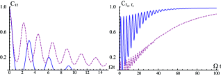
Figure 1: Entanglement between the two atoms (left plots) and between the two reservoirs (right plots) in the good cavity limit for two equal cavities with $\lambda=0.1\Omega$ and for two different detunings: $\delta=\Omega/2$ (solid, blue line) and $\delta=2\Omega$ (dashed, purple line). The initial state is such that $s=0.2$.

As a first example of the time evolution described by the above expressions for the concurrences, we report in Fig. (1) the dynamics of atom-atom entanglement, $C_{1,2}(t)$, and reservoir-reservoir entanglement, $C_{r_{1},r_{2}}(t)$, for two different detunings and for equal cavities, whose parameters are very close to the ideal limit (the photon escape rate is chosen to be ten times smaller the resonant Rabi frequency). Various features should be noted in these plots; let us concentrate on the case with smaller detuning first ($\delta=\Omega/2$, solid lines). Under such conditions, $C_{1,2}$ shows dark periods; that is, time intervals following an ESD, during which the entanglement stays equal to zero before abruptly reviving with a periodicity essentially dictated by the ideal Rabi time, $2\pi/R$. During these dark intervals, $C_{r_{1},r_{2}}$ attains its maxima, and the two concurrences oscillate exactly out of phase. On a time scale essentially set-up by $\lambda$, both of the bipartite entanglement measures are seen to become close to their asymptotic values of $C_{1,2}\rightarrow 0$, and $C_{r_{1},r_{2}}\rightarrow\sqrt{1-s^{2}}$ (the saturation value for the inequality reported above).

One particular aspect that we want to consider here is the effect of the detuning. It was noticed in Ref. [9] that, in the ideal Jaynes-Cummings limit, ESD is quite sensitive to the detunings. The same statement is clearly seen to hold for the reservoir entanglement and for the ESB. Indeed, Fig. (1) shows that by increasing $\delta$, apart from an obvious change in the oscillation period, the time evolution is qualitatively modified as i) the ESD does not occur anymore (and, therefore, no dark intervals are found); ii) it takes a much longer time before the asymptotic values are approached, both for the atom-atom and for the reservoir-reservoir entanglement.

This sensitivity to detunings, however, is seen to be gradually lost as the cavities become more and more leaky. As an example, Fig. (2) reports the same plot as Fig. (1), but for the case $\Omega=\lambda$. It can be seen that, although the time required to almost reach the stationary values is again longer for larger detunings, the huge effect of $\delta$ on the sudden death is not found anymore: the entanglement collapses to zero in both cases and only the ESD-time is affected by $\delta$.

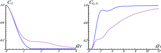
Figure 2: Same as Fig. (1), but with $\lambda=\Omega$. Here too, the solid, blue plots correspond to $\delta=\Omega/2$; while the purple, dashed ones correspond to the $\delta=2\Omega$-case.

By further increasing the ratio $\lambda/\Omega$ (which implies going towards the bad cavity limit), the effect of $\delta$ becomes less and less noticeable.

A similar behavior is found to occur when the two atoms are differently detuned from their cavities. The effect is particularly enhanced when the detunings are opposite in sign (this is reminiscent of what has been found in Ref. [4]). Indeed, by controlling the detuning $\delta=\delta_{1}=-\delta_{2}$, one can qualitatively change the entanglement dynamics and explore regions in which ESD occurs, others in which dark periods or entanglement oscillations are found, eventually reaching parameter regions in which a monotonic long-time decay takes place. As an example, in Fig. (3), we report four different behaviors of the atom-atom entanglement, obtained, for an intermediate coupling regime with the cavities, by just changing the detunings.

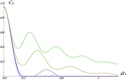
Figure 3: Atom-atom entanglement, $C_{1,2}(t)$, evaluated in the case of equal cavities with $\Omega=2.5\lambda$ and with an atomic initial condition set by $s=0.3$. The four plots (starting from below) refer to symmetrically detuned atoms with $\delta_{1}/\Omega\equiv-\delta_{2}/\Omega=0,1,2,3$ (solid, dashed, dotted and dot-dashed lines, respectively).

4 Entanglement Generation

In this section we describe some schemes for generating entanglement among one of the atoms and the two cavities, between the two cavity fields, and between one atom and a distant cavity. These schemes are based on the assumption that one can control the couplings between each atom and its surrounding cavity field as well as the atom-cavity interaction time. Both these requirements are experimentally feasible, e.g., in ion cavity QED systems, since the effective atom-cavity coupling is achieved via laser driven two-photon processes. The effective atom-cavity coupling in this case is given by $g_{\rm eff}=g\Omega/\Delta$, with $g$ the cavity coupling constant, $\Omega$ the Rabi frequency of the laser driving the Raman transition, and $\Delta$ the laser and cavity detuning from an excited third level [16]. In this case, $g_{\rm eff}$ can be controlled by changing the laser intensity and/or detuning while the interaction time is determined by the length of the laser pulse.

4.1 Generation of W-states

Inserting Eq. (4) into Eq. (3), we can explicitly write the total state in terms of its five components, as follows

$$\left|\psi,t\right\rangle = \sqrt{\frac{1-s}{2}}\left|g_{1}g_{2}\right\rangle\bigotimes_{k_{1}k_{2}}\left|0_{k_{1}}0_{k_{2}}\right\rangle$$ (14)

$$+ e^{i\varphi}\sqrt{\frac{1+s}{2}}\Big{[}{\cal E}_{1}(t){\cal E}_{2}(t)\left|e_{1}e_{2}\right\rangle\otimes\left|0_{k_{1}}0_{k_{2}}\right\rangle$$

$$+ {\cal E}_{1}(t){\cal F}_{2}(t)\left|e_{1}g_{2}\right\rangle\otimes\left|0_{k_{1}},\mbox{\mbox{photon}}_{2}\right\rangle$$

$$+ {\cal F}_{1}(t){\cal E}_{2}(t)\left|g_{1}e_{2}\right\rangle\otimes\left|\mbox{\mbox{photon}}_{1},0_{k_{2}}\right\rangle$$

$$+ {\cal F}_{1}(t){\cal F}_{2}(t)\left|g_{1}g_{2}\right\rangle\otimes\left|\mbox{\mbox{photon}}_{1},\mbox{\mbox{photon}}_{2}\right\rangle\Big{]}.$$

We note that, at a time $\bar{t}$ such that ${\cal F}_{1}(\bar{t})\simeq 1$ and ${\cal E}_{1}(\bar{t})\simeq 0$, the state of the system approximates

$$\left|\psi^{\prime}(\bar{t})\right\rangle \simeq \Big{\{}\sqrt{\frac{1-s}{2}}\left|g_{2}\right\rangle\bigotimes_{k_{1}k_{2}}\left|0_{k_{1}}0_{k_{2}}\right\rangle$$

$$+ e^{i\varphi}\sqrt{\frac{1+s}{2}}\Big{[}{\cal E}_{2}(\bar{t})\left|e_{2}\right\rangle\otimes\left|\mbox{\mbox{photon}}_{1},0_{k_{2}}\right\rangle$$

$$+ (\bar{t}){\cal F}_{2}(\bar{t})\left|g_{2}\right\rangle\otimes\left|\mbox{\mbox{photon}}_{1},\mbox{\mbox{photon}}_{2}\right\rangle\Big{]}\Big{\}}\left|g_{1}\right\rangle,$$

From this equation one sees immediately that for $s=1/3$ and ${\cal E}_{2}(\bar{t})=\frac{1}{\sqrt{2}}$ one obtains the W-state

$$\left|\psi_{W}\right\rangle=\frac{1}{\sqrt{3}}\left(\left|010\right\rangle+\left|100\right\rangle+\left|001\right\rangle\right),$$ (16)

with

$$\left|010\right\rangle = \left|g_{2}\right\rangle\bigotimes_{k_{1}k_{2}}\left|0_{k_{1}}0_{k_{2}}\right\rangle,$$ (17)

$$\left|100\right\rangle = \left|e_{2}\right\rangle\bigotimes_{k_{2}}\left|\mbox{\mbox{photon}}_{1},0_{k_{2}}\right\rangle,$$ (18)

$$\left|001\right\rangle = \left|g_{2}\right\rangle\left|\mbox{\mbox{photon}}_{1},\mbox{\mbox{photon}}_{2}\right\rangle.$$ (19)

Assuming an intermediate coupling regime for the first cavity, e.g., $\Omega_{1}=\lambda_{1}$, and taking for simplicity $\delta_{1}=0$, we see from Eqs. (5)- (6) that ${\cal F}_{1}(\bar{t})\approx 0.99$ at $\lambda_{1}\bar{t}=3$. The condition ${\cal E}_{2}(\bar{t})=\frac{1}{\sqrt{2}}$ is then obtained for $\Omega_{2}\simeq 0.4\lambda_{2}$, with $\lambda_{1}=\lambda_{2}$ and $\delta_{2}=0$.

4.2 Generation of Bell states

W-states are characterized by the property that bipartite entanglement can be obtained after the measurement of any of the three parties. In our case, measuring the atomic state of the second atom in $\left|g_{2}\right\rangle$ generates a maximally entangled state of the cavity fields of the type

$$\left|\psi_{r_{1}r_{2}}\right\rangle=\frac{1}{\sqrt{2}}\left(\bigotimes_{k_{1}k_{2}}\left|0_{k_{1}}0_{k_{2}}\right\rangle+\left|\mbox{\mbox{photon}}_{1},\mbox{\mbox{photon}}_{2}\right\rangle\right).$$ (20)

The generation of a W-state followed by a measurement of the second atom in its ground state is similar to entanglement swapping, since it amounts at transferring entanglement from the atoms pairs to two fields inside two distinct non-interacting cavities.

A Bell state of the atom-cavity system of the second atom can be generated by measuring the presence of a photon in the other cavity. In this case the state generated is

$$\left|\psi_{a_{2}r_{2}}\right\rangle=\frac{1}{\sqrt{2}}\left(\bigotimes_{k_{2}}\left|e_{2}0_{k_{2}}\right\rangle+\left|g_{2},\mbox{\mbox{photon}}_{2}\right\rangle\right).$$ (21)

Most intriguingly, finally, a measurement of the cavity 2 in the vacuum creates a maximally entangles state of the atom 2 with the cavity 1,

$$\left|\psi_{a_{2}r_{1}}\right\rangle=\frac{1}{\sqrt{2}}\left(\bigotimes_{k_{1}}\left|g_{2}0_{k_{1}}\right\rangle+\left|e_{2},\mbox{\mbox{photon}}_{1}\right\rangle\right).$$ (22)

Finally we note that a similar W-state can be obtained by requiring that ${\cal F}_{2}(t)\simeq 1$ and ${\cal E}_{2}(t)\simeq 0$. The results are exactly the same as the ones discussed above provided that one exchanges atom 1 with atom 2.

5 Summary and conclusions

We have discussed various features related to the transfer of quantum correlation due to the interaction of a pair of atoms (qubit) with two independent bosonic reservoirs, having non-markovian features. In particular, we have taken a Lorentzian spectral density for each reservoir, in order to mimic the nearly resonant coupling of initially entangled atoms to leaky cavities [19]. In such a case, the Hamiltonian model is amenable to an exact solution, so that the time evolution of various bipartite entanglement measures can be easily evaluated. In particular, we focussed on the atom-atom and reservoir-reservoir entanglement to show that: 1) the initial atomic entanglement is found to be transferred to the reservoirs; 2) the dynamics of the entanglement is strongly sensitive to the detuning of the atoms from their cavities, so that the detuning can be used as a knob to qualitatively change the character of the time evolution of the quantum correlations. These conclusions hold true in any atom-cavity coupling regime, ranging from ideal cavity (strong coupling regime) with a monochromatic spectral density, to a markovian environment with an almost structure-less environmental spectral density (bad cavity or weak coupling limit). Although the sensitivity to the detuning diminishes by going towards the markovian limit, we have found that an enhanced sensitivity can be obtained by independently controlling the two atomic detunings; and, in particular, that the entanglement time-evolution can be substantially altered if the two atoms are symmetrically out of resonance with respect to their cavities.

We have also discussed a protocol to deterministically generate a W-state with one atom and two cavity fields, which can subsequently be used as a starting point for probabilistic schemes aimed at generating maximally entangled states of one atom and one, distant cavity field, and of the two cavity fields. It is worth mentioning that these schemes are designed by taking into account the cavity losses and that they work despite their presence.

References

- [1] T. Yu and J. H. Eberly, Phys. Rev. Lett. 93 (2004) 140404; T. Yu and J. H. Eberly, Phys. Rev. Lett. 97 (2006) 140403; T. Yu and J. H. Eberly, Science 323 (2009) 598.
- [2] M. P. Almeida et al., Science 316 (2007) 579.
- [3] J. Laurat et al., Phys. Rev. Lett. 99 (2007) 180504.
- [4] S. Maniscalco et al., Phys. Rev. Lett. 100 (2008) 090503; F. Francica et al., Phys. Rev. A 79 (2009) 032310; F. Francica, F. Plastina and S. Maniscalco, Phys. Rev. A 82 (2010) 052118.
- [5] B. Bellomo, R. Lo Franco, and G. Compagno, Phys. Rev. Lett. 99 (2007) 160502; B. Bellomo, R. Lo Franco, and G. Compagno, Phys. Rev. A 77 (2008) 032342.
- [6] S. Cialdi, D. Brivio, E. Tesio, M. G. A. Paris, Phys. Rev. A 83 (2011) 042308.
- [7] A. Al-Qasimi and D. F. V. James, Phys. Rev. A 77 (2008) 012117.
- [8] J. Jing, Z.-G. Lü and Z. Ficek, Phys. Rev. A 79 (2009) 044305.
- [9] S. Chan, M. D. Reid and Z. Ficek, J. Phys. B: At. Mol. Opt. Phys. 42 (2009) 065507.
- [10] F. Altintas and R. Eryigit, J. Phys. B: At. Mol. Opt. Phys. 44 (2011) 125501.
- [11] C. E. López et al., Phys. Rev. Lett. 101 (2008) 080503.
- [12] M. Yönaç, T. Yu and J. H. Eberly, J. Phys. B: At. Mol. Opt. Phys. 39 (2006) S621; M. Yönaç M., T. Yu and J. H. Eberly, J. Phys. B: At. Mol. Opt. Phys. 40 (2007) S45.
- [13] Q.-H. Chen, Y. Yang, T. Liu, K.-L. Wang, Phys. Rev. A 82 (2010) 052306.
- [14] I. Sainz and G. Björk, Phys. Rev. A 76 (2007) 042313; S. Chan, M. D. Reid and Z. Ficek, J. Phys. B: At. Mol. Opt. Phys. 43 (2010) 215505; C. E. López, G. Romero, and J. C. Retamal, Phys. Rev. A, 81 (2010) 062114; Z.-X. Man, Y.-J. Xia, N. B. An, J. Phys. B: At. Mol. Opt. Phys. 44 (2011) 095504.
- [15] Z. Y. Xu and M. Feng, Phys. Lett A 373 (2009) 1906; Y. J. Zhang, Z. X. Man and Y. J. Xia, Eur. Phys. J. D 55 (2009) 173.
- [16] K. Härkönen, F. Plastina, and S. Maniscalco, Phys. Rev. A 80 (2009) 033841.
- [17] W. K. Wootters, Phys. Rev. Lett. 80 (1998) 2245.
- [18] Q.-J. Tong, J.-H. An, H.-G. Luo, C. H. Oh, arXiv:1005.1001 (2011).
- [19] L. Mazzola, S. Maniscalco, J. Piilo, K.-A. Suominen, and B. M. Garraway, Phys. Rev. A 80 (2009) 012104.