Approximating Tverberg Points in Linear Time for Any Fixed Dimension

Abstract

Let $P\subseteq\mathbb{R}^{d}$ be a $d$-dimensional $n$-point set. A Tverberg partition is a partition of $P$ into $r$ sets $P_{1},\dots,P_{r}$ such that the convex hulls $\operatorname{conv}(P_{1}),\dots,\operatorname{conv}(P_{r})$ have non-empty intersection. A point in $\bigcap_{i=1}^{r}\operatorname{conv}(P_{i})$ is called a Tverberg point of depth $r$ for $P$. A classic result by Tverberg shows that there always exists a Tverberg partition of size $\lceil n/(d+1)\rceil$, but it is not known how to find such a partition in polynomial time. Therefore, approximate solutions are of interest.

We describe a deterministic algorithm that finds a Tverberg partition of size $\lceil n/4(d+1)^{3}\rceil$ in time $d^{O(\log d)}n$. This means that for every fixed dimension we can compute an approximate Tverberg point (and hence also an approximate centerpoint) in linear time. Our algorithm is obtained by combining a novel lifting approach with a recent result by Miller and Sheehy [13].

Keywords. discrete geometry, Tverberg theorem, centerpoint, approximation, high dimension

1 Introduction

In many applications (such as statistical analysis or finding sparse geometric separators in meshes) we would like to have a way to generalize the one-dimensional notion of a median to higher dimensions. A natural way to do this uses the notion of halfspace depth (or Tukey depth).

Definition 1

Let $P$ be a finite set of points in $\mathbb{R}^{d}$, and let $c\in\mathbb{R}^{d}$ be a point (not necessarily in $P$). The halfspace depth of $c$ with respect to $P$ is

$$\min_{\textnormal{halfspace }h,\,c\in h}|h\cap P|.$$

The halfspace depth of $P$ is the maximum halfspace depth that any point $c\in\mathbb{R}^{d}$ can achieve.

A classic result in discrete geometry, the Centerpoint Theorem, claims that for every $d$-dimensional point set $P$ with $n$ points there exists a centerpoint, i.e., a point $c\in\mathbb{R}^{d}$ with halfspace depth at least $n/(d+1)$ [6, 15]. There are point sets where this bound cannot be improved.

However, if we actually want to compute a centerpoint for a given point set efficiently, the situation becomes more involved. For $d=2$, a centerpoint can be found deterministically in linear time [9]. For general $d$, we can compute a centerpoint in $O(n^{d})$ time using linear programming, since Helly’s theorem implies that the set of all centerpoints can be described as the intersection of $O(n^{d})$ halfspaces [7]. Chan [2] shows how to improve this running time to $O(n^{d-1})$ with the help of randomization. He actually solves the apparently harder problem of finding a point with maximum halfspace depth. If the dimension is not fixed, a result by Teng shows that it is coNP-hard to check whether a given point is a centerpoint [17].

However, as $d$ grows, a running time of $n^{\Omega(d)}$ is not feasible. Hence, it makes sense to look for faster approximate solutions. A classic approach uses $\varepsilon$-approximations [3]: in order to obtain a point of halfspace depth $n(1/(d+1)-\varepsilon)$, take a random sample $A\subseteq P$ of size $O((d/\varepsilon^{2})\log(d/\varepsilon))$ and compute a centerpoint for $A$ via linear-programming. This gives the desired approximation with constant probability, and the running time after the sampling step is constant for fixed $d$. What more could we possibly wish for? For one, the algorithm is Monte-Carlo: with a certain probability, the reported point fails to be a centerpoint, and we know of no fast algorithm to check its validity. This problem can be solved by constructing the $\varepsilon$-approximation deterministically [3], at the expense of a more complicated algorithm. Nonetheless, in either case the resulting running time grows exponentially with $d$, an undesirable feature for large dimensions.

This situation motivated Clarkson et al. [4] to look for more efficient randomized algorithms for approximate centerpoints. They give a simple probabilistic algorithm that computes a point of halfspace depth $\Omega(n/(d+1)^{2})$ in time $O(d^{2}(d\log n+\log(1/\delta))^{\log(d+2)})$, where $\delta$ is the error probability. They also describe a more sophisticated algorithm that finds such a point in time polynomial in $n$, $d$, and $\log(1/\delta)$. Both algorithms are based on a repeated algorithmic application of Radon’s theorem (see below). Unfortunately, there remains a probability of $\delta$ that the result is not correct, and we do not know how to detect failure efficiently.

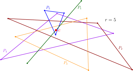
Figure 1: The point $c$ has Tverberg depth $r=5$.

Thus, more than ten years later, Miller and Sheehy [13] launched a new attack on the problem. Their goal was to develop a deterministic algorithm for approximating centerpoints whose running time is subexponential in the dimension. For this, they use a different proof of the centerpoint theorem that is based on a result by Tverberg: any $d$-dimensional $n$-point set can be partitioned into $r=\lceil n/(d+1)\rceil$ sets $P_{1},\dots,P_{r}$ such that the convex hulls $\operatorname{conv}(P_{1}),\dots,\operatorname{conv}(P_{r})$ have nonempty intersection. Such a partition is called a Tverberg partition of $P$. By convexity, any point in $\bigcap_{i=1}^{r}\operatorname{conv}(P_{i})$ must be a centerpoint.

More generally, we say that a point $c\in\mathbb{R}^{d}$ has Tverberg depth $r^{\prime}$ with respect to $P$ if there is a partition of $P$ into $r^{\prime}$ sets such that $c$ lies in the convex hull of each set. We also call $c$ an approximate Tverberg point (of depth $r^{\prime}$); see Figure 1.

Miller and Sheehy describe how to find $\lceil n/2(d+1)^{2}\rceil$ disjoint subsets of $P$ and a point $c\in\mathbb{R}^{d}$ such that each subset contains $d+1$ points and has $c$ in its convex hull. Hence, $c$ constitutes an approximate Tverberg point for $P$ (and thus also an approximate centerpoint), and the subsets provide a certificate for this fact. The algorithm is deterministic and runs in time $n^{O(\log d)}$. At the same time, it is the first algorithm that also finds an approximate Tverberg partition of $P$. The running time is subexponential in $d$, but it is still the case that $n$ is raised to a power that depends on $d$, so the parameters $n$ and $d$ are not separated in the running time.

In this paper, we show that the running time for finding approximate Tverberg partitions (and hence approximate centerpoints) can be improved. In particular, we show how to find a Tverberg partition with $\lceil n/4(d+1)^{3}\rceil$ sets in deterministic time $d^{O(\log d)}n$. This is linear in $n$ for any fixed dimension, and the dependence on $d$ is only quasipolynomial.

1.1 Some Discrete Geometry

We begin by recalling some basic facts and definitions from discrete geometry [11]. A classic fact about convexity is Radon’s theorem.

Theorem 1.1 (Radon’s theorem)

For any $P\subseteq\mathbb{R}^{d}$ with $d+2$ points there exists a partition $(P_{1},P_{2})$ of $P$ such that $\operatorname{conv}(P_{1})\cap\operatorname{conv}(P_{2})\neq\emptyset$.

As mentioned above, Tverberg [18] generalized this theorem for larger point sets.

Theorem 1.2 (Tverberg’s theorem)

Any set $P\subseteq\mathbb{R}^{d}$ with $n=(r-1)(d+1)+1$ points can be partitioned into $r$ sets $P_{1},\dots,P_{r}$ such that $\bigcap_{i=1}^{r}\operatorname{conv}(P_{i})\neq\emptyset$.

Let $P$ be a set of $n$ points in $\mathbb{R}^{d}$. We say that $x\in\mathbb{R}^{d}$ has Tverberg depth $r$ (with respect to $P$) if there is a partition of $P$ into sets $P_{1},\dots,P_{r}$ such that $x\in\bigcap_{i=1}^{r}\operatorname{conv}(P_{i})$. Tverberg’s theorem thus states that, for any set $P$ in $\mathbb{R}^{d}$, there is a point of Tverberg depth at least $\lfloor(n-1)/(d+1)+1\rfloor=\lceil n/(d+1)\rceil$. Note that every point with Tverberg depth $r$ also has halfspace depth $r$. Thus, from now on we will use the term depth as a shorthand for Tverberg depth. As remarked above, Tverberg’s theorem immediately implies the famous Centerpoint Theorem (see [11]):

Theorem 1.3 (Centerpoint Theorem)

For any set $P$ of $n$ points in $\mathbb{R}^{d}$ there is a point $c$ such that all halfspaces containing $c$ contain at least $\lceil n/(d+1)\rceil$ points from $P$.

Finally, another classic theorem will be useful for us.

Theorem 1.4 (Carathéodory’s theorem)

Suppose that $P$ is a set of $n$ points in $\mathbb{R}^{d}$ and $x\in\operatorname{conv}(P)$. Then there is a set of $d+1$ points $P^{\prime}\subseteq P$ such that $x\in\operatorname{conv}(P^{\prime})$.

This means that, in order to describe a Tverberg partition of depth $r$, we need only $r(d+1)$ points from $P$. This observation is also used by Miller and Sheehy [13]. They further note that it takes $O(d^{3})$ time to replace $d+2$ points by $d+1$ points by using Gaussian elimination. We denote the process of replacing larger sets by sets of size $d+1$ as pruning, see Lemma 2.2.

1.2 Our Contribution

We now describe our results in more detail. In Section 2, we present a simple lifting argument which leads to an easy Tverberg approximation algorithm.

Theorem 1.5

Let $P$ be a set of $n$ points in $\mathbb{R}^{d}$ in general position. One can compute a Tverberg point of depth $\lceil n/2^{d}\rceil$ for $P$ and the corresponding partition in time $d^{O(1)}n$.

While this does not yet give a good approximation ratio (though constant for any fixed $d$), it is a natural approach to the problem: it computes a higher dimensional Tverberg point via successive median partitions—just as a Tverberg point is a higher dimensional generalization of the $1$-dimensional median.

By collecting several low-depth points and afterwards applying the brute-force algorithm on small point sets, we get an even higher depth in linear time for any fixed dimension:

Theorem 1.6

Let $P$ be a set of $n$ points in $\mathbb{R}^{d}$. Then one can find a Tverberg point of depth $\lceil n/2(d+1)^{2}\rceil$ and a corresponding partition in time $f(2^{d+1})+d^{O(1)}n$, where $f(m)$ is the time to compute a Tverberg point of depth $\lceil m/(d+1)\rceil$ for $m$ points by brute force.

Finally, by combining our approach with that of Miller and Sheehy, we can improve the running time to be quasipolynomial in $d$:

Theorem 1.7

Let $P$ be a set of $n$ points in $\mathbb{R}^{d}$. Then one can compute a Tverberg point of depth $\lceil n/4(d+1)^{3}\rceil$ and a corresponding pruned partition in time $d^{O(\log d)}n$.

In Section 4, we compare these results to the Miller-Sheehy algorithm and its extensions.

2 A Simple Fixed-Parameter Algorithm

We now present a simple algorithm that runs in linear time for any fixed dimension and computes a point of depth $\lceil n/2^{d}\rceil$. For this, we show how to compute a Tverberg point by recursion on the dimension. As a byproduct, we obtain a quick proof of a weaker version of Tverberg’s theorem. First, however, we give a few more details about the basic operations performed by our algorithm.

2.1 Basic Operations

Our algorithm builds a Tverberg partition for a $d$-dimensional point set $P$ by recursion on the dimension. In each step, we store a Tverberg partition for some point set, together with an approximate Tverberg point $c$. We have for each set $P_{i}$ in the partition a convex combination that witnesses $c\in\operatorname{conv}(P_{i})$. All the points that arise during our algorithms are obtained by repeatedly taking convex combinations of the input points, so the following simple observation lets us maintain this invariant.

Observation 2.1

If $x_{i}=\sum_{p\in P_{i}}\alpha_{p}p$ and $y=\sum_{i}\beta_{i}x_{i}$ are convex combinations, then

$$y=\sum_{i}\sum_{p\in P_{i}}\beta_{i}\alpha_{p}p$$

is a convex combination of the set $\bigcup P_{i}$ for $y$. ∎

By Carathéodory’s theorem (Theorem 1.4), a Tverberg partition of depth $r$ can be described by $r(d+1)$ points from $P$. In order to achieve running time $O(n)$, we need the following observation, also used by Miller and Sheehy [13].

Lemma 2.2

Let $Q\subseteq\mathbb{R}^{d}$ be a set of $m\geq d+2$ points with $c\in\operatorname{conv}(Q)$, and suppose we have a convex combination of $Q$ for $c$. Then we can find a subset $Q^{\prime}\subset Q$ with $d+1$ points such that $c\in\operatorname{conv}(Q^{\prime})$, together with a corresponding convex combination, in time $O(d^{3}m)$.

Proof

Miller and Sheehy observe that replacing $d+2$ points by $d+1$ points takes $O(d^{3})$ time by finding an affine dependency through Gaussian elimination, see Grötschel, Lovász, and Schrijver [8, Chapter 1]. The choice of affine dependencies does not matter. Thus, in order to eliminate a point from $Q$, we can take any subset of size $d+2$, resolve one of the affine dependencies, and update the convex combination accordingly. Repeating this process, we can replace $m$ points by $d+1$ points in time $(m-(d+1))O(d^{3})=O(d^{3}m)$. ∎

The process in Lemma 2.2 is called pruning, and we call a partition of a $d$-dimensional point set in which all sets have size at most $d+1$ a pruned partition. This will enable us to bound the cost of many operations in terms of the dimension $d$, instead of the number of points $n$.

2.2 The Lifting Argument and a Simple Algorithm

Let $P$ be a $d$-dimensional point set. As a Tverberg point is a higher dimensional version of the median, a natural way to compute a Tverberg point for $P$ is to first project $P$ to some lower-dimensional space, then to recursively compute a good Tverberg point for this projection, and to use this point to find a solution in the higher-dimensional space. Surprisingly, we are not aware of any such argument having appeared in the literature so far.

In what follows, we will describe how to lift a lower-dimensional Tverberg point into some higher dimension. Unfortunately, this process will come at the cost of a decreased depth for the lifted Tverberg point. For clarity of presentation, we first explain the lifting lemma in its simplest form. In Section 3.1, we then state the lemma in its full generality.

(a) project

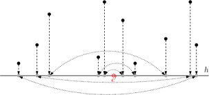
(b) find partition

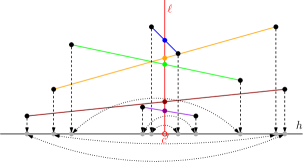
(c) intersect hulls of the sets with $h^{\perp}$

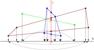
(d) find median of intersections and combine

Figure 2: Illustrating the lifting lemma in the plane: we project the point set $P$ to the line $h$ and find a Tverberg partition and a Tverberg point $c^{\prime}$ for the projection. Then, we construct the line $\ell$ through $c^{\prime}$ that is perpendicular to $h$, and we take the intersection with the lifted convex hulls of the Tverberg partition. We then find the median $c$ and the corresponding partition for the intersections along $\ell$. Finally, we group the points according to this partition.

Lemma 2.3

Let $P$ be a set of $n$ points in $\mathbb{R}^{d}$, and let $h$ be a hyperplane in $\mathbb{R}^{d}$. Let $c^{\prime}\in h$ be a Tverberg point of depth $r$ for the projection of $P$ onto $h$, with pruned partition $P_{1},\dots,P_{r}$. Then we can find a Tverberg point $c\in\mathbb{R}^{d}$ of depth $\lceil r/2\rceil$ for $P$ and a corresponding Tverberg partition in time $O(dn)$.

Proof

For every point $p\in P$, let $\operatorname{pr}(p)$ denote the projection of $p$ onto $h$, and for every $Q\subseteq P$, let $\operatorname{pr}(Q)$ be the projections of all the points in $Q$. Let $P_{1},\dots,P_{r}\subseteq P$ such that $\operatorname{pr}(P_{1}),\dots,\operatorname{pr}(P_{r})$ is a pruned partition for $\operatorname{pr}(P)$ with Tverberg point $c^{\prime}$. Let $\ell$ be the line through $c^{\prime}$ orthogonal to $h$.

Since our assumption implies $c^{\prime}\in\operatorname{conv}(\operatorname{pr}(P_{i}))$ for $i=1,\dots,r$, it follows that $\ell$ intersects each $\operatorname{conv}(P_{i})$ at some point $x_{i}\in\mathbb{R}^{d}$. More precisely, as we have a convex combination $c^{\prime}=\sum_{p\in P_{i}}\alpha_{p}\operatorname{pr}(p)$ for each $P_{i}$, we simply get $x_{i}=\sum_{p\in P_{i}}\alpha_{p}p$.

Assuming an appropriate numbering, let $\widehat{Q}_{i}=\left\{x_{2i-1},x_{2i}\right\}$, $i=1,\dots,\lceil r/2\rceil$, be a Tverberg partition of $x_{1},\dots,x_{r}$. (If $r$ is odd, the set $\widehat{Q}_{\lceil r/2\rceil}$ contains only one point, the median.) Since the points $x_{i}$ lie on the line $\ell$, such a Tverberg partition exists and can be computed in time $O(r)$ by finding the median $c$, i.e., the element of rank $\lceil r/2\rceil$, according to the order along $\ell$ (see Cormen et al. [5, Chapter 9]). We claim that $c$ is a Tverberg point for $P$ of depth $\lceil r/2\rceil$. Indeed, we have

$$c\in\operatorname{conv}(\widehat{Q}_{i})=\operatorname{conv}(\left\{x_{2i-1},x_{2i}\right\})\subseteq\operatorname{conv}(P_{2i-1}\cup P_{2i}),$$

for $1\leq i\leq\lceil r/2\rceil$. Thus, if we set $Q_{i}:=P_{2i-1}\cup P_{2i}$, then $Q_{1},\dots,Q_{\lceil r/2\rceil}$ is a Tverberg partition for the point $c$. The total time to compute $c$ and the $Q_{i}$ is $O(n)$, as claimed. See Figure 2 for a two-dimensional illustration of the lifting argument. ∎

Theorem 1.5 is now a direct consequence of Lemma 2.3.

Theorem 2.4 (Thm 1.5, restated)

Let $P$ be a set of $n$ points in $\mathbb{R}^{d}$ in general position. One can compute a Tverberg point of depth $\lceil n/2^{d}\rceil$ for $P$ and the corresponding partition in time $d^{O(1)}n$.

Proof

If $d=1$, we obtain a Tverberg point and a corresponding partition by finding the median $c$ of $P$ [5] and pairing each point to the left of $c$ with exactly one point to the right of $c$.

If $d>1$, we project $P$ onto the hyperplane $x_{d}=0$. This gives an $n$-point set $P^{\prime}\subseteq\mathbb{R}^{d-1}$. We recursively find a point of depth $\lceil n/{2^{d-1}}\rceil$ and a corresponding pruned partition for $P^{\prime}$. We then apply Lemma 2.3 to get a point $c\in\mathbb{R}^{d}$ of depth $r=\left\lceil\lceil n/{2^{d-1}}\rceil/2\right\rceil\geq\lceil n/2^{d}\rceil$ for $P$, together with a partition. Each set has at most $2d$ points, so by applying Lemma 2.2 to each set, it takes $O(d^{4}r)$ time to prune all sets.

This yields a total running time of $T_{d}(n)\leq T_{d-1}(n)+d^{O(1)}n$, which implies the result. ∎

In particular, Theorem 1.5 gives a weak version of Tverberg’s theorem with a simple proof.

Corollary 2.5 (Weak Tverberg theorem)

Let $P$ be a set of $n$ points in $\mathbb{R}^{d}$. Then $P$ can be partitioned into $\lceil n/2^{d}\rceil$ sets $P_{1},\dots,P_{\lceil n/2^{d}\rceil}$ such that

$$\bigcap_{i=1}^{\lceil n/2^{d}\rceil}\operatorname{conv}(P_{i})\neq\emptyset.$$

∎

2.3 An Improved Approximation Factor

In order to improve the approximation factor, we will now use an easy bootstrapping approach. A Tverberg partition of depth $r$ in $\mathbb{R}^{d}$ needs only $(d+1)r$ points. This means that after finding a point of depth $n/2^{d}$, we still have $n\left(1-(d+1)/2^{d}\right)$ unused points at our disposal. The next lemma shows how to leverage these points to achieve an even higher Tverberg depth.

Lemma 2.6

Let $\rho\geq 2$ and $q(m,d)$ be a function such that for any $m$-point set $Q\subseteq\mathbb{R}^{d}$ we can compute a point of depth $\lceil m/\rho\rceil$ and a corresponding pruned partition in time $q(m,d)$.

Let $P\subseteq\mathbb{R}^{d}$ with $|P|=n$, and let $\beta\in[2,n/\rho]$ be a constant. Define the target depth $\delta$ as $\delta:=\lceil n/\beta\rho\rceil$. Then we can find $\alpha:=\lceil\frac{n(1-1/\beta)}{\delta(d+1)}\rceil$ disjoint subsets $Q_{1},\dots,Q_{\alpha}$ of $P$ such that for each $Q_{i}$ we have a Tverberg point $c_{i}$ of depth $\delta$ and a pruned partition $\mathcal{Q}_{i}$. This takes total time

$$O\Biggl{(}\frac{(\beta-1)\rho\,q(n,d)}{d+1}\Biggr{)}.$$

Proof

Let $P_{1}:=P$. We take an arbitrary subset $P_{1}^{\prime}\subseteq P_{1}$ with $\lceil n/\beta\rceil$ points and find a Tverberg point $c_{1}$ of depth $\delta$ and a corresponding pruned partition $\mathcal{Q}_{1}$ for $P^{\prime}_{1}$. This takes time $q(n,d)$, and the set $Q_{1}:=\bigcup_{Z\in\mathcal{P}_{1}}Z$ contains at most $\delta(d+1)$ points. Set $P_{2}:=P_{1}\setminus Q_{1}$ and repeat. The resulting sets $Q_{i}$ are pairwise disjoint, and we can repeat this process until

$$n-i\delta(d+1)<\frac{n}{\beta}.$$

This gives

$$\alpha\geq i>\left\lceil\frac{n(1-1/\beta)}{\delta(d+1)}\right\rceil.$$

Thus, we obtain $\alpha$ points $c_{1},\dots,c_{\alpha}$ with corresponding Tverberg partitions $\mathcal{Q}_{1},\dots,\mathcal{Q}_{\alpha}$, each of depth at least $\lceil n/\beta\rho\rceil$, as desired. ∎

For example, by Theorem 1.5 we can find a point of depth $\lceil n/2^{d}\rceil$ and a corresponding pruned partition in time $d^{O(1)}n$. Thus, by applying Lemma 2.6 with $c=2$, $\rho=2^{d}$, we can also find $\lceil n/(2\lceil n/2^{d+1}\rceil(d+1))\rceil\approx 2^{d}/(d+1)$ points of depth $\lceil n/2^{d+1}\rceil$ in linear time.

In order to make use of Lemma 2.6, we will also need a lemma that describes how we can combine these points in order to increase the total depth. This generalizes a similar lemma by Miller and Sheehy [13, Lemma 4.1].

Lemma 2.7

Let $P$ be a set of $n$ points in $\mathbb{R}^{d}$, and let $P=\biguplus_{i=1}^{\alpha}P_{i}$ be a partition of $P$. Furthermore, suppose that for each $P_{i}$ we have a Tverberg point $c_{i}\in\mathbb{R}^{d}$ of depth $r$, together with a corresponding pruned partition $\mathcal{P}_{i}$. Let $C:=\{c_{i}\mid 1\leq i\leq\alpha\}$ and $c$ be a point of depth $r^{\prime}$ for $C$, with corresponding pruned partition $\mathcal{C}$. Then $c$ is a point of depth $rr^{\prime}$ for $P$. Furthermore, we can find a corresponding pruned partition in time $d^{O(1)}n$.

Proof

For $i=1,\dots,\alpha$, write $\mathcal{P}_{i}=\{Q_{i1},\dots,Q_{ir}\}$, and write $\mathcal{C}=\{D_{1},\dots,D_{r^{\prime}}\}$. For $a=1,\dots,r^{\prime}$, $b=1,\dots,r$, we define sets $Z_{ab}$ as

$$Z_{ab}:=\bigcup_{c_{i}\in D_{a}}Q_{ib}.$$

We claim that the set $\mathcal{Z}:=\{Z_{ab}\mid a=1,\dots,r^{\prime};b=1,\dots,r\}$ is a Tverberg partition of depth $rr^{\prime}$ for $P$ with Tverberg point $c$. By definition, $\mathcal{Z}$ is a partition with the appropriate number of elements. It only remains to check that $c\in\operatorname{conv}(Z_{ab})$ for each $Z_{ab}$. Indeed, we have

$$c\in\operatorname{conv}(D_{a})=\operatorname{conv}\left(\bigcup_{c_{i}\in D_{a}}\left\{c_{i}\right\}\right)\subseteq\operatorname{conv}\Bigl{(}\bigcup_{c_{i}\in D_{a}}\operatorname{conv}\left(Q_{ib}\right)\Bigr{)}=\operatorname{conv}\Bigl{(}\bigcup_{c_{i}\in D_{a}}Q_{ib}\Bigr{)}=\operatorname{conv}(Z_{ab}),$$

for $a=1\dots r^{\prime},b=1\dots r$.

As the partitions $\mathcal{P}_{i}$ and $\mathcal{C}$ were pruned, each $Z_{ab}$ consists of at most $(d+1)^{2}$ points. Thus, by Lemma 2.2, each $Z_{ab}$ can be pruned in time $O(d^{5})$. Since $|\mathcal{Z}|\leq n$, the lemma follows. ∎

Combining Lemmas 2.6 and 2.7, we can now prove Theorem 1.6.

Theorem 2.1 (Thm 1.6, restated)

Let $P$ be a set of $n$ points in $\mathbb{R}^{d}$. Then one can find a Tverberg point of depth $\lceil n/2(d+1)^{2}\rceil$ and a corresponding partition in time $f(2^{d+1})+d^{O(1)}n$, where $f(m)$ is the time to compute a Tverberg point of depth $\lceil m/(d+1)\rceil$ for $m$ points by brute force, together with an associated Tverberg partition.

Proof

If $n\leq 2^{d+1}$, we solve the problem by brute-force in $f(2^{d+1})$ time. Otherwise, we apply Lemma 2.6 with $c=2$ and $\rho=2^{d}$ to obtain a set $C$ of

$$|C|=\left\lceil\frac{n}{2\lceil n/2^{d+1}\rceil(d+1)}\right\rceil$$

points of depth $\lceil n/2^{d+1}\rceil$ for $P$ with corresponding pruned partitions in time $d^{O(1)}n$. We then use the brute-force algorithm to get a Tverberg point for $C$ with depth $\lceil|C|/(d+1)\rceil$ and a corresponding partition, in time $f(|C|)$. Finally, we apply Lemma 2.7 to obtain a Tverberg point and corresponding partition in time $d^{O(1)}n$. Using that $\lceil a\lceil b\rceil\rceil\geq\lceil ab\rceil$ and $\lceil a\rceil\lceil b\rceil\geq\lceil a\lceil b\rceil\rceil$ for $a,b\geq 0$, we get that the resulting depth is

$$\left\lceil\frac{n}{2^{d+1}}\right\rceil\cdot\left\lceil\frac{|C|}{d+1}\right\rceil\geq\left\lceil\left\lceil\frac{n}{2^{d+1}}\right\rceil\frac{n}{2\lceil n/2^{d+1}\rceil(d+1)^{2}}\right\rceil=\left\lceil\frac{n}{2(d+1)^{2}}\right\rceil,$$

and the total running time is $f(2^{d+1})+d^{O(1)}n$, as desired. ∎

Instead of brute force, we can also use the algorithm by Miller and Sheehy to find a point among the deep points. This gives a worse depth, but it is slightly faster.

Theorem 2.2

Let $P$ be a set of $n$ points in $\mathbb{R}^{d}$. Then one can compute a Tverberg point of depth $\lceil n/4(d+1)^{3}\rceil$ and a corresponding partition in time $2^{O(d\log d)}+d^{O(1)}n$.

Proof

For $n\leq 2^{d+1}$ we use the Miller-Sheehy algorithm to get a point of depth $\lceil n/2(d+1)^{2}\rceil$ in time $2^{O(d\log d)}$. Otherwise, we proceed as in the proof of Theorem 1.6 to obtain a set $C$ of

$$|C|=\left\lceil\frac{n}{2\lceil n/2^{d+1}\rceil(d+1)}\right\rceil$$

Tverberg points of depth $\lceil n/2^{d+1}\rceil$ and corresponding pruned partitions in time $d^{O(1)}n$. The Miller-Sheehy algorithm then gives a Tverberg point for $C$ of depth $\lceil|C|/2(d+1)^{2}\rceil$ in time $|C|^{O(\log d)}=2^{O(d\log d)}$. Finally, we apply Lemma 2.7. This takes time $d^{O(1)}n$ and yields a Tverberg point and pruned partition of depth

$$\left\lceil\frac{n}{2^{d+1}}\right\rceil\cdot\left\lceil\frac{|C|}{2(d+1)^{2}}\right\rceil\geq\left\lceil\left\lceil\frac{n}{2^{d+1}}\right\rceil\frac{n}{4\lceil n/2^{d+1}\rceil(d+1)^{3}}\right\rceil=\left\lceil\frac{n}{4(d+1)^{3}}\right\rceil,$$

as claimed. ∎

3 An Improved Running Time

The algorithm from the previous section runs in linear time for any fixed dimension, but the constants are huge. In this section, we show how to speed up our approach through an improved recursion, and we obtain an algorithm with running time $d^{O(\log d)}n$ while losing a depth factor of $1/2(d+1)$.

3.1 A More General Version of the Lifting Argument

We first present a more general version of the lifting argument in Lemma 2.3. For this, we need some more notation. Let $P\subseteq\mathbb{R}^{d}$ be finite. A $k$-dimensional flat $F\subseteq\mathbb{R}^{d}$ (often abbreviated as $k$-flat) is defined as a $k$-dimensional affine subspace of $\mathbb{R}^{d}$ (or, equivalently, as the affine hull of $k+1$ affinely independent points in $\mathbb{R}^{d}$). We call a $k$-dimensional flat $F\subseteq\mathbb{R}^{d}$ a Tverberg $k$-flat of depth $r$ for $P$ if there is a partition of $P$ into sets $P_{1},\dots,P_{r}$ such that $\operatorname{conv}(P_{i})\cap F\neq\emptyset$ for all $i=1,\dots,r$. This generalizes the notion of a Tverberg point.

Lemma 3.1

Let $P$ be a set of $n$ points in $\mathbb{R}^{d}$, and let $h\subseteq\mathbb{R}^{d}$ be a $k$-flat. Suppose we have a Tverberg point $c\in h$ of depth $r$ for $\operatorname{pr}(P):=\operatorname{pr}_{h}(P)$, as well as a corresponding Tverberg partition. Let $h^{\perp}_{c}$ be the $(d-k)$-flat orthogonal to $h$ that passes through $c$. Then $h^{\perp}_{c}$ is a Tverberg $(d-k)$-flat for $P$ of depth $r$, with the same Tverberg partition.

Proof

Let $\operatorname{pr}(P_{1}),\dots,\operatorname{pr}(P_{r})$ be the Tverberg partition for the projection $\operatorname{pr}(P)$. It suffices to show that $\operatorname{conv}(P_{i})$ intersects $h^{\perp}_{c}$ for $i=1,\dots,r$. Indeed, for $P_{i}=\{p_{i1},\dots,p_{il_{i}}\}$ let $c=\sum_{j=1}^{l_{i}}\lambda_{j}\operatorname{pr}(p_{ij})$ be a convex combination that witnesses $c\in\operatorname{conv}(\operatorname{pr}(P_{i}))$. We now write each $p_{ij}=\operatorname{pr}(p_{ij})+\operatorname{pr}^{\perp}(p_{ij})$, where $\operatorname{pr}^{\perp}(\cdot)$ denotes the projection onto the orthogonal complement $h^{\perp}$ of $h$. Then,

$$\sum_{j=1}^{l_{i}}\lambda_{j}p_{ij}=\sum_{j=1}^{l_{i}}\lambda_{j}\operatorname{pr}(p_{ij})+\sum_{j=1}^{l_{i}}\lambda_{j}\operatorname{pr}^{\perp}(p_{ij})\in c+h^{\perp}=h^{\perp}_{c},$$

as claimed. ∎

Lemma 3.1 lets us use a good algorithm for any fixed dimension to improve the general case.

Lemma 3.2

Let $\delta\geq 1$ be a fixed integer. Suppose we have an algorithm $\mathcal{A}$ with the following property: for every point set $Q\subseteq\mathbb{R}^{\delta}$, the algorithm $\mathcal{A}$ constructs a Tverberg point of depth $\lceil|Q|/\rho\rceil$ for $Q$ as well as a corresponding pruned partition in time $f(|Q|)$.

Then, for any $n$-point set $P\subseteq\mathbb{R}^{d}$ and for any $d\geq\delta$, we can find a Tverberg point of depth $\lceil n/\rho^{\lceil d/\delta\rceil}\rceil$ and a corresponding pruned partition in time $\lceil d/\delta\rceil f(n)+d^{O(1)}n$.

Proof

Set $k:=\lceil d/\delta\rceil$. We use induction on $k$ to show that such an algorithm exists with running time $k(f(n)+d^{O(1)}n)$. If $k=1$, we can just use algorithm $\mathcal{A}$, and there is nothing to show.

Now suppose $k>1$. Let $h\subseteq\mathbb{R}^{d}$ be a $\delta$-flat in $\mathbb{R}^{d}$, and let $\operatorname{pr}(P)$ be the projection of $P$ onto $h$. We use algorithm $\mathcal{A}$ to find a Tverberg point $c$ of depth $\lceil n/\rho\rceil$ for $\operatorname{pr}(P)$ as well as a corresponding pruned partition $\operatorname{pr}(P_{1}),\dots,\operatorname{pr}(P_{\lceil n/\rho\rceil})$. This takes time $f(n)$. By Lemma 3.1, the $(d-\delta)$-flat $h^{\perp}_{c}$ is a Tverberg flat of depth $\lceil n/\rho\rceil$ for $P$, with corresponding pruned partition $P_{1},\dots,P_{\lceil n/\rho\rceil}$. For each $i$, we can thus find a point $q_{i}$ in $\operatorname{conv}(P_{i})\cap h_{c}^{\perp}$ in time $d^{O(1)}$.

Now consider the point set $Q=\{q_{1},\dots,q_{\lceil n/\rho\rceil}\}\subseteq h_{c}^{\perp}$. The set $Q$ is $(d-\delta)$-dimensional. Since $\lceil(d-\delta)/\delta\rceil=k-1$, we can inductively find a Tverberg point $c^{\prime}$ for $Q$ of depth $\lceil|Q|/\rho^{\lceil d/\delta\rceil-1}\rceil\geq\lceil n/\rho^{\lceil d/\delta\rceil}\rceil$ and a corresponding pruned partition $\mathcal{Q}$ in total time $(k-1)(f(n)+d^{O(1)}n)$. Now, $c^{\prime}$ is a Tverberg point of depth $n/\rho^{\lceil d/\delta\rceil}$ for $P$: a corresponding Tverberg partition is obtained by replacing each point $q_{i}$ in the partition $\mathcal{Q}$ by the corresponding subset $P_{i}$. The resulting partition can be pruned in time $d^{O(1)}n$. Thus, the total running time is

$$(k-1)(f(n)+d^{O(1)}n)+f(n)+d^{O(1)}n=k(f(n)+d^{O(1)}n),$$

and since $k=O(d)$, the claim follows. ∎

In the journal version of this paper, we claimed an example application of Lemma 3.2 to obtain a point of depth $n/4^{\lceil d/3\rceil}$ in time $O(n\log n+d^{O(1)}n)$. However, this example was based on an incorrect citation and the conclusion does not follow as claimed.

3.2 An Improved Algorithm

Finally, we show how to combine the above techniques to obtain an algorithm with a better running time. The idea is as follows: using Lemma 3.2, we can reduce one $d$-dimensional instance to two instances of dimension $d/2$. We would like to proceed recursively, but unfortunately, this reduces the depth of the partition. To fix this, we apply Lemmas 2.6, 2.7 and the Miller-Sheehy algorithm.

Theorem 3.3 (Thm. 1.7, restated)

Let $P$ be a set of $n$ points in $\mathbb{R}^{d}$. Then one can compute a Tverberg point of depth $\lceil n/4(d+1)^{3}\rceil$ and a corresponding pruned partition in time $d^{O(\log d)}n$.

Proof

We prove the theorem by induction on $d$. As usual, for $d=1$ the problem reduces to median computation, and the result is immediate.

Now let $d\geq 2$. By induction, for any at most $\lceil d/2\rceil$-dimensional point set $Q\subseteq\mathbb{R}^{\lceil d/2\rceil}$ there exists an algorithm that returns a Tverberg point of depth $\lceil|Q|/4(\lceil d/2\rceil+1)^{3}\rceil$ and a corresponding pruned partition in time $d^{\alpha\log\lceil d/2\rceil}n$, for some sufficiently large constant $\alpha>0$.

Thus, by Lemma 3.2 (with $\delta=\lceil d/2\rceil$), there exists an algorithm that can compute a Tverberg point for $P$ of depth $\lceil n/16(\lceil d/2\rceil+1)^{6}\rceil$ and a corresponding Tverberg partition in total time $2d^{\alpha\log\lceil d/2\rceil}+d^{O(1)}n$. Now we apply Lemma 2.6 with $c=2$ and $\rho=16(\lceil d/2\rceil+1)^{6}$. The lemma shows that we can compute a set $C$ of $\lceil 16(\lceil d/2\rceil+1)^{6}/(d+1)\rceil$ points of depth $\delta=\lceil n/32(\lceil d/2\rceil+1)^{6}\rceil$ and corresponding (disjoint) pruned partitions in time $d^{\alpha\log\lceil d/2\rceil+O(1)}n$. Applying the Miller-Sheehy algorithm, we can find a Tverberg point for $C$ of depth $\lceil|C|/2(d+1)^{2}\rceil$ and a corresponding pruned partition in time $|C|^{O(\log d)}$. Now, Lemma 2.7 shows that in additional $d^{O(1)}n$ time, we obtain a Tverberg point and a corresponding Tverberg partition for $P$ of size

$$\left\lceil\frac{n}{2\cdot 16(\lceil d/2\rceil+1)^{6}}\right\rceil\left\lceil\frac{16(\lceil d/2\rceil+1)^{6}}{2(d+1)^{2}(d+1)}\right\rceil\geq\left\lceil\frac{n}{4(d+1)^{3}}\right\rceil,$$

since $\lceil a\rceil\lceil b\rceil\geq\lceil ab\rceil$ for all $a,b\geq 0$.

It remains to analyze the running time. Adding the various terms, we obtain a time bound of

$$T(n,d)=d^{\alpha\log\lceil d/2\rceil+O(1)}n+|C|^{O(\log d)}+d^{O(1)}n.$$

Since $|C|=d^{O(1)}$, using $\log\lceil d/2\rceil\leq\log(d/2)+\log(2\lceil d/2\rceil/d)\leq\log(d/2)+\log(4/3)$, we get

$$T(n,d) \leq d^{\alpha\log\lceil d/2\rceil+O(1)}n+d^{O(\log d)}n$$

$$\leq d^{\alpha\log d-\alpha/2}n+d^{\beta\log d}n,$$

for $\alpha$ large enough and some $\beta>0$, independent of $d$. Hence, for large enough $\alpha$ we have

$$T(n,d)\leq d^{\alpha\log d}n=d^{O(\log d)}n,$$

as claimed. This completes the proof. ∎

Thus, we can compute a polynomial approximation to a Tverberg point in time pseudopolynomial in $d$ and linear in $n$.

4 Comparison to Miller-Sheehy

In the table below, we give a more detailed comparison of our results to the Miller-Sheehy algorithm and its extensions. In Section 5.2 of their paper, Miller and Sheehy describe a generalization of their approach that improves the running time for small $d$ by computing higher order Tverberg points of depth $r$ by brute force. The approximation quality deteriorates by a factor of $r/2$. No exact bounds are given, but as far as we can tell, one can achieve a running time of $O(f(d)n^{2})$ for fixed $d$ by setting the parameter $r=d+1$, while losing a factor of $(d+1)/2$ in the approximation.

Furthermore, even though it is not explicitly mentioned in their paper, we think that it is possible to also bootstrap the Miller-Sheehy algorithm (for a better running time in terms of $d$, while losing another factor of $(d+1)$ in the output). This is done by performing the generalized procedure [13, Section 5.2] with $r=d+1$, but using the original Miller-Sheehy algorithm instead of the brute-force algorithm. Table 4 shows a rough comparison (ceilings omitted) of the different approaches. Again, $f$ denotes the running time of the brute force algorithm.

Algorithm	Running time	Depth
Theorem 1.5	$O(n)$	$n/2^{d}$
Miller-Sheehy	$n^{O(\log d)}$	$n/2(d+1)^{2}$
Theorem 1.6	$O\left(f(2^{d})+d^{O(1)}n\right)$	$n/2(d+1)^{2}$
Miller-Sheehy generalized ($r=d+1$)	$O\left(f(d)n^{2}\right)$	$\approx n/(d+1)^{3}$
Theorem 2.2	$O\left(2^{O(d\log d)}+n\right)$	$n/4(d+1)^{3}$
Miller-Sheehy bootstrapped	$d^{O(\log d)}n^{3}$	$\approx n/2(d+1)^{4}$
Theorem 1.7	$d^{O(\log d)}n$	$n/4(d+1)^{3}$

We should emphasize that for all dimensions $d$ with $2^{d}\leq 2(d+1)^{2}$, i.e., $d\leq 7$, our simplest algorithm outperforms every other approximation algorithm in both running time and approximation ratio. For example, it gives a $1/2$-approximate Tverberg point in $3$ dimensions in linear time.

5 Conclusion and Outlook

We have presented a simple algorithm for finding an approximate Tverberg point. It runs in linear time for any fixed dimension. Using more sophisticated tools and combining our methods with known results, we managed to improve the running time to $d^{O(\log d)}n$, while getting within a factor of $1/4(d+1)^{2}$ of the bound from Tverberg’s theorem. Unfortunately, the resulting running time remains quasipolynomial in $d$, and we still do not know whether there exists a polynomial algorithm (in $n$ and $d$) for finding an approximate Tverberg point of linear depth.

However, we are hopeful that our techniques constitute a further step towards a truly polynomial time algorithm and that such an algorithm will eventually be discovered—maybe even by a more clever combination of our algorithm with that of Miller and Sheehy. An alternative promising approach, suggested to us by Don Sheehy, derives from a beautiful proof of Tverberg’s theorem. It is due to Sarkaria and can be found in Matousek’s book [11, Chapter 8]. It uses the colorful Carathéodory theorem:

Theorem 5.1 (Colorful Carathéodory)

Let $C_{1}\uplus\dots\uplus C_{d+1}\subseteq\mathbb{R}^{d}$, such that for $i=1,\dots,d+1$, we have $0\in\operatorname{conv}(C_{i})$. Then there is a set $C$ of $d+1$ points with $0\in\operatorname{conv}(C)$ and $|C_{i}\cap C|=1$.

Sarkaria’s proof transforms a $d$-dimensional instance of $n$ points of the Tverberg point problem to a Colorful Carathéodory problem in approximately $dn$ dimensions.

The question now is whether such a colorful simplex can be found in time polynomial in both $d$ and $n$. This would lead to a polynomial time algorithm for computing a Tverberg point. Observe that this would not contradict any complexity theoretic assumptions: an algorithm that finds such a point does not necessarily have to decide whether a given point indeed is a Tverberg point.

The simplest proof of Colorful Carathéodory leads directly to an algorithm for finding such a colorful simplex and works as follows: take an arbitrary colorful simplex. If the origin is not contained in it, delete the farthest color and take a point of that color that together with the other points induces a simplex that is closer to the origin. It is unknown whether this procedure runs in polynomial time for both $d$ and $n$. Settling this question would constitute major progress on the problem (see [12, 16] for work in this direction).

Yet another approach would be to relax Sarkaria’s proof and to try to formulate it as an approximation problem, which might be easier to solve. However, it is not clear how to state such an approximation to the Colorful Carathéodory problem in a way that leads to an approximate Tverberg point. Perhaps via such a method, our algorithms can be improved further.

It is known that the problem of deciding whether a given point has at least a certain depth is NP-complete [17]. It is possible to strengthen this result to show that in $\mathbb{R}^{d+1}$, the problem is $d$-Sum hard, using the approach by Knauer et al. [10]. However, this does not tell us anything about the actual problem of computing a point of depth $n/(d+1)$. Such a point is guaranteed to exist, so it is not clear how to prove the problem hard using “standard” NP-completeness theory. Rather, we think that a hardness proof along the lines of complexity classes such as PPAD or PLS (see Papadimitriou [14]) should be pursued.

Finally, a common issue with Tverberg point (and centerpoint) algorithms in high dimensions, also pointed out by Clarkson et al. [4], is that the coefficients arising during the algorithm might become exponentially large. While this is not a problem in our uniform cost model, for implementations of the algorithm it seems necessary to bound these. In particular, it would be interesting to investigate the bit complexity of the intermediate solutions arising during the pruning process. As an alternative approach, one might try to perturb the points in the process, thereby lowering the precision of the coefficients. Additionally, one might have to introduce a notion of almost approximate Tverberg points, where the point that is returned does not have to lie inside all sets, but only close to them.

Acknowledgments. We would like to thank Nabil Mustafa for suggesting the problem to us. We also thank him and Don Sheehy for helpful discussions and insightful suggestions.

We would further like to thank the anonymous referees for their helpful and detailed comments.

References

- [1] P. K. Agarwal, M. Sharir, and E. Welzl. Algorithms for center and Tverberg points. ACM Trans. Algorithms, 5(1):Art. 5, 20 pp., 2009.
- [2] T. M. Chan. An optimal randomized algorithm for maximum Tukey depth. In Proc. 15th Annu. ACM-SIAM Sympos. Discrete Algorithms (SODA), pages 430–436, 2004.
- [3] B. Chazelle. The discrepancy method: randomness and complexity. Cambridge University Press, Cambridge, 2000.
- [4] K. L. Clarkson, D. Eppstein, G. L. Miller, C. Sturtivant, and S.-H. Teng. Approximating center points with iterated Radon points. Internat. J. Comput. Geom. Appl., 6(3):357–377, 1996.
- [5] T. H. Cormen, C. E. Leiserson, R. L. Rivest, and C. Stein. Introduction to algorithms. MIT Press, Cambridge, MA, third edition, 2009.
- [6] L. Danzer, B. Grünbaum, and V. Klee. Helly’s theorem and its relatives. In Proc. Sympos. Pure Math., Vol. VII, pages 101–180. Amer. Math. Soc., Providence, R.I., 1963.
- [7] H. Edelsbrunner. Algorithms in combinatorial geometry. Springer-Verlag, Berlin, 1987.
- [8] M. Grötschel, L. Lovász, and A. Schrijver. Geometric algorithms and combinatorial optimization, volume 2 of Algorithms and Combinatorics. Springer-Verlag, Berlin, second edition, 1993.
- [9] S. Jadhav and A. Mukhopadhyay. Computing a centerpoint of a finite planar set of points in linear time. Discrete Comput. Geom., 12(3):291–312, 1994.
- [10] C. Knauer, H. R. Tiwary, and D. Werner. On the computational complexity of Ham-Sandwich cuts, Helly sets, and related problems. In 28th International Symposium on Theoretical Aspects of Computer Science (STACS 2011), volume 9, pages 649–660. Schloss Dagstuhl–Leibniz-Zentrum fuer Informatik, 2011.
- [11] J. Matoušek. Lectures on Discrete Geometry. Springer, 2002.
- [12] F. Meunier and A. Deza. A further generalization of the colourful Carathéodory theorem. arXiv:1107.3380, 2011.
- [13] G. L. Miller and D. R. Sheehy. Approximate centerpoints with proofs. Comput. Geom. Theory Appl., 43(8):647–654, 2010.
- [14] C. H. Papadimitriou. On the complexity of the parity argument and other inefficient proofs of existence. Journal of Computer and System Sciences, 48(3):498 – 532, 1994.
- [15] R. Rado. A theorem on general measure. J. London Math. Soc., 21:291–300, 1946.
- [16] G. Rong. On algorithms for the colourful linear programming feasibility problem. Master’s thesis, McMaster University, 2012.
- [17] S.-H. Teng. Points, spheres, and separators: a unified geometric approach to graph partitioning. PhD thesis, School of Computer Science, Carnegie Mellon University, 1992.
- [18] H. Tverberg. A generalization of Radon’s theorem. J. London Math. Soc., 41:123–128, 1966.