Formal Visual Modeling of Real-Time Systems in e-Motions: Two Case Studies

Abstract

e-Motions is an Eclipse-based visual timed model transformation framework with a Real-Time Maude semantics that supports the usual Maude formal analysis methods, including simulation, reachability analysis, and LTL model checking. e-Motions is characterized by a novel and powerful set of constructs for expressing timed behaviors. In this paper we illustrate the use of these constructs — and thereby implicitly investigate their suitability to define real-time systems in an intuitive way — to define and formally analyze two prototypical and very different real-time systems: (i) a simple round trip time protocol for computing the time it takes a message to travel from one node to another, and back; and (ii) the EDF scheduling algorithm.

1 Introduction

Model-driven engineering (MDE) is becoming a widely accepted approach for developing complex distributed applications. MDE advocates the use of models as the key artifacts in all phases of system development, from system specification and analysis to implementation. For this purpose, it makes use mainly of two technologies: Domain-specific modeling languages (DSMLs) and model transformations.

DSMLs are used to represent the various facets of a system in terms of models. Such languages support higher-level abstractions than general-purpose modeling languages, and are closer to the problem domain than to the implementation domain. The abstract syntax of a DSML defines its domain concepts and their structural relationships. In MDE, the abstract syntax of a DSML is usually defined by a metamodel, which can be seen as a UML class diagram that describes the concepts of the language and the structuring rules that constrain the model elements and their combinations. The concrete syntax of such a DSML defines the actual notation used to represent the domain concepts, and is typically given as a mapping from the metamodel elements to a textual or (for visual languages) graphical notation.

In MDE, the behaviors of a DSML can be defined as in-place model transformations, which define the possible dynamic evolutions of valid models in the language. There are several in-place model transformations approaches for specifying the behavior of a DSML (see [12] for a brief survey).

Real-time embedded systems, such as, e.g., embedded medical devices and automotive and avionics systems, are both hard to design correctly, since subtle timing issues impact system correctness, yet are safety-critical systems, whose failures could result in significant losses to human lives and/or valuable assets. Therefore, the applications of MDE to such real-time systems should be supported by automated formal analyses. To the best of our knowledge, there are two model transformation frameworks for real-time systems within the Eclipse framework that support both reachability analysis and LTL model checking. They both have a Real-Time Maude [8] semantics and can be formally analyzed in Maude [4].

One such framework is the timed extension of the MOMENT2 model transformation framework defined by Boronat and Ölveczky in [2]. To support the definition of timed behaviors, this approach provides a set of “timed constructs,” namely, timers and clocks with different growth rates. These constructs are special Ecore classes with a predefined Real-Time Maude semantics in MOMENT2. To define timed behaviors, timer and/or clock objects must be added to the models. In MOMENT2, adding timed behaviors can be done in a non-intrusive way (i.e., without modifying the original metamodel) using MOMENT2’s support for multi-model transformations [2].

The other Eclipse-based framework for real-time systems with Maude formal analysis support is the e-Motions model transformation framework [10, 11]. One key difference between MOMENT2 and e-Motions is that the latter puts even more emphasis on making models as high-level and intuitive as possible. In contrast to MOMENT2’s textual model transformation rules, e-Motions is designed to support the definition of visual DSMLs by specifying also a concrete syntax for the elements in the metamodel, and by allowing the elements in the metamodel to map to graphical objects.

The approach to support timed behaviors in e-Motions is completely different from the one in MOMENT2. Since the focus of e-Motions is on providing a high-level intuitive formalism, e-Motions provides support for using timed behaviors using different kinds of timed model transformation rules.

MOMENT2 provides a built-in metamodel of basic timing constructs, thus allowing the possibility of associating appropriate clocks and timers to the elements of user models, which are then manipulated by multimodel transformations. To free the user from the burden of dealing with timing constructs, e-Motions provides a high-level way of defining timed behaviors by providing different kinds of timed model transformation rules. For example, model transformation rules can have a duration, which can be strict or given by a time interval. Rules can be either atomic, to represent actions that have no effect until it has been completed, or on-going, to represent continuous actions. Rules can be declared periodic, eager or non-eager, etc. The different rules and their use is explained in more detail in Section 2.

Since e-Motions proposes such novel and powerful rules for defining timed behaviors within a formal model transformation framework, there are two critical and closely related issues that must be addressed:

1. How can these new timed features be used to define “real” timed systems and languages?

2. How convenient and intuitive is e-Motions in practice to define timed systems and languages in a visual style?

Although e-Motions has already been used for developing several systems (see, e.g., [10, 15] and http://atenea.lcc.uma.es/E-motions), they were intended to illustrate the e-Motions approach, and did not focus on timing aspects. This paper addresses the above issues by showing how e-Motions can be used to visually specify and formally analyze systems in two very different but prototypical classes of real-time systems: distributed network protocols, and scheduling algorithms.

Scheduling is a core issue in real-time systems, and plays a central role in modeling languages such as the AADL modeling standard for avionics and automotive embedded systems used in industry [14]. Obviously, if e-Motions should be able to handle such embedded systems and AADL models, it must support the definition of scheduling in a simple and natural way.

Since e-Motions is a new framework with novel timed features we want to illustrate, we focus on showing the entire specification of smaller systems, instead of showing small isolated fragments of large and complex systems. Therefore, in this paper, we apply e-Motions to the following systems:

1. A simple protocol for measuring the round trip time between neighboring nodes in a network. Although this example is small, it contains many of the key features of distributed real-time protocols: local clocks and timers, nondeterministic message transmission times, periodicity of protocol runs, etc. An important reason for selecting this example is also that it was used to illustrate timed model transformations in MOMENT2; therefore, the reader can compare for herself the two very different styles of defining real-time systems in a formal model transformation framework.

2. The well known earliest deadline first scheduling algorithm (see, e.g., [3]).

The paper is organized as follows: Section 2 briefly recalls e-Motions; Section 3 shows how the round trip system has been specified and formally analyzed in e-Motions; and Section 4 does the same for the scheduling algorithm. Finally, Section 5 presents some concluding remarks.

2 Modeling and Analyzing Time-Dependent Behavior with e-Motions

e-Motions [10] is a DSML and a graphical tool developed for Eclipse that extends in-place model transformation with a model of time and mechanisms to state action properties, designed for the specification of real-time DSMLs’ behavior.

Once we have defined the structure of our language with a metamodel, we are ready to define its dynamic behavior with e-Motions. The e-Motions tool enables the use of a graphical concrete syntax of the language in the specification of its behavior through the definition of a graphical concrete syntax (gcs) model (see [9]). This model is automatically generated from the definition of our DSML’s metamodel, and once it is created, we only have to assign a picture to each metaclass of our metamodel.

One way of specifying the dynamic behavior of a DSML is by describing the evolution of the modeled artifacts. In MDE, this can be done using model transformations supporting in-place updates [5]. The behavior of the DSML is then specified in terms of the permitted actions, which are in turn modeled by the model transformation rules. This approach provides a very intuitive way to specify behavioral semantics, close to the language of the domain expert and at the right level of abstraction [6].

The behavior of a DSML is then specified by a set of graphical in-place rules, each of which represents a possible action of the system. These rules are of the form $l:[\textrm{NAC}]^{*}\times\textrm{LHS}\rightarrow\textrm{RHS}$, where $l$ is the rule’s label (its name), and LHS (left-hand side), RHS (right-hand side) and NAC (negative application conditions) are model patterns that represent certain (sub-)states of the system. The LHS and NAC patterns express the preconditions for the rule to be applied, whereas the RHS represents its postcondition, i.e., the effect of the corresponding action. Thus, a rule can be applied, i.e., triggered, if an occurrence (or match) of the LHS is found in the model and none of its NAC patterns occurs. Generally, if several matches are found, one of them is non-deterministically selected and applied, producing a new model where the match is substituted by the appropriate instantiation of its RHS pattern (the rule’s realization). The model transformation proceeds by applying the rules in a non-deterministic order, until none is applicable — this behavior can be modified by some execution control mechanism, e.g., strategies [4, 13].

Contrary to standard in-place transformation approaches, the e-Motions tool distinguishes two types of timed rules: atomic and ongoing rules. One natural way to model time-dependent behavior consists in decorating the rules with their durations, i.e., by assigning to each action the time it takes. Atomic rules are defined in such a way. As normal in-place transformation rules, an atomic rule can be triggered whenever a match of its LHS, and none of its NAC patterns, is found in the model. Then, the action specified by such rule is scheduled to be realized between $t$ and $t^{\prime}$ time units later, where $[t,t^{\prime}]$ represent the duration of the rules specified as an interval of time. At that time, the rule is applied by substituting the match by its RHS and performing the attribute computations. Atomic rules also admit a parameter that specifies the period of an action. If a rule has this value set, the rule will be tried to be triggered at the beginning of each period, and if it cannot be so (i.e., if its precondition is not satisfied), it will not be enable until the next period.

Note that in e-Motions actions may have now a duration, and therefore elements can be engaged in several actions at the same time. The triggering of an atomic rule is only forbidden if another occurrence of the same rule is already being executed with the same participants. The only condition for the final application of an atomic rule is that the elements involved are still there; otherwise the action will be aborted. If we want to make sure that something happens (or does not happen) during the execution of an action, we can make use of action execution elements to model the corresponding exceptional behavior (see [10] for further details).

Ongoing rules allow the modeling of actions that are continuously progressing and require to be continuously updated. Think for instance of an action that models the behavior of local clocks, whose time increases continuously with time. These properties must be always updated, since other rules may depend on their value. Ongoing rules are used to model actions that do not have a priori duration time — they progress with time while the rule preconditions (LHS and NACs) hold, or until the time limit of the action (if set) is reached — and are required to be continuously updated — their effects are always computed before the triggering of any atomic rule.

Once we have defined the behavioral specifications of our DSML using e-Motions, we can perform simulation, reachability analysis, and LTL model checking analysis of our DSML models. Currently, only simulation can be performed directly in the e-Motions tool. In order to perform reachability and model checking analysis we need to move to the Maude system [4] (which is also available for the Eclipse platform). In [11], we show how Maude can be used to provide semantics to real-time DSMLs. The e-Motions tool automatically generates (by using model transformations) the Maude specifications of the metamodel of the DSML, its behavior, and an initial model. The result of the transformation is a rewriting logic specification of the system, which is executable and allows us to simulate and formally analyze it.

In particular, the operator <<_;_>> is useful to define analysis commands without having to know the Maude representation of an e-Motions language. The term << ocl-expr ; model >> evaluates the OCL expression ocl-expr in the model model. Therefore, to search for a model reachable from an initial model myModel that satisfies the OCL expression ocl-expr, we can use the Maude search command

⬇

search [1] init(myModel) =>* { MODEL:@Model } in time T:Time

such that << ocl-expr ; MODEL:@Model >> .

The generated models typically have an infinite number of reachable states; to ensure that search commands terminate, one can either restrict the search to a given depth (search [1,1000] ...), or, as proposed in [9], one can change the generated Maude specification by modifying the tick rule so that time does not advance beyond a desired time bound.

We can use the operator <<_;_>> to define atomic state propositions for linear temporal logic (LTL) model checking purposes. For example, to define a proposition p to hold in all models where the OCL expression ocl-expr holds, we can define

⬇

op p : -> Prop [ctor] .

ceq { MODEL:@Model } in time T:Time |= p = true if << ocl-expr ; MODEL:@Model >> .

An LTL formula is then constructed from such atomic propositions and the usual Boolean and LTL connectives, such as ~ (negation), \/ (disjunction), /\ (conjunction), -> (implication), [] (always), <> (eventually), U (until), and so on. One can then model check whether the LTL formula formula holds in myModel by giving the Maude command

⬇

red modelCheck(init(myModel), formula) .

3 Specification and Analysis of a Round Trip Time Protocol

Estimating the round trip time between two nodes in a network — i.e., the time it takes for a message to travel from source to destination, and back — plays an important role in many large communication protocols. In this section we present a visual modeling language that can be used to specify a simple round trip time estimation protocol. Section 3.1 gives a brief overview of the protocol, Section 3.2 presents the modeling language specifying the protocol, and Section 3.3 shows how the system can be formally simulated and analyzed.

3.1 The Round Trip Time Protocol

The round trip time protocol used in this paper is a fairly simple protocol that aims to estimate the current round trip time between neighboring nodes in a network as follows: Each node starts a round of the protocol by sending a request message to its (only) neighbor with a time stamp that records the local time at which the request was sent. When a node receives a request message, it immediately responds by sending a response message with the original time stamp back to the sender. When a node receives the response message containing its original time stamp, it can easily compute the round trip time using its local clock. Since the network load may change, and since messages may get lost, each node starts a new round of the protocol every 100 time units to get up-to-date round trip time estimates. We assume that the message transmission time is between 5 and 20 time units, and that messages may be lost.

3.2 The e-Motions Specification of the Protocol

This section presents a DSML that defines the round trip time protocol in e-Motions.

The class diagram in Figure 1 shows the metamodel that defines the abstract syntax of the DSML defining the protocol. A Node object represents a node in the network, and is identified by its id attribute. The neighbor attribute denotes the identifier of its only neighbor and the rtt attribute denotes the desired current round trip time estimate. The local time of a node is given by the time attribute of the node’s associated local clock.

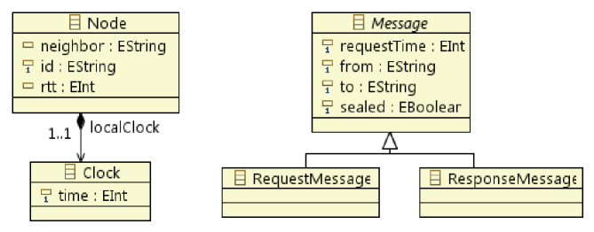
Figure 1: Abstract syntax of the round trip protocol language.

We have two kinds of messages, RequestMessage and ResponseMessage, that are subclasses of the generic Message class. A message contains a requestTime attribute denoting the time stamp, and to and from attributes denoting, respectively, the receiver and sender of the message. When a message is created, it is “sealed,” and the message can only be read when the seal has been removed; this models message delays as explained below.

The concrete syntax for the round trip time protocol language that assigns a graphical object to each class in the abstract syntax is given in Figure 2.

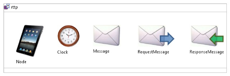
Figure 2: A concrete syntax for the round trip time protocol language.

The real-time behavior of the DSML can now specified by a set of visual model transformation rules.

Figure 3 shows the Request rule, which starts a round of the protocol for a node n. It models how the node n creates a request message m to its neighbor. The message is initially sealed, and includes the time of its creation (given by the node’s local clock). We consider that the action is instantaneous, and therefore the rule’s duration is set to the interval [0,0].

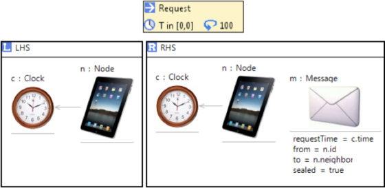
Figure 3: The Request periodic rule.

This is periodic rule, with period 100 (notice the loop icon in the header of the rule). Remember that, unless the rule is soft, an execution of a rule is scheduled as soon as possible for each set of objects that matches a rule’s left-hand side. Therefore, the above rule will be applied every 100 time units for each Node.

Successful message transmission is modeled by the Transfer rule shown in Figure 4.

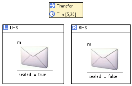
Figure 4: The Transfer atomic rule.

This action takes between five and twenty time units, and removes the seal of a message, which indicates that the message can be received. Any kind of message may get lost at any time, what is modeled by the Lost rule in Figure 5.

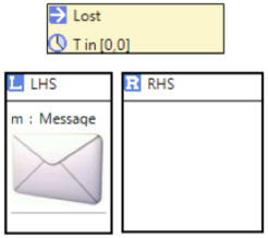
Figure 5: The Lost atomic rule.

Figure 6 shows the instantaneous atomic rule that applies when the seal of a request message m1 has been removed; that is, the message is ready to be received. The intended recipient n then consumes the message and sends a new (sealed) response message to the sender of the request message. This new message also includes the same time stamp that was received in the request message.

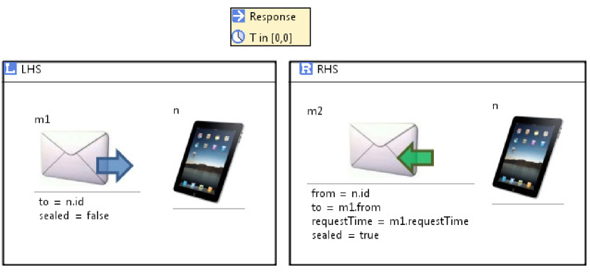
Figure 6: The Response instantaneous rule.

When the response message is received, the instantaneous rule ComputeRtt in Figure 7 computes the receiver’s rtt value by subtracting the time stamp m.requestTime from the current value of its local clock.

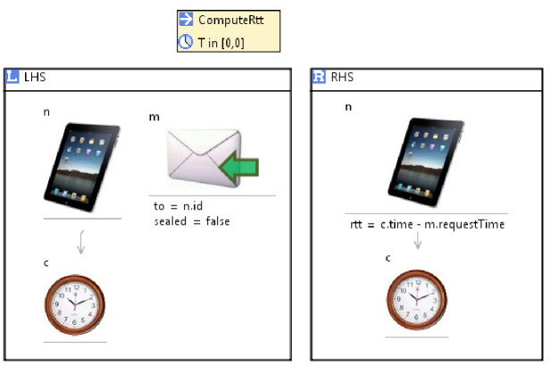
Figure 7: The ComputeRtt instantaneous rule.

Finally, the ongoing (notice the purple arrow) rule LocalTimeElapse, shown in Figure 8, increases the time value of each clock in the system by the elapsed time T.

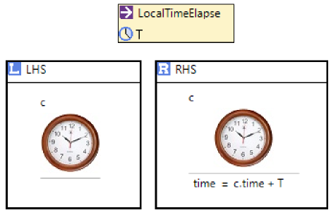
Figure 8: The LocalTimeElapse ongoing rule.

3.3 Formal Analysis of the Protocol

Let the model shown in Figure 9 be the initial model of the system. This model is composed of two nodes and their local clocks.

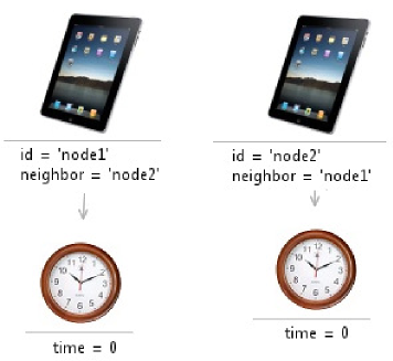
Figure 9: The rttpModel initial model.

Since a message transmission can take anywhere between five and twenty time units, we could expect that the round trip times will range between ten and forty time units. This property can easily be checked using the Maude’s search command. This command allows us to explore (following a breadth-first strategy) the reachable state space in different ways. Thus, we move to the Maude environment, and check if a model with a node whose rtt attribute is set to a value lower than ten time units or greater than forty time units can be reached:

⬇

search [1] init(rttpModel) =>* { MODEL:@Model } in time T:Time

such that << Node@rttp . allInstances

-> exists ( n | (n . rtt@OCLSf > 40) or (n . rtt@OCLSf < 10)) ;

MODEL:@Model >> .

No solution.

With this command, we are looking for a model MODEL that satisfies the condition expressed as an OCL expression in the such that clause as explained in Section 2. In this case, the search command does not find any solution, and therefore we can conclude that starting from our initial model, the round-trip time value of every node will always range between ten and forty time units.

We can also check whether the local clocks of the system are always synchronized by searching for a state that does not satisfy it, i.e., by looking for a state on which two clocks have different time values:

⬇

search [1] init(rttpModel) =>* { MODEL:@Model } in time T:Time

such that << ’clock1 . time@OCLSf <> ’clock2 . time@OCLSf ; MODEL:@Model >> .

No solution.

4 Earliest Deadline First Scheduling

This section explains how we can visually specify and formally analyze the well known earliest deadline first (EDF) scheduling algorithm in e-Motions. Even though model checking is not necessary to decide schedulability of this simple protocol, for much more complex scheduling algorithms where schedulability is very hard to analyze analytically, Real-Time Maude model checking analyses can indeed be successfully applied to analyze schedulability [7].

4.1 The EDF Scheduling Algorithm

In EDF scheduling with periodic tasks (see, e.g., [3]), we are given one or more processors and a set of tasks $\tau_{1},\ldots,\tau_{n}$, where each task $\tau_{i}$ is served by a constant bandwidth server $S_{i}$ with period $p_{i}$ and execution time $e_{i}$. The server $S_{i}$ executes the instances of $\tau_{i}$ in rounds of length $p_{i}$, and in each round it must have access to a/the processor for time $e_{i}$ in total.

Tasks can be preempted (i.e., suspended in the middle of an execution to allow the processor to execute tasks with higher priority), and it is always the task(s) with the earliest deadline that have the highest priority. That is, it is always the server with the least amount of time remaining of its current round that should be executing (unless it has ended its execution in the round).

Therefore, in EDF, the behavior of a server $S_{i}$ can be summarized as follows:

• At the beginning of each round: if a processor is idle, the server starts executing on the processor; if a processor is not idle, but the time until the end of the executing server $S_{j}$’s current round is greater than the period $p_{i}$, then $S_{i}$ preempts (and suspends) $S_{j}$ and starts executing; otherwise, the server $S_{i}$ starts waiting for an available processor.

• A waiting or suspended server may start executing when another server stops executing, and there are no other waiting/suspended servers with higher priority.

• When the server $S_{i}$ has executed for a total amount of time $e_{i}$ in its current round, it releases the processor, to the waiting/suspended server (if any) with the highest priority.

• When a server’s round ends, it immediately starts a new round.

4.2 Specifying EDF in e-Motions

The class diagram defining the abstract syntax of the DSML specifying the EDF algorithm is given in Figure 10.

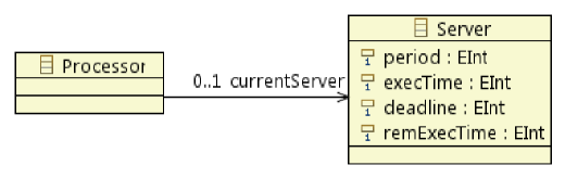
Figure 10: The EDF metamodel.

In this metamodel, a system is composed of a set of servers and a set of processors. A processor can execute at most a server at a time (see the currentServer reference). Task servers are identified by their period (attribute period) and their execution time (attribute execTime). The deadline and remExecTime attributes denote, respectively, the time until the end of the current round and the remaining execution time in the current round. The visual concrete syntax we have defined for the EDF example is shown in Figure 11.

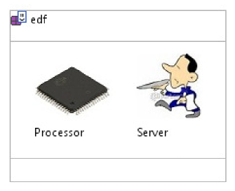
Figure 11: A concrete syntax for the EDF language.

The model transformation rules in Figures 12-16 define the dynamic behavior of EDF.

When the current round is over (i.e, the time remaining until the deadline is 0), the server s starts a new round by first setting its deadline attribute to the length of its period, and by setting the value of its remExecTime attribute, that denotes the remaining execution time of the new round, to whatever what left of the execution time in the previous round plus the execution time needed in this round. This is modeled by the instantaneous atomic model transformation rule NewPeriod in Figure 12.

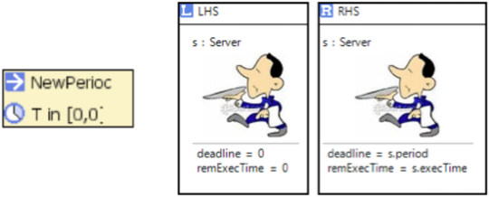
Figure 12: The NewPeriod instantaneous rule.

As already mentioned, unless an atomic rule is declared to be soft, it is applied as soon as it becomes enabled.

In the instantaneous atomic rule ServerSelection, shown in Figure 13, the server s gets to execute if there is no other server with remaining execution in the period with earlier deadline, and the currently executing server (if any) has a strictly later deadline than s.

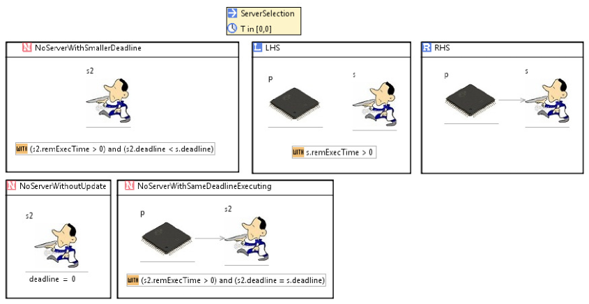
Figure 13: The ServerSelection instantaneous rule.

The rule ServerSelection also applies when a server s2 finishes its execution in a round, if there is a waiting/suspended server. The case when a server s finishes its execution (i.e., s.remExecTime is 0), but there is no server waiting, is modeled by the instantaneous atomic rule ReleaseProcessor in Figure 14, where s just releases the server at the end of its current execution if no server is waiting.

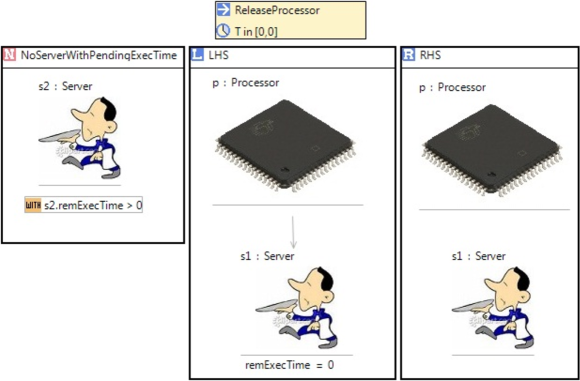
Figure 14: The ReleaseProcessor instantaneous rule.

Finally, we have two ongoing rules: Rule Execution in Figure 15 decreases the remaining deadline of each server according to the elapsed time T, until the node reaches the end of its round, and the rule DecreaseDeadline in Figure 16 decreases the remaining execution time of each executing server according to the elapsed time.

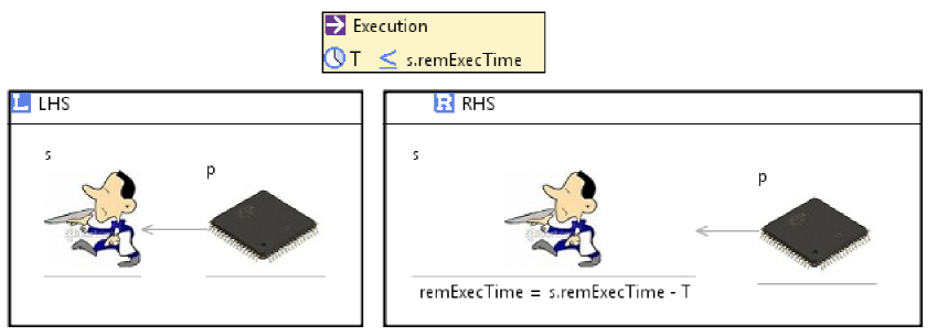
Figure 15: The Execution ongoing rule.

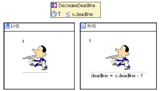
Figure 16: The DecreaseDeadline ongoing rule.

4.3 Analyzing the EDF Algorithm

We can use the generated Maude specification of the EDF language to analyze whether a given set of servers is schedulable; that is, whether all servers can execute for the allocated execution time execTime in each round.

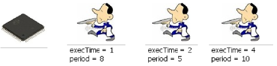
Figure 17: The edfModel initial model.

Figure 17 shows an initial model edfModel with three servers and one processors. To analyze whether this server set is schedulable, we search for a reachable model which can not execute for the desired amount of time in some round; that is, a model in which the remaining execution time is greater than the deadline for some server s:

⬇

search [1] init(edfModel) =>* { MODEL:@Model } in time T:Time

such that << Server@edf . allInstances

-> exists ( s | s . deadline@OCLSf < s . remExecTime@OCLSf ) ; MODEL:@Model >> .

5 Concluding Remarks

We have shown how two fairly small, but “non-artificial,” real-time systems in very different domains can be specified in the visual model transformation framework e-Motions. We have also shown how the Maude tool can be used to formally analyze the automatically synthesized Maude models. We leave it up to the reader to evaluate the convenience of using e-Motions for the specification and analysis of real-time systems, and also encourage her to compare this work with the specification and analysis of the same round trip example in the timed model transformation framework MOMENT2 [2].

Our personal impression is that it seems quite convenient to model systems in this way; however, the analysis support could be better integrated within e-Motions, despite the very significant advantage of having the <<_;_>> operator, which allows us to easily define any reachability and LTL model checking query without knowing anything about the internal Maude representation of our system.

References

- [1]
- [2] A. Boronat & P. C. Ölveczky (2010): Formal Real-Time Model Transformations in MOMENT2. In David S. Rosenblum & Gabriele Taentzer, editors: Proc. of the 13th International Conference on Fundamental Approaches to Software Engineering (FASE’10), Lecture Notes in Computer Science 6013, Springer, pp. 29–43. Available at http://dx.doi.org/10.1007/978-3-642-12029-9.
- [3] G. C. Buttazzo (2004): Hard Real-Time Computing Systems. Kluwer Academic Publishers.
- [4] M. Clavel, F. Durán, S. Eker, P. Lincoln, N. Martí-Oliet, J. Meseguer & C. Talcott (2007): All About Maude - A High-Performance Logical Framework. Lecture Notes in Computer Science 4350, Springer.
- [5] K. Czarnecki & S. Helsen (2003): Classification of Model Transformation Approaches. In: OOPSLA’03 Workshop on Generative Techniques in the Context of Model-Driven Architecture.
- [6] J. de Lara & H. Vangheluwe (2004): Defining Visual Notations and Their Manipulation Through Meta-Modelling and Graph Transformation. Journal of Visual Languages and Computing 15(3–4), pp. 309–330. Available at http://dx.doi.org/10.1016/j.jvlc.2004.01.005.
- [7] P. C. Ölveczky & M. Caccamo (2006): Formal Simulation and Analysis of the CASH Scheduling Algorithm in Real-Time Maude. In Luciano Baresi & Reiko Heckel, editors: Fundamental Approaches to Software Engineering, 9th International Conference, FASE 2006, Held as Part of the Joint European Conferences on Theory and Practice of Software, ETAPS 2006, Vienna, Austria, March 27-28, 2006, Proceedings, Lecture Notes in Computer Science 3922, Springer, pp. 357–372. Available at http://dx.doi.org/10.1007/11693017_26.
- [8] P. C. Ölveczky & J. Meseguer (2008): The Real-Time Maude Tool. In C. R. Ramakrishnan & Jakob Rehof, editors: Proc. TACAS’08, Lecture Notes in Computer Science 4963, Springer, pp. 332–336. Available at http://dx.doi.org/10.1007/978-3-540-78800-3_23.
- [9] J. E. Rivera (2010): On the Semantics of Real-Time Domain Specific Modeling Languages. Ph.D. thesis, Universidad de Málaga.
- [10] J. E. Rivera, F. Durán & A. Vallecillo (2009): A graphical approach for modeling time-dependent behavior of DSLs. In: IEEE Symposium on Visual Languages and Human-Centric Computing, VL/HCC 2009, Corvallis, OR, USA, 20-24 September 2009, Proceedings, IEEE, pp. 51–55. Available at http://doi.ieeecomputersociety.org/10.1109/VLHCC.2009.5295300%.
- [11] J. E. Rivera, F. Durán & A. Vallecillo (2010): On the Behavioral Semantics of Real-Time Domain Specific Visual Languages. In: Proc. WRLA’10, Lecture Notes in Computer Science 6381, Springer. See also the e-Motions web page http://atenea.lcc.uma.es/E-motions.
- [12] J. E. Rivera, E. Guerra, J. de Lara & A. Vallecillo (2008): Analyzing Rule-Based Behavioral Semantics of Visual Modeling Languages with Maude. In Dragan Gasevic, Ralf Lämmel & Eric Van Wyk, editors: Software Language Engineering, First International Conference, SLE 2008, Toulouse, France, September 29-30, 2008. Revised Selected Papers, Lecture Notes in Computer Science 5452, Springer, pp. 54–73. Available at http://dx.doi.org/10.1007/978-3-642-00434-6_5.
- [13] J. E. Rivera, A. Vallecillo & F. Durán (2009): Formal Specification and Analysis of Domain Specific Languages using Maude. Simulation: Transactions of the Society for Modeling and Simulation International 85(11/12), pp. 778–792. Available at http://dx.doi.org/10.1177/0037549709341635.
- [14] SAE AADL Team (2009): AADL Homepage. http://www.aadl.info/.
- [15] J. Troya, J. E. Rivera & A. Vallecillo (2010): Simulating Domain Specific Visual Models by Observation. In Robert M. McGraw, Eric S. Imsand & Michael J. Chinni, editors: Proceedings of the 2010 Spring Simulation Multiconference, SpringSim 2010, Orlando, Florida, USA, April 11-15, 2010, SCS/ACM, pp. 46–53. Available at http://doi.acm.org/10.1145/1878537.1878671.