Coherent vortex structures and 3D enstrophy cascade

Abstract.

Existence of 2D enstrophy cascade in a suitable mathematical setting, and under suitable conditions compatible with 2D turbulence phenomenology, is known both in the Fourier and in the physical scales. The goal of this paper is to show that the same geometric condition preventing the formation of singularities – $\frac{1}{2}$-Hölder coherence of the vorticity direction – coupled with a suitable condition on a modified Kraichnan scale, and under a certain modulation assumption on evolution of the vorticity, leads to existence of 3D enstrophy cascade in physical scales of the flow.

1. Introduction

The vorticity-velocity formulation of the 3D Navier-Stokes equations (NSE) reads

(1.1) $$\partial_{t}\omega+(u\cdot\nabla)\omega=(\omega\cdot\nabla)u+\triangle\omega$$

where $u$ is the velocity and $\omega=\,\mbox{curl}\,u$ is the vorticity of the fluid (the viscosity is set to 1). A comprehensive introduction to the mathematical study of the vorticity can be found in [MB02].

In 2D, the vortex-stretching term, $(\omega\cdot\nabla)u$, is identically zero, and the nonlinearity is simply a part of the transport of the vorticity by the flow.

This allowed the authors to adopt to 2D a general mathematical setting for the study of turbulent cascades and locality in physical scales of 3D incompressible viscous and inviscid flows introduced in [DaGr11-1] and [DaGr11-2], respectively, to establish existence of the enstrophy cascade and locality in 2D [DaGr11-3].

Since the vortex-stretching term is not a flux-type term, the only way to establish existence of the enstrophy cascade in 3D in this setting is to show that its contribution to the ensemble averaging process can be suitably interpolated between integral-scale averages of the enstrophy and the enstrophy dissipation rate.

This is where coherent vortex structures come into play. A role of the coherent vortex structures in turbulent flows was recognized as early as the 1500’s in Leonardo da Vinci’s “deluge” drawings. On the other hand, Kolmogorov’s K41 phenomenology [Ko41-1, Ko41-2] does not discern geometric structures; the K41 eddies are essentially amorphous. As stated by Frisch in his book Turbulence, The Legacy of A.N. Kolmogorov [Fr95], “Half a century after Kolmogorov’s work on the statistical theory of fully developed turbulence, we still wonder how his work can be reconciled with Leonardo’s half a millennium old drawings of eddy motion in the study for the elimination of rapids in the river Arno.” This remark was followed by a discussion on dynamical role, as well as statistical signature of vortex filaments in turbulent flows. Several (by now classical) directions in the study of the vortex dynamics of turbulence – both in 2D and 3D – are presented in Chorin’s book Vorticity and Turbulence (cf. [Ch94] and the references therein). The approach exposed in [Ch94] is essentially discrete (probabilistic lattice models); on the other hand, the first rigorous continuous statistical theory of vortex filaments was given by P.-L. Lions and Majda in [LM00].

Local anisotropic behavior of the enstrophy, i.e., self-organization of the regions of high vorticity in coherent vortex structures – most notably vortex filaments/tubes – is ubiquitous. In particular, local alignment or anti-alignment of the vorticity direction, i.e. local coherence, is prominently featured in turbulent flows. A strong numerical evidence, as well as several theoretical arguments explaining the physical mechanism behind the formation of coherent structures – including rigorous estimates on the flow directly from the 3D NSE – can be found, e.g., in [Co90, SJO91, CPS95, GGH97, GFD99, Oh09, GM11]. One way to look at the phenomenon of local coherence of the vorticity direction is to interpret it as a manifestation of the general observation that the regions of high fluid intensity are – in the vorticity formulation – locally ‘quasi 2D-like’ (in 2D, the vorticity direction is globally parallel or antiparallel).

The rigorous study of geometric depletion of the nonlinearity in the 3D NSE was pioneered by Constantin when he derived a singular integral representation for the stretching factor in the evolution of the vorticity magnitude featuring a geometric kernel depleted by coherence of the vorticity direction (cf. [Co94]). This was followed by the paper [CoFe93] where Constantin and Fefferman showed that as long as the vorticity direction in the regions of intense vorticity is Lipschitz-coherent, no finite-time blow up can occur, and later by the paper [daVeigaBe02] where Beirao da Veiga and Berselli scaled the coherence strength needed to deplete the nonlinearity down to $\frac{1}{2}$-Hölder.

A full spatiotemporal localization of the vorticity formulation of the 3D NSE was developed by one of the authors and the collaborators in [GrZh06, Gr09, GrGu10-1, GrGu10-2]. The main obstacle to the full localization of the evolution of the enstrophy was the spatial localization of the vortex-stretching term, $(\omega\cdot\nabla)u$. An explicit local representation for the vortex-stretching term was given in [Gr09], and the leading order term reads

(1.2) $$P.V.\int_{B(x_{0},2R)}\epsilon_{jkl}\frac{\partial^{2}}{\partial x_{i}\partial y_{k}}\frac{1}{|x-y|}\phi(y,t)\omega_{l}(y,t)\,dy\ \phi(x,t)\omega_{i}(x,t)\omega_{j}(x,t)$$

where $\epsilon_{jkl}$ is the Levi-Civita symbol and $\phi$ is a spatiotemporal cut-off associated with the ball $B(x_{0},R)$. The key feature of (1.2) is that it displays both analytic (via a local non-homogeneous Div-Curl Lemma [GrGu10-2]) and geometric (via coherence of the vorticity direction [Gr09, GrGu10-1]) cancelations, inducing analytic and geometric local depletion of the nonlinearity in the 3D vorticity model. (For a different approach to localization of the vorticity-velocity formulation see [ChKaLe07].)

The present work is envisioned as a contribution to the effort of understanding the role that the geometry of the flow and in particular, coherent vortex structures, plays in the theory of turbulent cascades. More precisely, we show – utilizing the aforementioned localization within the general mathematical framework for the study of turbulent cascades in physical scales of incompressible flows introduced in [DaGr11-1] (in this case, via suitable ensemble-averaging of the local enstrophy equality) – that coherence of the vorticity direction, coupled with a suitable condition on a modified Kraichnan scale, and under a certain modulation assumption on evolution of the vorticity, leads to existence of 3D enstrophy cascade in physical scales of the flow. This furnishes a mathematical evidence that, in contrast to 3D energy cascade, 3D enstrophy cascade is locally anisotropic, providing a form of a reconciliation between Leonardo’s and Kolmogorov’s views on turbulence on the enstrophy level.

It is worth pointing out that our theory of turbulent cascades in physical scales of 3D incompressible flows is on the energy level [DaGr11-1, DaGr11-2, DaGr12-1] consistent both with the K41 theory of turbulence and the Onsager’s predictions on existence of the inviscid energy cascade (and consequently, with the phenomena of anomalous dissipation and dissipation anomaly), as well as with the previous rigorous mathematical work on existence of the energy cascade in the wavenumbers [FMRT01]. In particular, on the energy level, it does not ‘see’ geometric structures. It is only here, i.e., on the enstrophy level, that the role of coherent vortex structures is revealed. A distinctive feature of our theory that makes incorporating the geometry of the flow and in particular, local coherence possible is the fact that the cascade takes place in the actual physical scales of the flow. To the best of our knowledge, there is nothing in the K41 theory that would contradict existence of the 3D enstrophy cascade; on the other hand, given that K41 takes place primarily in the Fourier space, i.e., in the wavenumbers, formulating conditions (within K41) faithfully reflecting various geometric properties of the flow is a much more challenging enterprise.

The paper is organized as follows. Section 2 recalls the ensemble-averaging process introduced in [DaGr11-1], and Section 3 the spatiotemporal localization of the evolution of the enstrophy developed in [GrZh06, Gr09, GrGu10-1, GrGu10-2]. Existence and locality of anisotropic 3D enstrophy cascade is presented in Section 4.

2. Ensemble averages

In studying a PDE model, a natural way of actualizing a concept of scale is to measure distributional derivatives of a quantity with respect to the scale. Let $x_{0}$ be in $B(0,R_{0})$ ($R_{0}$ being the integral scale, $B(0,2R_{0})$ contained in $\Omega$ where $\Omega$ is the global spatial domain) and $0<R\leq R_{0}$. Considering a locally integrable physical density of interest $f$ on a ball of radius $2R$, $B(x_{0},2R)$, a local physical scale $R$ – associated to the point $x_{0}$ – is realized via bounds on distributional derivatives of $f$ where a test function $\psi$ is a refined – smooth, non-negative, equal to 1 on $B(x_{0},R)$ and featuring optimal bounds on the derivatives over the outer $R$-layer – cut-off function on $B(x_{0},2R)$. More explicitly,

(2.1) $$|(D^{\alpha}f,\psi)|\leq\int_{B(x_{0},2R)}|f||D^{\alpha}\psi|\leq\Bigl{(}c(\alpha)\frac{1}{R^{|\alpha|}}|f|,\psi^{\delta(\alpha)}\Bigr{)}$$

for some $c(\alpha)>0$ and $\delta(\alpha)$ in $(0,1)$. (This is reminiscent of Bernstein inequalities in the Littlewood-Paley decomposition of a tempered distribution.)

Henceforth, we utilize refined spatiotemporal cut-off functions $\phi=\phi_{x_{0},R,T}=\psi\,\eta$, where $\eta=\eta_{T}(t)\in C^{\infty}(0,T)$ and $\psi=\psi_{x_{0},R}(x)\in\mathcal{D}(B(x_{0},2R))$ satisfying

(2.2) $$0\leq\eta\leq 1,\quad\eta=0\ \mbox{on}\ (0,T/3),\quad\eta=1\ \mbox{on}\ (2T/3,T),\quad\frac{|\eta^{\prime}|}{\eta^{\rho_{1}}}\leq\frac{C_{0}}{T}\;$$

and

(2.3) $$0\leq\psi\leq 1,\quad\psi=1\ \mbox{on}\ B(x_{0},R),\quad\frac{|\nabla\psi|}{\psi^{\rho_{2}}}\leq\frac{C_{0}}{R},\quad\frac{|\triangle\psi|}{\psi^{2\rho_{2}-1}}\leq\frac{C_{0}}{R^{2}}\;,$$

for some $\frac{1}{2}<\rho_{1},\rho_{2}<1$.

In particular, $\phi_{0}=\psi_{0}\eta$ where $\psi_{0}$ is the spatial cut-off (as above) corresponding to $x_{0}=0$ and $R=R_{0}$.

For $x_{0}$ near the boundary of the integral domain, $S(0,R_{0})$, we assume additional conditions,

(2.4) $$0\leq\psi\leq\psi_{0}$$

and, if $B(x_{0},R)\not\subset B(0,R_{0})$, then $\psi\in\mathcal{D}(B(0,2R_{0}))$ with $\psi=1\ \mbox{on}\ B(x_{0},R)\cap B(0,R_{0})$ satisfying, in addition to (2.3), the following:

(2.5) $$\psi=\psi_{0}\ \mbox{on the part of the cone centered at zero and passing through}$$

$$S(0,R_{0})\cap B(x_{0},R)\ \mbox{between}\ S(0,R_{0})\ \mbox{and}\ S(0,2R_{0})$$

and

(2.6) $$\psi=0\ \mbox{on}\ B(0,R_{0})\setminus B(x_{0},2R)\ \mbox{and outside the part of the cone}$$

$$\mbox{centered at zero and passing through}\ S(0,R_{0})\cap B(x_{0},2R)$$

$$\mbox{between}\ S(0,R_{0})\ \mbox{and}\ S(0,2R_{0}).$$

A physical scale $R$ – associated to the integral domain $B(0,R_{0})$ – is realized via suitable ensemble-averaging of the localized quantities with respect to ‘$(K_{1},K_{2})$-covers’ at scale $R$.

Let $K_{1}$ and $K_{2}$ be two positive integers, and $0<R\leq R_{0}$. A cover $\{B(x_{i},R)\}_{i=1}^{n}$ of the integral domain $B(0,R_{0})$ is a $(K_{1},K_{2})$-cover at scale $R$ if

$$\biggl{(}\frac{R_{0}}{R}\biggr{)}^{3}\leq n\leq K_{1}\biggr{(}\frac{R_{0}}{R}\biggr{)}^{3},$$

and any point $x$ in $B(0,R_{0})$ is covered by at most $K_{2}$ balls $B(x_{i},2R)$. The parameters $K_{1}$ and $K_{2}$ represent the maximal global and local multiplicities, respectively.

For a physical density of interest $f$, consider time-averaged, per unit mass – spatially localized to the cover elements $B(x_{i},R)$ – local quantities $\hat{f}_{x_{i},R}$,

$$\hat{f}_{x_{i},R}=\frac{1}{T}\int_{0}^{T}\frac{1}{R^{3}}\int_{B(x_{i},2R)}f(x,t)\phi^{\delta}_{x_{i},R,T}(x,t)\,dx\,dt$$

for some $0<\delta\leq 1$, and denote by $\langle F\rangle_{R}$ the ensemble average given by

$$\langle F\rangle_{R}=\frac{1}{n}\sum_{i=1}^{n}\hat{f}_{x_{i},R}\,.$$

The key feature of the ensemble averages $\{\langle F\rangle_{R}\}_{0<R\leq R_{0}}$ is that $\langle F\rangle_{R}$ being stable, i.e., nearly-independent on a particular choice of the cover (with the fixed parameters $K_{1}$ and $K_{2}$), indicates there are no significant fluctuations of the sign of the density $f$ at scales comparable or greater than $R$. On the other hand, if $f$ does exhibit significant sign-fluctuations at scales comparable or greater than $R$, suitable rearrangements of the cover elements up to the maximal multiplicities – emphasizing first the positive and then the negative parts of the function – will result in $\langle F\rangle_{R}$ experiencing a wide range of values, from positive through zero to negative, respectively.

Consequently, for an a priori sign-varying density, the ensemble averaging process acts as a coarse detector of the sign-fluctuations at scale $R$. (The larger the maximal multiplicities $K_{1}$ and $K_{2}$, the finer detection.)

As expected, for a non-negative density $f$, all the averages are comparable to each other throughout the full range of scales $R$, $0<R\leq R_{0}$; in particular, they are all comparable to the simple average over the integral domain. More precisely,

(2.7) $$\frac{1}{K_{*}}F_{0}\leq\langle F\rangle_{R}\leq K_{*}F_{0}$$

for all $0<R\leq R_{0}$, where

$$F_{0}=\frac{1}{T}\int\frac{1}{R_{0}^{3}}\int f(x,t)\phi_{0}^{\delta}(x,t)\,dx\,dt,$$

and $K_{*}=K_{*}(K_{1},K_{2})>1$.

There are several properties of the ensemble averaging process that although being plausible, deserve a precise analytic description/quantification. Besides the above statement on non-negative densities, perhaps the most elemental one is that if the averages at a certain scale are nearly independent of a particular choice of a $(K_{1},K_{2})$-cover ($K_{1}$ and $K_{2}$ fixed), then essentially the same universality property should propagate to larger scales. In order to obtain a precise quantitative propagation result, the universality is assumed on an initial interval, rather than at a single scale (this is due to the presence of smooth cut-offs with prescribed rates of change). Two types of results are presently available.

Let $f$ be a locally integrable function (a density), and $K_{1}$ and $K_{2}$ two positive integers.

TYPE I.  Assume that there exists $R_{*}>0$ such that for any $R$ in $[R^{*},2R_{*})$ and any $(27K_{1},16K_{2})$-cover at scale $R$, the averages $\langle F\rangle_{R}$ are all comparable to some value $F_{*}$; more precisely, $\displaystyle{\frac{1}{C_{1}}F_{*}\leq\langle F\rangle_{R}\leq C_{1}F_{*}}$. Then, for all $R\geq 2R_{*}$ and all $(K_{1},K_{2})$-covers at scale $R$, the averages $\langle F\rangle_{R}$ satisfy $\displaystyle{\frac{1}{C_{2}}F_{*}\leq\langle F\rangle_{R}\leq C_{2}F_{*}}$.

TYPE II.  Assume that there exists $R_{*}>0$ such that for any $R$ in $(\frac{1}{2}R^{*},\frac{5}{2}R_{*})$ and any $(K_{1},K_{2})$-cover at scale $R$, $\displaystyle{\frac{1}{C_{1}}F_{*}\leq\langle F\rangle_{R}\leq C_{1}F_{*}}$. Then, for all $R\geq\frac{5}{2}R_{*}$ and all $(K_{1},K_{2})$-covers at scale $R$, the averages $\langle F\rangle_{R}$ satisfy

$$\frac{1}{C_{3}}\Bigl{(}\frac{R_{*}}{R}\Bigr{)}^{C_{4}}F_{*}\leq\langle F\rangle_{R}\leq C_{3}\Bigl{(}\frac{R}{R^{*}}\Bigr{)}^{C_{4}}F_{*}.$$

Shortly, in a Type I result, the universality is assumed with respect to more refined covers, while in a Type II result, the non-exactness of the propagation caused by the smooth cut-offs is reflected in a correction to the universal value $F_{*}$ by the ratio of the scales $R$ and $R^{*}$.

The proofs are quite long and technical, and will be provided in a separate publication together with computational results describing the general statistics of the variation of the ensemble averages of multi-scale sign-fluctuating densities across the scales. Here, we provide a sample computation of the ensemble averages of a time-independent (to emphasize the spatial behavior) 1D density $f(x)=\cos^{2}(x+5)\sin\Bigl{(}\frac{1}{2}(x-1)^{2}\Bigr{)}$ (Figure 1), for $R_{0}=10$ and $K_{1}=K_{2}=3$; its global average is approximately $-0.003880$. The $y$-values in Figure 2 represent the ensemble averages with respect to the $(K_{1},K_{2})$-covers exhibiting maximal positive and negative bias, across the range of scales from $10^{-2}$ to $10^{1}=R_{0}$ (the $x$-values represent the powers of $10$); the red line slightly below the $x$-axis corresponds to the value of the global average. The response of the ensemble averages to sign-fluctuations at several different scales is clearly visible.

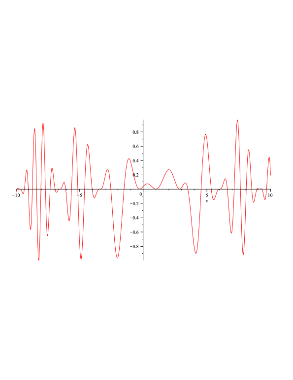
Figure 1. $f(x)=\cos^{2}(x+5)\sin\Bigl{(}\frac{1}{2}(x-1)^{2}\Bigr{)}$

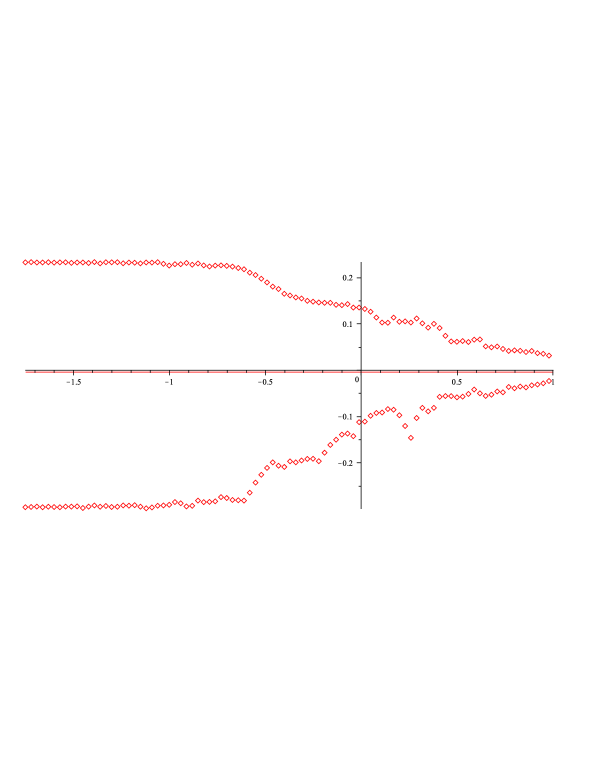
Figure 2. Ensemble averages with positive and negative bias.

3. Spatiotemporal localization of evolution of the enstrophy

The localization of the vorticity formulation introduced in [GrZh06, Gr09] was performed on an arbitrarily small parabolic cylinder below a point $(x_{0},t_{0})$ contained in the spatiotemporal domain $\Omega\times(0,T)$, with an eye on formulating the conditions preventing singularity formation at $(x_{0},t_{0})$. Here – in order to coordinate the notation with Section 2 – the localization will be performed on a spatiotemporal cylinder $B(x_{0},2R)\times(0,T)$ where $x_{0}$ belongs to the integral domain $B(0,R_{0})$ and $0<R\leq R_{0}$.

Suppose that the solution is smooth in $B(x_{0},2R)\times(0,T)$. Multiplying the equations by $\phi\,\omega$ ($\phi=\psi\eta$ being the cut-off introduced in Section 2) and integrating over $B(x_{0},2R)\times(0,t)$ for some $2T/3<t<T$ yields

$$\int\frac{1}{2}|\omega(x,t)|^{2}\psi(x)\;dx +\int_{0}^{t}\int|\nabla\omega|^{2}\phi\;dx\;ds$$

$$=\int_{0}^{t}\int\frac{1}{2}|\omega|^{2}(\phi_{t}+\triangle\phi)\;dx\;ds$$

(3.1) $$+\int_{0}^{t}\int\frac{1}{2}|\omega|^{2}(u\cdot\nabla\phi)\;dx\;ds+\int_{0}^{t}\int(\omega\cdot\nabla)u\cdot\phi\omega\;dx\;ds.$$

Suppressing the time variable, the localized vortex-stretching term can be written as (cf. [Gr09])

$$(\omega\cdot\nabla)u\cdot\phi\omega\,(x) =\phi^{\frac{1}{2}}(x)\,\frac{\partial}{\partial x_{i}}u_{j}(x)\,\phi^{\frac{1}{2}}(x)\,\omega_{i}(x)\,\omega_{j}(x)$$

$$=-c\,P.V.\int_{B(x_{0},2r)}\epsilon_{jkl}\,\frac{\partial^{2}}{\partial x_{i}\partial y_{k}}\frac{1}{|x-y|}\,\phi^{\frac{1}{2}}\,\omega_{l}\,dy\ \phi^{\frac{1}{2}}(x)\,\omega_{i}(x)\,\omega_{j}(x)+\ \mbox{LOT}$$

$$=-c\,P.V.\int_{B_{(}x_{0},2r)}\bigl{(}\omega(x)\times\omega(y)\bigr{)}\cdot G_{\omega}(x,y)\,\phi^{\frac{1}{2}}(y)\,\phi^{\frac{1}{2}}(x)\,dy+\ \mbox{LOT}$$

(3.2) $$=\ \mbox{VST}\ +\ \mbox{LOT}$$

where $\epsilon_{jkl}$ is the Levi-Civita symbol,

$$\bigl{(}G_{\omega}(x,y)\bigr{)}_{k}=\frac{\partial^{2}}{\partial x_{i}\partial y_{k}}\frac{1}{|x-y|}\,\omega_{i}(x)$$

and LOT denotes the lower order terms.

The above representation formula for the leading order vortex-stretching term VST features both analytic and geometric cancelations.

The geometric cancelations were utilized in [Gr09] to obtain a full localization of $\frac{1}{2}$-Hölder coherence of the vorticity direction regularity criterion, and then in [GrGu10-1] to introduce a family of scaling-invariant regularity classes featuring a precise balance between coherence of the vorticity direction and spatiotemporal integrability of the vorticity magnitude. Denote by $\xi$ the vorticity direction, and let $(x,t)$ be a spatiotemporal point, $r>0$ and $0<\gamma<1$. A $\gamma$-Hölder measure of coherence of the vorticity direction at $(x,t)$ is then given by

$$\rho_{\gamma,r}(x,t)=\sup_{y\in B(x,r),y\neq x}\frac{|\sin\varphi\bigl{(}\xi(x,t),\xi(y,t)\bigr{)}|}{|x-y|^{\gamma}}.$$

The following regularity class – a scaling-invariant improvement of $\frac{1}{2}$-Hölder coherence – is included,

(3.3) $$\int_{t_{0}-(2R)^{2}}^{t_{0}}\int_{B(x_{0},2R)}|\omega(x,t)|^{2}\ \rho^{2}_{\frac{1}{2},2R}(x,t)dx\,dt<\infty.$$

On the other hand, the analytic cancelations were utilized in [GrGu10-2] via a local non-homogeneous Div-Curl Lemma to obtain a full spatiotemporal localization of Kozono-Taniuchi generalization of Beale-Kato-Majda regularity criterion; namely, the time-integrability of the $BMO$ norm of the vorticity.

4. 3D enstrophy cascade

Let $\mathcal{R}$ be a region contained in the global spatial domain $\Omega$. The inward enstrophy flux through the boundary of the region is given by

$$-\int_{\partial\mathcal{R}}\frac{1}{2}|\omega|^{2}(u\cdot n)\,d\sigma=-\int_{\mathcal{R}}(u\cdot\nabla)\omega\cdot\omega\,dx$$

where $n$ denotes the outward normal (taking into account incompressibility of the flow). Localization of the evolution of the enstrophy to cylinder $B(x_{0},2R)\times(0,T)$ (cf. Section 3) leads to the following version of the enstrophy flux,

(4.1) $$\int\frac{1}{2}|\omega|^{2}(u\cdot\nabla\phi)\,dx=-\int(u\cdot\nabla)\omega\cdot\phi\omega\,dx$$

(again, taking into account the incompressibility; here, $\phi=\phi_{x_{0},R,T}$ defined in Section 2). Since $\nabla\phi=(\nabla\psi)\eta$, and $\psi$ can be constructed such that $\nabla\psi$ points inward – toward $x_{0}$ – (4.1) represents local inward enstrophy flux, at scale $R$ (more precisely, through the layer $S(x_{0},R,2R)$) around the point $x_{0}$. In the case the point $x_{0}$ is close to the boundary of the integral domain $B(0,R_{0})$, $\nabla\psi$ is not exactly radial, but still points inward.

Consider a $(K_{1},K_{2})$ cover $\{B(x_{i},R)\}_{i=1}^{n}$ at scale $R$, for some $0<R\leq R_{0}$. Local inward enstrophy fluxes, at scale $R$, associated to the cover elements $B(x_{i},R)$, are then given by

(4.2) $$\int\frac{1}{2}|\omega|^{2}(u\cdot\nabla\phi_{i})\,dx,$$

for $1\leq i\leq n$ ($\phi_{i}=\phi_{x_{i},R,T}$). Assuming smoothness, the identity (3) written for $B(x_{i},R)$ yields the following expression for time-integrated local fluxes,

$$\int_{0}^{t}\int\frac{1}{2}|\omega|^{2}(u\cdot\nabla\phi_{i})\;dx\;ds =\int\frac{1}{2}|\omega(x,t)|^{2}\psi_{i}(x)\;dx+\int_{0}^{t}\int|\nabla\omega|^{2}\phi_{i}\;dx\;ds$$

$$-\int_{0}^{t}\int\frac{1}{2}|\omega|^{2}\bigl{(}(\phi_{i})_{s}+\triangle\phi_{i}\bigr{)}\;dx\;ds$$

(4.3) $$-\int_{0}^{t}\int(\omega\cdot\nabla)u\cdot\phi_{i}\,\omega\;dx\;ds,$$

for any $t$ in $(2T/3,T)$ and $1\leq i\leq n$.

Denoting the time-averaged local fluxes per unit mass associated to the cover element $B(x_{i},R)$ by $\hat{\Phi}_{x_{i},R}$,

(4.4) $$\hat{\Phi}_{x_{i},R}=\frac{1}{t}\int_{0}^{t}\frac{1}{R^{3}}\int\frac{1}{2}|\omega|^{2}(u\cdot\nabla\phi_{i})\,dx,$$

the main quantity of interest is the ensemble average of $\{\hat{\Phi}_{x_{i},R}\}_{i=1}^{n}$ in the sense of Section 2; namely,

(4.5) $$\langle\Phi\rangle_{R}=\frac{1}{n}\sum_{i=1}^{n}\hat{\Phi}_{x_{i},R}.$$

Since the flux density, $-(u\cdot\nabla)\omega\cdot\omega$, is an a priori sign-varying density, the stability, i.e., the near-constancy of $\langle\Phi\rangle_{R}$ – while the ensemble averages are being run over all $(K_{1},K_{2})$ covers at scale $R$ – will indicate there are no significant sign-fluctuations of the flux density at the scales comparable or greater than $R$.

The main goal of this section is to formulate a set of physically reasonable conditions on the flow in $B(0,2R_{0})\times(0,T)$ implying the positivity and near-constancy of $\langle\Phi\rangle_{R}$ across a suitable range of scales – existence of the enstrophy cascade.

We will consider the case $\Omega=\mathbb{R}^{3}$. The main reason is that in the case of a domain with the boundary, it is necessary to utilize the full spatial localization (joint in $x$ and $y$) of the vortex-stretching term given by (3); this introduces a number of the lower order terms which – in turn – lead to terms of the form

$$c_{\gamma}\frac{1}{R^{\gamma}}\iint|\omega|^{2}\phi_{i}^{2\rho-1}\,dx\,ds$$

for some $\gamma>2$ ($c_{\gamma}$ is a suitable dimensional constant – scaling like $R^{\gamma-2}$). Such terms introduce a correction to the dissipation cut-off in the enstrophy cascade; namely, the modified Kraichnan scale $\sigma_{0}$ (see (A2) below) would have to be replaced by $\sigma_{0}^{\frac{2}{\gamma}}$ (times a dimensional constant). On the other hand, in $\mathbb{R}^{3}$, the full (spatial) localization of the vortex-stretching term can be replaced by the spatial localization in $x$ only,

(4.6) $$(\omega\cdot\nabla)u\cdot\phi_{i}\omega\,(x)=-c\,P.V.\int\bigl{(}\omega(x)\times\omega(y)\bigr{)}\cdot G_{\omega}(x,y)\,\phi_{i}^{\frac{1}{2}}(x)\,\phi_{i}^{\frac{1}{2}}(x)\;dy;$$

the $y$ integral is then split in suitable small and large scales (similarly to [GrZh06]) without introducing correction terms (cf. the proof of the main result in this section).

(A1)   Coherence Assumption

Denote the vorticity direction field by $\xi$, and let $M>0$ (large). Assume that there exists a positive constant $C_{1}$ such that

$$|\sin\varphi\bigl{(}\xi(x,t),\xi(y,t)\bigr{)}|\leq C_{1}|x-y|^{\frac{1}{2}}$$

for any $(x,y,t)$ in $\bigl{(}B(0,2R_{0})\times B(0,2R_{0}+R_{0}^{\frac{2}{3}})\times(0,T)\bigr{)}\cap\{|\nabla u|>M\}$ ($\varphi(z_{1},z_{2})$ denotes the angle between the vectors $z_{1}$ and $z_{2}$). Shortly, $\frac{1}{2}$-Hölder coherence in the region of intense fluid activity (large gradients).

Note that the previous local regularity results [GrZh06, Gr09] imply that – under (A1) – the a priori weak solution in view is in fact smooth inside $B(0,2R_{0})\times(0,T)$, and can, moreover, be smoothly continued (locally-in-space) past $t=T$; in particular, we can write (4) with $t=T$.

Let us briefly remark that in the aforementioned works on regularity, the region of intense fluid activity is usually defined as $\{|\omega|>M\}$ rather that $\{|\nabla u|>M\}$. Cutting-off at $|\omega|=M$ here would eventually lead to replacing $E_{0}$ in the definition of the modified Kraichnan scale $\sigma_{0}$ (see the next paragraph) by

$$E_{0}=\frac{1}{T}\int\frac{1}{R_{0}^{3}}\int\frac{1}{2}|\nabla u|^{2}\phi_{0}^{2\rho-1}\,dx\,dt,$$

and we prefer keeping $\sigma_{0}$ solely in terms of $\omega$.

(A2)   Modified Kraichnan Scale

Denote by $E_{0}$ time-averaged enstrophy per unit mass associated with the integral domain $B(0,2R_{0})\times(0,T)$,

$$E_{0}=\frac{1}{T}\int\frac{1}{R_{0}^{3}}\int\frac{1}{2}|\omega|^{2}\phi_{0}^{2\rho-1}\,dx\,dt,$$

by $P_{0}$ a modified time-averaged palinstrophy per unit mass,

$$P_{0}=\frac{1}{T}\int\frac{1}{R_{0}^{3}}\int|\nabla\omega|^{2}\phi_{0}\,dx\,dt+\frac{1}{T}\frac{1}{R_{0}^{3}}\int\frac{1}{2}|\omega(x,T)|^{2}\psi_{0}(x)\,dx$$

(the modification is due to the shape of the temporal cut-off $\eta$), and by $\sigma_{0}$ a corresponding modified Kraichnan scale,

$$\sigma_{0}=\biggl{(}\frac{E_{0}}{P_{0}}\biggr{)}^{\frac{1}{2}}.$$

Then, the assumption (A2) is simply a requirement that the modified Kraichnan scale associated with the integral domain $B(0,2R_{0})\times(0,T)$ be dominated by the integral scale,

$$\sigma_{0}<\beta R_{0},$$

for a constant $\beta$, $0<\beta<1$, $\beta=\beta(\rho,K_{1},K_{2},M,B_{T})$, where $\displaystyle{B_{T}=\sup_{t\in(0,T)}\|\omega(t)\|_{L^{1}}}$; this is finite provided the initial vorticity is a finite Radon measure [Co90].

(A3)   Localization and Modulation

The general set up considered is one of the weak Leray solutions satisfying (A1). As already mentioned, (A1) implies smoothness; however, the control on regularity-type norms is only local. On the other hand, the energy inequality on the global spatiotemporal domain $\mathbb{R}^{3}\times(0,T)$ implies

$$\int_{0}^{T}\int_{\mathbb{R}^{3}}|\omega|^{2}\,dx\,dt<\infty;$$

consequently, for a given constant $C_{2}>0$, there exists $R_{0}^{*}>0$ ($R_{0}^{*}\leq\min\{\sqrt{T},1\}$; this is mainly for convenience) such that

(4.7) $$\int_{0}^{T}\int_{B(0,2R_{0}+R_{0}^{\frac{2}{3}})}|\omega|^{2}\,dx\,dt\leq\frac{1}{C_{2}}$$

for any $0<R_{0}\leq R_{0}^{*}$. This is the localization assumption on $R_{0}$; the precise value of the constant $C_{2}$ is given in the proof of the theorem – right after the inequality (4).

The modulation assumption on the evolution of local enstrophy on $(0,T)$ – consistent with the choice of the temporal cut-off $\eta$ – reads

$$\int|\omega(x,T)|^{2}\psi_{0}(x)\,dx\geq\frac{1}{2}\sup_{t\in(0,T)}\,\int|\omega(x,t)|^{2}\psi_{0}(x)\,dx.$$

Remark 4.1.

Assumption (A1) is simply a quantification of the degree of local coherence of the vorticity direction – a manifestation of the local ‘quasi 2D-like’ behavior of turbulent flows – needed to sufficiently deplete the nonlinearity. Assumption (A2) is a slight modification of the condition implying existence of the enstrophy cascade in 2D (cf. [DaGr11-2]); namely, a requirement that the modified Kraichnan scale be dominated by the integral scale. Once unraveled, it postulates that the region of interest exhibits large vorticity gradients (relative to the vorticity magnitude, in the spatiotemporal average) – indicating high spatial complexity of the flow – and is the enstrophy analogue of the condition implying existence of the energy cascade in 3D ([DaGr11-1]), i.e., large velocity gradients (relative to the velocity magnitude, in the spatiotemporal average). The last assumption is somewhat technical; however, its purpose within our theory is physical – to prevent uncontrolled temporal fluctuations of $R_{0}$-scale enstrophy. Such fluctuations would inevitably prevent the cascade over $B(0,R_{0})$ (the region of interest).

Theorem 4.1.

Let $u$ be a Leray solution on $\mathbb{R}^{3}\times(0,T)$ with the initial vorticity $\omega_{0}$ being a finite Radon measure. Suppose that $u$ satisfies (A1)-(A3) on the spatiotemporal integral domain $B(0,2R_{0}+R_{0}^{\frac{2}{3}})\times(0,T)$. Then,

$$\frac{1}{4K_{*}}P_{0}\leq\langle\Phi\rangle_{R}\leq 4K_{*}\ P_{0}$$

for all $R,\,\frac{1}{\beta}\sigma_{0}\leq R\leq R_{0}$ ($K_{*}>1$ is the constant in (2.7)).

Proof.

Throughout the proof, $(K_{1},K_{2})$ cover parameters $\rho,K_{1}$ and $K_{2}$, as well as the gradient cut-off $M$ will be fixed. Henceforth, the quantities depending only on $\rho,K_{1},K_{2},M,B_{T}$ will be considered constants and denoted by a generic $K$ (that may change from line to line).

Let $0<R\leq R_{0}$. As already noted, we can write the expression for a time-integrated local flux corresponding to the cover element $B(x_{i},R)$, (4), for $t=T$,

$$\int_{0}^{T}\int\frac{1}{2}|\omega|^{2}(u\cdot\nabla\phi_{i})\;dx\;ds =\int\frac{1}{2}|\omega(x,T)|^{2}\psi_{i}(x)\;dx+\int_{0}^{T}\int|\nabla\omega|^{2}\phi_{i}\;dx\;ds$$

$$-\int_{0}^{T}\int\frac{1}{2}|\omega|^{2}\bigl{(}(\phi_{i})_{s}+\triangle\phi_{i}\bigr{)}\;dx\;ds$$

(4.8) $$-\int_{0}^{T}\int(\omega\cdot\nabla)u\cdot\phi_{i}\,\omega\;dx\;ds.$$

The last two terms on the right-hand side need to be estimated.

For the first term, the properties of the cut-off $\phi_{i}$ together with the condition $T\geq R_{0}^{2}\geq R^{2}$ yield

(4.9) $$\int_{0}^{T}\int\frac{1}{2}|\omega|^{2}\bigl{(}(\phi_{i})_{s}+\triangle\phi_{i}\bigr{)}\;dx\;ds\leq K\frac{1}{R^{2}}\int_{0}^{T}\int|\omega|^{2}\phi_{i}^{2\rho-1}\;dx\;ds.$$

For the second term, the vortex-stretching term

$$\int_{0}^{T}\int(\omega\cdot\nabla)u\cdot\phi_{i}\,\omega\;dx\;ds,$$

the integration is first split into the regions in which $|\nabla u|\leq M$ and $|\nabla u|>M$. In the first region, the integral is simply dominated by

(4.10) $$K\frac{1}{R^{2}}\int_{0}^{T}\int|\omega|^{2}\phi_{i}^{2\rho-1}\;dx\;ds$$

($R\leq R_{0}\leq 1$). In the second region, and for a fixed $x$, we divide the domain of integration in the representation formula (4.6),

$$(\omega\cdot\nabla)u\cdot\phi_{i}\omega\,(x)=-c\,P.V.\int\bigl{(}\omega(x)\times\omega(y)\bigr{)}\cdot G_{\omega}(x,y)\,\phi_{i}^{\frac{1}{2}}(x)\,\phi_{i}^{\frac{1}{2}}(x)\,dy,$$

into the regions outside and inside the sphere $\{y:\,|x-y|=R^{\frac{2}{3}}\}$. In the first case, the integral is bounded by

$$\iint_{\{|\nabla u|>M\}} \int_{\{y:\,|x-y|>R^{\frac{2}{3}}\}}\frac{1}{|x-y|^{3}}|\omega|\,dy\ \phi_{i}|\omega|^{2}\,dx\,ds$$

$$\leq K\frac{1}{R^{2}}\,\sup_{t}\,\|\omega(t)\|_{L^{1}}\int_{0}^{T}\int|\omega|^{2}\phi_{i}^{2\rho-1}\;dx\;ds$$

(4.11) $$\leq K\frac{1}{R^{2}}\int_{0}^{T}\int|\omega|^{2}\phi_{i}^{2\rho-1}\;dx\;ds.$$

In the second case – utilizing (A1), the Hardy-Littlewood-Sobolev and the Gagliardo-Nirenberg interpolation inequalities, and the localization part of (A3) – the following string of bounds transpires.

$$\iint_{\{|\nabla u|>M\}} \int_{\{y:\,|x-y|<R^{\frac{2}{3}}\}}\frac{1}{|x-y|^{\frac{5}{2}}}|\omega|\,dy\ \phi_{i}|\omega|^{2}\,dx\,ds$$

$$\leq K\int_{0}^{T}\|\omega\|_{L^{2}\bigl{(}B(x_{0},2R_{0}+R_{0}^{\frac{2}{3}})\bigr{)}}\|\,|\phi_{i}^{\frac{1}{2}}\omega|^{2}\,\|_{\frac{3}{2}}\,ds$$

$$\leq K\int_{0}^{T}\|\omega\|_{L^{2}\bigl{(}B(x_{0},2R_{0}+R_{0}^{\frac{2}{3}})\bigr{)}}\|\phi_{i}^{\frac{1}{2}}\omega\|_{2}\,\|\nabla(\phi_{i}^{\frac{1}{2}}\omega)\|_{2}\,ds$$

$$\leq K\ \biggl{(}\int_{0}^{T}\|\omega\|_{L^{2}\bigl{(}B(x_{0},2R_{0}+R_{0}^{\frac{2}{3}})\bigr{)}}^{2}\,ds\biggr{)}^{\frac{1}{2}}\,\biggl{(}\frac{1}{2}\sup_{t\in(0,T)}\|\psi_{i}^{\frac{1}{2}}\omega\|_{2}^{2}+\int_{0}^{T}\|\nabla(\phi_{i}^{\frac{1}{2}}\omega)\|_{2}^{2}\,ds\biggr{)}$$

$$\leq\frac{1}{8K_{*}^{2}}\ \biggl{(}\frac{1}{2}\sup_{t\in(0,T)}\|\psi_{i}^{\frac{1}{2}}\omega\|_{2}^{2}+\int_{0}^{T}\|\nabla(\phi_{i}^{\frac{1}{2}}\omega)\|_{2}^{2}\,ds\biggr{)},$$

where $K_{*}$ is the constant in (2.7) (in the last line, we used the localization assumption (4.7) with $C_{2}=64K^{2}K_{*}^{4}$). Incorporating the estimate

$$\int|\nabla(\phi_{i}^{\frac{1}{2}} \omega)|^{2}\,dx$$

$$\leq 2\int|\nabla\omega|^{2}\phi_{i}\,dx+c\int\biggl{(}\frac{|\nabla\phi_{i}|}{\phi_{i}^{\frac{1}{2}}}\biggr{)}^{2}\,|\omega|^{2}\,dx$$

$$\leq 2\int|\nabla\omega|^{2}\phi_{i}\,dx+K\frac{1}{R^{2}}\int|\omega|^{2}\phi_{i}^{2\rho-1}\,dx$$

in (4), we arrive at the final bound,

$$\iint_{\{|\nabla u|>M\}} \int_{\{y:\,|x-y|<R^{\frac{2}{3}}\}}\frac{1}{|x-y|^{\frac{5}{2}}}|\omega|\,dy\ \phi_{i}|\omega|^{2}\,dx\,ds$$

$$\leq\frac{1}{4K_{*}^{2}}\ \biggl{(}\frac{1}{2}\sup_{t\in(0,T)}\|\psi_{i}^{\frac{1}{2}}\omega\|_{2}^{2}+\int_{0}^{T}\|\nabla\omega\,\phi_{i}^{\frac{1}{2}}\|_{2}^{2}\,ds\biggr{)}+K\frac{1}{R^{2}}\int|\omega|^{2}\phi_{i}^{2\rho-1}\,dx.$$

Collecting the estimates (4.9)-(4) and using the modulation part of (A3), the relation (4) yields

$$\int_{0}^{T}\int\frac{1}{2}|\omega|^{2}(u\cdot\nabla\phi_{i})\;dx\;ds =\int\frac{1}{2}|\omega(x,T)|^{2}\psi_{i}(x)\;dx+\int_{0}^{T}\int|\nabla\omega|^{2}\phi_{i}\;dx\;ds\,+\,Z$$

where

$$Z\leq\frac{1}{2K_{*}^{2}}\ \biggl{(}\frac{1}{2}\|\psi_{i}^{\frac{1}{2}}(\cdot)\omega(\cdot,T)\|_{2}^{2}+\int_{0}^{T}\|\nabla\omega\,\phi_{i}^{\frac{1}{2}}\|_{2}^{2}\,ds\biggr{)}+K\frac{1}{R^{2}}\int|\omega|^{2}\phi_{i}^{2\rho-1}\,dx.$$

Taking the ensemble averages and exploiting (2.7) multiple times, we arrive at

$$\frac{1}{4K_{*}}P_{0}\leq\langle\Phi\rangle_{R}\leq 4K_{*}P_{0}$$

for all $\frac{1}{\beta}\sigma_{0}\leq R\leq R_{0}$, and a suitable $\beta=\beta(\rho,K_{1},K_{2},M,B_{T})$. ∎

Remark 4.2.

The first mathematical result on existence of 2D enstrophy cascade is in the paper by Foias, Jolly, Manley and Rosa [FJMR02]; the general setting is the one of infinite-time averages in the space-periodic case, and the cascade is in the Fourier space, i.e., in the wavenumbers. A recent work [DaGr11-3] provides existence of 2D enstrophy cascade in the physical space utilizing the general mathematical setting for the study of turbulent cascade in physical scales introduced in [DaGr11-1]. To the best of our knowledge, the present paper is the first rigorous result concerning existence of the enstrophy cascade in 3D.

The second theorem concerns locality of the flux. According to turbulence phenomenology, the average flux at scale $R$ – throughout the inertial range – is supposed to be well-correlated only with the average fluxes at nearby scales. In particular, the locality along the dyadic scale is expected to propagate exponentially.

Denoting the time-averaged local fluxes associated to the cover element $B(x_{i},R)$ by $\hat{\Psi}_{x_{i},R}$,

(4.16) $$\hat{\Psi}_{x_{i},R}=\frac{1}{T}\int_{0}^{T}\int\frac{1}{2}|\omega|^{2}(u\cdot\nabla\phi_{i})\,dx,$$

the (time and ensemble) averaged flux is given by

(4.17) $$\langle\Psi\rangle_{R}=\frac{1}{n}\sum_{i=1}^{n}\hat{\Psi}_{x_{i},R}=R^{3}\,\langle\Phi\rangle_{R}.$$

The following locality result is a simple consequence of the universality of the cascade of the time and ensemble-averaged local fluxes per unit mass $\langle\Phi\rangle_{R}$ obtained in Theorem 4.1.

Theorem 4.2.

Let $u$ be a Leray solution on $\mathbb{R}^{3}\times(0,T)$ with the initial vorticity $\omega_{0}$ being a finite Radon measure. Suppose that $u$ satisfies (A1)-(A3) on the spatiotemporal integral domain $B(0,2R_{0}+R_{0}^{\frac{2}{3}})\times(0,T)$, and let $R$ and $r$ be two scales within the inertial range delineated in Theorem 4.1. Then

$$\frac{1}{16K_{*}^{2}}\biggl{(}\frac{r}{R}\biggr{)}^{3}\leq\frac{\langle\Psi\rangle_{r}}{\langle\Psi\rangle_{R}}\leq 16K_{*}^{2}\biggl{(}\frac{r}{R}\biggr{)}^{3}.$$

In particular, if $r=2^{k}R$ for some integer $k$, i.e., through the dyadic scale,

$$\frac{1}{16K_{*}^{2}}\ 2^{3k}\leq\frac{\langle\Psi\rangle_{2^{k}R}}{\langle\Psi\rangle_{R}}\leq 16K_{*}^{2}\ 2^{3k}.$$

Remark 4.3.

Previous locality results include locality of the flux via a smooth filtering approach presented in [E05] (see also [EA09]), and locality of the flux in the Littlewood-Paley setting obtained in [CCFS08]. The aforementioned results are derived independently of existence of the inertial range, and are essentially kinematic upper bounds on the localized flux in terms of a suitable physical quantity localized to the nearby scales; the corresponding lower bounds hold assuming saturation of certain inequalities consistent with the turbulent behavior. In contrast, our result is derived dynamically as a direct consequence of existence of the turbulent cascade in view, and features comparable upper and lower bounds throughout the inertial range.

ACKNOWLEDGEMENTS  The authors thank an anonymous referee for a number of suggestions that lead to the present version of the paper. Z.G. acknowledges the support of the Research Council of Norway via the grant number 213473 - FRINATEK.

References

- [Ko41-1] A.N. Kolmogorov, Dokl. Akad. Nauk SSSR 30, 9 (1941).
- [Ko41-2] A.N. Kolmogorov, Dokl. Akad. Nauk SSSR 31, 538 (1941).
- [Co90] P. Constantin, Comm. Math. Phys 129, 241 (1990).
- [SJO91] Z.-S. She, E, Jackson and S. Orszag, Proc. R. Soc. Lond. A, 434, 101 (1991).
- [Co94] P. Constantin, SIAM Rev. 36, 73 (1994).
- [CoFe93] P. Constantin and C. Fefferman, Indiana Univ. Math. J. 42, 775 (1993).
- [Ch94] A. Chorin, Vorticity and Turbulence. Applied Mathematics Sciences 103, Springer-Verlag, 1994.
- [CPS95] P. Constantin, I. Procaccia and D. Segel, Phys. Rev. E, 51, 3207 (1995).
- [Fr95] U. Frisch, Turbulence. Cambridge University Press, 1995. The legacy of A.N. Kolmogorov.
- [GGH97] B. Galanti, J.D. Gibbon and M. Heritage, Nonlinearity 10, 1675 (1997).
- [GFD99] J.D. Gibbon, A.S. Fokas and C.R. Doering, Phys. D 132, 497 (1999).
- [LM00] P.-L. Lions and A. Majda, Comm. Pure Appl. Math. 53 76 (2000).
- [FMRT01] C. Foias, O. Manley, R. Rosa and R. Temam, C.R. Acad. Sci. Paris Sér. I Math. 333, 499 (2001).
- [MB02] A. Majda and A. Bertozzi, Vorticity and incompressible flow. Cambridge University Press, 2002.
- [FJMR02] C. Foias, M. Jolly, O. Manley, and R. Rosa, J. Stat. Phys. 108 591 (2002).
- [daVeigaBe02] H. Beirao da Veiga and L.C. Berselli, Diff. Int. Eqs. 15, 345 (2002).
- [E05] G. Eyink, Physica D 207, 91 (2005).
- [GrZh06] Z. Grujić and Qi Zhang, Comm. Math. Phys. 262, 555 (2006).
- [CCFS08] A. Cheskidov, P. Constantin, S. Friedlander and R. Shvydkoy, Nonlinearity 21, 1233 (2008).
- [ChKaLe07] D. Chae, K. Kang and J. Lee, Comm. PDE 32, 1189 (2007).
- [Oh09] K. Ohkitani, Geophys. Astrophys. Fluid Dyn, 103, 113 (2009).
- [EA09] G. Eyink and H. Aluie, Phys. Fluids 21, 115107 (2009).
- [Gr09] Z. Grujić, Comm. Math. Phys. 290, 861 (2009).
- [GrGu10-1] Z. Grujić and R. Guberović, Comm. Math. Phys. 298, 407 (2010).
- [GrGu10-2] Z. Grujić and R. Guberović, Ann. Inst. Henri Poincaré, Anal. Non Linéaire 27 773 (2010).
- [GM11] T. Gallay and Y. Maekawa, Comm. Math. Phys. 302, 477 (2011).
- [DaGr11-1] R. Dascaliuc and Z. Grujić, Comm. Math. Phys. 305, 199 (2011).
- [DaGr11-2] R. Dascaliuc and Z. Grujić, Comm. Math. Phys. 309, 757 (2012).
- [DaGr11-3] R. Dascaliuc and Z. Grujić, (submitted) (2011). arXiv:1101.2209
- [DaGr12-1] R. Dascaliuc and Z. Grujić, C. R. Math. Acad. Sci. Paris 350, 199 (2012).