The dark matter assembly of the Local Group in constrained cosmological simulations of a $\Lambda$CDM universe

Abstract

We make detailed theoretical predictions for the assembly properties of the Local Group (LG) in the standard $\Lambda$CDM cosmological model. We use three cosmological N-body dark matter simulations from the Constrained Local Universe Simulations (CLUES) project, which are designed to reproduce the main dynamical features of the matter distribution down to the scale of a few Mpc around the LG. Additionally, we use the results of an unconstrained simulation with a sixty times larger volume to calibrate the influence of cosmic variance. We characterize the Mass Aggregation History (MAH) for each halo by three characteristic times, the formation, assembly and last major merger times. A major merger is defined by a minimal mass ratio of $10:1$.

We find that the three LGs share a similar MAH with formation and last major merger epochs placed on average $\approx 10-12$ Gyr ago. Between $12\%$ and $17\%$ of the halos in the mass range $5\times 10^{11}{{h^{-1}{\rm{M_{\odot}}}}}<M_{h}<5\times 10^{12}{{h^{-1}{\rm{M_{\odot}}}}}$ have a similar MAH. In a set of pairs of halos within the same mass range, a fraction of $1\%$ to $3\%$ share similar formation properties as both halos in the simulated LG. An unsolved question posed by our results is the dynamical origin of the MAH of the LGs. The isolation criteria commonly used to define LG-like halos in unconstrained simulations do not narrow down the halo population into a set with quiet MAHs, nor does a further constraint to reside in a low density environment.

The quiet MAH of the LGs provides a favorable environment for the formation of disk galaxies like the Milky Way and M31. The timing for the beginning of the last major merger in the Milky Way dark matter halo matches with the gas rich merger origin for the thick component in the galactic disk. Our results support the view that the specific large and mid scale environment around the Local Group play a critical role in shaping its MAH and hence its baryonic structure at present.

1 Introduction

Observations of the Milky Way (MW) and the galaxy M31 shape to a great extent our understanding of galaxy formation and evolution. In particular, three landmarks have been pivotal in the development of theoretical studies of structure formation: a) the abundance of MW galaxy satellites that motivated one of the strongest points of tension with the now-standard $\Lambda$ Cold Dark Matter ($\Lambda$CDM) paradigm of structure formation (Klypin et al., 1999; Moore et al., 1999), b) the spatial distribution of the same satellites which triggered discussions on how unique the host dark matter halo of the MW is (Metz et al., 2009) and c) the measurements of the tidal debris of disrupted merging galaxies around the MW and M31 galaxy, confirming the hierarchical nature of galaxy evolution, one of the fundamental characteristics of $\Lambda$CDM (McConnachie et al., 2009). However, inferring general conclusions on galaxy evolution based on observations of these two galaxies requires an assessment on how biased the properties of the MW and M31 are with respect to a given control population.

In the framework of $\Lambda$CDM, the study of the MW and M31 starts by modeling their individual host dark matter halos, assuming that their simulated formation histories are ”typical”, or at least compatible with the assembly of the real Local Group (de Rossi et al., 2009; Boylan-Kolchin et al., 2010). The basic definition of a LG (in terms of the dark matter distribution) has two basic elements based on the state of the system today: (i) the estimated masses of the dark matter halos corresponding to the MW and M31 (see for instance Watkins et al. (2010) and references therein) and (ii) the isolation of these two halos from other massive structures (Karachentsev et al., 2004). Two additional constraints could be the separation and the relative velocity of the two halos (Ribas et al., 2005). However, the condition on the LG isolation admits a strict formulation, by requiring that the environment, in terms of the mass and position of the dominant galaxy clusters in the Local Universe, be as close as possible to the one inferred from observations. Such an additional condition imposes restrictions on the possible outcomes of structure formation on scales of the order of $\sim 5$ Mpc. This is considered here as the meso-scale as opposed to the large ($\gtrsim 5$ Mpc) or the small ($\lesssim 1$ Mpc) scales.

The new feature in the analysis presented in this paper is the inclusion of such observational constraints around the LG environment in the initial conditions of the simulation. In a series of three simulations from such initial conditions, in a WMAP5 cosmology with a normalization $\sigma_{8}=0.817$ (Komatsu et al., 2009), we are able to define a sample of three LG dark matter halo pairs that form and evolve under specific conditions reflecting structure of the Local Universe. In addition we will take advantage of one of the largest cosmological simulations carried out to date, the Bolshoi Simulation (Klypin et al., 2010), to explore a larger sample of halos within the mass range of the LG, and calibrate possible cosmic variance effects.

We analyze the constrained simulations with the primary goal of quantifying the assembly histories of the LG halos. This is driven by two different motivations. One is to find out whether the simulated LGs, that are selected by dynamical considerations pertaining to their redshift zero structure, have mass aggregation histories (MAHs) that lead to the formation of disk galaxies like the MW and M31. The other is to find out whether such a MAH is dictated by by meso-scale environment of the LG, or whether a random selection of objects similar to the LG is likely to have a similar MAH.

In Section 2, we describe our simulations and the method to re-construct the mass aggregation histories. In Section 3 we describe how we build the different control samples for our statistical analysis. In Section 4 we study the MAHs in the different samples and argue that the selection by different isolation criteria does not induce a strong bias in the statistics describing the MAHs. In Section 5 we discuss the possible origin of these findings and comment on the connection with observations of the MW and M31. In Section 6 we summarize our conclusions.

2 The simulations and Mass Aggregation Histories

In this paper we make use of four cosmological N-body dark matter simulations. Three of them are part of the Constrained Local Universe Simulations (CLUES) project , whose aim is to perform N-body cosmological simulations that reproduce the local large scale structure in the Universe as accurately as current observations allow. The fourth simulation is the Bolshoi Simulation, which was performed from unconstrained initial conditions and spans a volume $\sim 60$ times larger than each one of the CLUES simulations. In this section we will describe these simulations and the procedure we have used to construct the mass aggregation histories for the dark matter halos.

2.1 The CLUES simulations

First we describe the procedure employed to generate the constrained initial conditions. The observational constraints are the peculiar velocities drawn from the MARK III Willick et al. (1997), surface brightness fluctuation Tonry et al. (2001) and the position and virial properties of nearby X-ray selected clusters of galaxies Reiprich & Böhringer (2002). The Hoffman & Ribak (1991) algorithm is used to generate the initial conditions as constrained realizations of Gaussian random fields. These observational data sets impose constraints on the outcome of structure formation on scales larger than a few megaparsec.

These constraints affect only the large and meso-scales of the initial conditions of the simulations, leaving the small scales essentially random. In particular. the presence of a local group with two dark matter halos roughly matching the masses, separation and relative velocities of the MW and M31 cannot be constrained. The strategy employed here is to construct an ensemble of 200 different realizations of the constrained initial conditions and simulate these with $256^{3}$ particles on a box with side length $64$$h^{-1}$Mpc using the Tree-PM MPI N-body code Gadget2 (Springel, 2005), and then scan these for appropriate LG-like objects within a search box centered on the actual position of the LG. Only three realizations are found to have such a LG object following the criteria detailed at the end of Sect. 3. It follows that the simulations analyzed here obey two kinds o selection rules. By construction these are constrained simulations whose large and meso-scales are designed to mimic the local Universe. Then, post factum, the simulations that have the appropriate LGs are selected for further analysis.

The selected simulations are then re-simulated at high resolution of $1024^{3}$ particles. The high resolution extension of the low-resolution simulation is obtained by creating an unconstrained realization at the desired resolution, fast Fourier transforming it to $k$-space and substituting the unconstrained low $k$ modes with the constrained ones. The resulting realization is made of unconstrained high $k$ modes and constrained low $k$ ones. The transitional scale happens around the length scale corresponding to the Nyquist frequency of the $256^{3}$ mesh, $\lambda_{\mathrm{Ny}}=2\times 64/256$ $h^{-1}$Mpc $=0.5$$h^{-1}$Mpc . This corresponds to a mass scale of $M_{\mathrm{Ny}}\approx 1.2\times 10^{9}$$h^{-1}{\rm{M_{\odot}}}$, below which the structure formation can be considered as emerging primarily from the unconstrained $k$ modes.

The cosmological parameters in these high resolution simulations are consistent with a WMAP5 cosmology with a density $\Omega_{m}=0.28$, a cosmological constant $\Omega_{\Lambda}=0.72$, a dimensionless Hubble parameter $h=0.73$, a spectral index of primordial density perturbations $n=0.96$ and a normalization $\sigma_{8}=0.817$ (Komatsu et al., 2009). With these characteristics each particle has a mass $m_{p}=1.89\times 10^{7}$ $h^{-1}{\rm{M_{\odot}}}$.

2.2 The Bolshoi Simulation

We have used as well the Bolshoi simulation (Klypin et al., 2010) to verify that the constrained simulation did not bias the halo samples and their MAHs. The simulation was done in a cubic volume of $250$ $h^{-1}$Mpc on a side using $2048^{3}$ particles, leading to a particle mass of $m_{p}=1.35\times 10^{8}$ $h^{-1}{\rm{M_{\odot}}}$, roughly 10 times lower than the resolution in the CLUES simulations.

We take from the Bolshoi simulation eight non-overlapping sub-volumes. Each sub-volume has a cubic size of $100$ $h^{-1}$Mpc on a side, corresponding to a comoving volume comparable to the three CLUES simulations combined. The halo samples in the sub-volumes will be used to calibrate the impact of cosmic variance on the different statistics we use to characterize the halo populations.

2.3 Halo identification and merger tree construction

In order to identify halos we use a FOF algorithm. We do not include any information of the substructure in each halo. All the analysis related to the mass aggregation history is done in terms of the host halos. In particular the mergers do not correspond to the fusion of an accreted sub-halo with a central dominant host halo, but instead correspond to the moment of two halos overlapping for the first time.

The FOF algorithm has a linking length of $b=0.17$ times the mean inter particle separation. The mean overdensity of objects found with this linking length at redshift $z=0$ is 680 (More et al., 2011). We identify the halos for $80$ snapshots more or less equally spaced over the 13 Gyrs between redshifts $0<z<7$. All the objects with 20 or more particles are kept in the halo catalogue and considered in the merger tree construction. This corresponds to a minimum halo mass of $M_{min}=3.78\times 10^{8}$$h^{-1}{\rm{M_{\odot}}}$. Within the CLUES simulations a Milky Way like dark matter halo of mass $\sim 1.0\times 10^{12}$$h^{-1}{\rm{M_{\odot}}}$ is resolved with $\sim 5\times 10^{4}$ particles, in the Bolshoi simulation it is resolved with $\sim 7\times 10^{3}$ particles. For the Bolshoi simulation we have used snapshots spaced by roughly $400$Myr and followed the exact same procedure to build the halo catalogues and the merger trees.

Within the FOF analysis all FOF groups with 20 or more particles are identified. The merger tree construction is based on the comparison of the particles in FOF groups in two consecutive snapshots. Starting at $z=0$ for every FOF group in the catalog, $G_{0}$, we find all the FOF groups in the previous snapshots that share at least thirteen particles with $G_{0}$ and label them as tentative progenitors. Then, for each tentative progenitor, we find all the descendants sharing at least thirteen particles. Since the smallest FOF groups contain 20 particles at least 2/3 of the particles must be identified in tentative progenitors or descendants. Only the tentative progenitors that have as a main descendant the group $G_{0}$ are labeled as confirmed progenitors at that level. We iterate this procedure for each confirmed progenitor, until the last available snapshot at high redshift. By construction, each halo in the tree can have only one descendant, but many progenitors.

The mergers of FOF groups correspond to the time where the FOF radii of two halos overlap for the first time. The infall of the less massive halo into the host and the subsequent inspiral, disruption and fusion will be delayed with respect to the time of the FOF merger. Different theoretical approximations and methodologies can predict the infall-fusion time-scale only as an order-of-magnitude estimate (Hopkins et al., 2010). The most used time-scale for this process is based on the Chandrasekhar dynamical friction formula, but improved estimates based on numerical simulations (Boylan-Kolchin et al., 2008; Hopkins et al., 2010) yield

$$t_{\mathrm{infall}}=0.56\left(\frac{R_{\rm vir}}{V_{\rm vir}}\right)\frac{(M_{\rm vir}/M_{\rm sat})^{1.3}}{\ln(1+M_{\rm vir}/M_{\rm sat})},$$ (1)

where $R_{\rm vir}$, $V_{\rm vir}$ and $M_{\rm vir}$ are the virial radius, velocity and mass of the host halo, $M_{\rm sat}$ the mass of the future satellite at the moment of infall at $R_{\rm vir}$. A median initial circularity of the satellite orbit of $0.5$ has been assumed. For mass ratios of $M_{\rm vir}/M_{\rm sat}=10$

$$t_{\mathrm{infall}}=4.85\left(\frac{R_{\rm vir}}{V_{\rm vir}}\right).$$ (2)

Figure 1: Halo distribution in the three CLUES and the Bolshoi (lower right) simulations. Only halos more massive than $M_{h}>2\times 10^{10}$$h^{-1}{\rm{M_{\odot}}}$have been included. The radius of each circle corresponds to the radius defined by the FOF algorithm which is calculated to be the radius of a sphere with an equivalent volume as the FOF group. The dashed circle marks a $5$$h^{-1}$Mpc environment centered in the most massive halo of the LG. The solid thick circle shows the projected position of the halo identified with the Virgo cluster. The cut is $25$$h^{-1}$Mpc thick and is centered at the LG position.

Table 1: Properties of the MW-M31 pairs. Column 1: parent simulation. Column 2: Halo name (either MW or M31); column 3: FOF mass; column 4: last major merger time ; column 5: formation time; column 6: assembly time; column 7: matter overdensity calculated with in a sphere of $5$$h^{-1}$Mpc . All times are look-back-times.

Simulation	Halo Name	FOF Mass	$\tau_{M}$	$\tau_{F}$	$\tau_{A}$	$\delta_{5}+1$
		[$10^{12}{{h^{-1}{\rm{M_{\odot}}}}}$]	[Gyr]	[Gyr]	[Gyr]
CLUES-1	M31	1.39	11.0	11.0	11.5	0.72
CLUES-1	MW	0.99	10.0	9.3	9.7	0.69
CLUES-2	M31	0.98	12.0	10.0	10.4	0.78
CLUES-2	MW	0.77	11.3	11.0	11.0	0.87
CLUES-3	M31	1.45	11.0	10.6	11.0	0.75
CLUES-3	MW	1.11	9.8	9.8	11.0	0.80
Average		1.15	10.9	10.3	10.8	0.76
Standard Deviation		0.23	0.8	0.6	0.6	0.05

2.4 Local Group selection

A LG in a constrained simulation consists of two main halos within a certain mass range, within a distance range and obeying some isolation conditions. In addition it should reside close to the relative position of the LG with respect to the Virgo cluster. Given the periodic boundary conditions of the simulations and the lack of treatment of the Zeldovich linear displacement in the reconstruction of the initial conditions, the large scale structure of the simulations is displaced by a few Megaparsecs among different realizations of the simulation. The most robust features of the constrained simulations are the Virgo cluster and the Local Supercluster. Their positions in the initial conditions are known, at $z=0$ their environment is searched for halos in the corresponding mass range to determine their present positions. These are used to fix the ’position’ of the simulation in relation to the actual universe. In Table 1 we summarize the masses of the MW and M31 halos identified by the FOF halo finder in these three simulations.

Figure 1 shows the large scale structure of the three constrained realizations centered on the position of the LG in each box in a slice 25$h^{-1}$Mpc thick. In the three CLUES simulations shown in Fig. 1 the projected position of the Virgo cluster is shown by a thick circle. The fourth panel in the same figure shows a cut of the same geometrical characteristics from the Bolshoi simulation, centered on one LG-like object.

2.5 Merger trees description

For each merger tree we define three different times to characterize the MAHs. Each time has direct connection with the expected properties of the baryonic component in the halo. The times, measured as look-back time in Gyr, are:

• Last major merger time ($\tau_{M}$): defined as the time when the last FOF halo interaction with ratio 1:10 starts. This limit is considered to be the mass ratio below which the merger contribution to the bulges can be estimated to be $<5\%$-$10\%$ (Hopkins et al., 2010). Strictly speaking, as we do not follow sub-structure in the simulation, this event corresponds to the time when the merger fell into the larger halo and for the first time became a sub-halo. One can use Eq. (2) to estimate the infall time-scale of the satellite to the center of the host.

• Formation time ($\tau_{F}$): marks the time when the main branch in the tree reached half of the halo mass at $z=0$. This marks the epoch when approximately half of the total baryonic content in the halo could be already in place in a virialized object.

• Assembly time ($\tau_{A}$): defined as the time when the mass in progenitors more massive than M${}_{f}=10^{10}$$h^{-1}{\rm{M_{\odot}}}$is half of the halo mass at $z=0$. This time is related to the epoch of stellar component assembly, as the total stellar mass depends on the integrated history of all progenitors (Neistein et al., 2006; Li et al., 2008). The exact value of $\tau_{A}$ is dependent on $M_{f}$, the specific value selected in this work was chosen to allow the comparison of assembly times against the results of the Bolshoi simulation which has a lower mass resolution than the CLUES volumes.

In Table 1 we summarize the values of these three different times for the three pairs of MW-M31 halos. In Figure 2 we show the median mass aggregation history in the main branch as a function of redshift for halos in the mass range $5.0\times 10^{11}{{h^{-1}{\rm{M_{\odot}}}}}<M_{h}<5.0\times 10^{12}{{h^{-1}{\rm{M_{\odot}}}}}$. Following Boylan-Kolchin et al. (2010) we fit the MAH by a function of the kind

$$M(z)=M_{0}(1+z)^{\beta}\exp(-\alpha(\sqrt{1+z}-1)),$$ (3)

with $\alpha=4.5$ and $\beta=2.24$. These values provide a good fit within $2.3\%$ for $z<7$. In the same Figure we overplot the main branch growth for the six halos in the three simulated LGs. The MAHs of these halos are systematically located above the mean, an indicator of early matter assembly with respect to the halos within the same mass range.

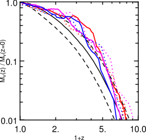
Figure 2: Mass assembly histories of LG halos in the CLUES simulation as a function of redshift. The solid black line shows the median MAH for all halos in the CLUES simulations within the mass range $5.0\times 10^{11}{{h^{-1}{\rm{M_{\odot}}}}}<M_{h}<5.0\times 10^{12}{{h^{-1}{\rm{M_{\odot}}}}}$, the dashed lines show the first and third quartiles. Also plotted as colour lines are the MAHs for the MW (dotted) and M31 halos (continuous) in the three constrained simulations. The assembly history for the LG halos is systematically located over the median values as sign of early assembly with respect to all halos in the same mass range.

3 Selection of Local Groups and Control Samples

Table 2: Names and description of the four samples used to quantify the formation history of the LG halos. The three first samples are constructed both from the CLUES and Bolshoi simulations. By definition the LG sample can only be constructed from the CLUES simulations. The size refers to the total number of objects in the corresponding volume (individual halos or pairs).

Name	Description	Size (CLUES)	Size (Bolshoi)
Individuals	All the distinct halos in the mass range $5.0\times 10^{11}$$h^{-1}{\rm{M_{\odot}}}$- $5.0\times 10^{12}$$h^{-1}{\rm{M_{\odot}}}$	4278	88756
Pairs	All the pairs of halos constructed from the Individuals sample.	1101	21877
Isolated Pairs	Subset from the Pairs sample following some isolation criteria (see §3)	85	1785
LG	The three pairs of LG halos from the constrained simulations.	3	—

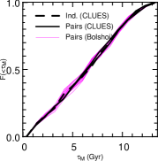
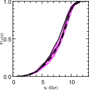
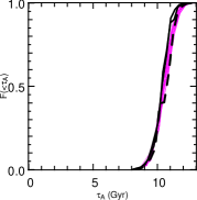
Figure 3: Fraction of halos with merger histories described by a MAHs with $\tau_{M}$, $\tau_{F}$ and $\tau_{A}$ larger than a given value. The lines represent different samples. The sample of Individuals (dashed) and Pairs (thick continuous lines) from the CLUES simulations and the Pairs extracted from eight sub-volumes in the Bolshoi simulation (thin continuous lines).

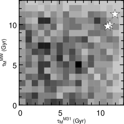
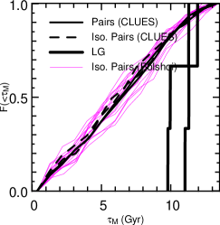
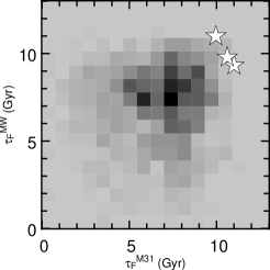
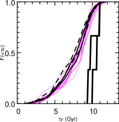
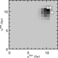
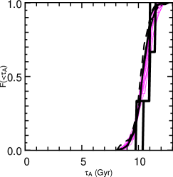
Figure 4: Left column. Joint distributions of three different times (last major merger, formation and assembly) describing the mass aggregation histories. Each point in the plane represents a pair MW-M31 with histories described by the time values at that point. Levels in shading coding indicate the number of halo pairs in the Bolshoi simulations in that parameter range. Dark regions represent a high number of pairs. An absolute scaling for this shading can be obtained from the plots presented in the Right Column. The stars mark the location of the three LG pairs, each one coming from one of the constrained simulations. Right column Integrated probability of these three different MAH times. The continuous black lines represent the results for the Pairs sample in the CLUES simulations. The Isolated Pairs sample from CLUES is represented by the thick dashed lines. The results from the Isolated Pairs samples in eight sub-volumes of the Bolshoi simulation are represented by the thin continuous grey lines. The thick continuous lines represent the results for the LG sample. The distributions from the Pairs and Isolated Pairs control samples are basically indistinguishable. In other words, detailed selection criteria for halo pairs, based on isolation only, do not narrow down significantly the range of dark matter halo assembly properties.

Four different samples of halos are constructed here, in a nested hierarchy in which the first sample contains the second which contains the third. The fourth sample is the one that includes the 3 LGs. These are to be used to study how the various criteria employed in constructing the samples affect the MAH of its members. The first three samples are constructed also from the Bolshoi simulation, and are used to look for possible biases in the constrained simulations.

The first sample we define consists of all halos in the mass range $5\times 10^{11}$$h^{-1}{\rm{M_{\odot}}}$$<M_{h}<$$5\times 10^{12}$ $h^{-1}{\rm{M_{\odot}}}$(Watkins et al., 2010). We refer to this set as the Individuals halo sample.

The second is a sample of halo pairs. Two halos, $H_{A}$ and $H_{B}$, from the Individuals sample are considered a pair if and only if halo $H_{B}$ is the closest halo to $H_{A}$ and vice-versa. Furthermore, with respect to each halo in the pair there cannot be any halo more massive than $5.0\times 10^{12}$$h^{-1}{\rm{M_{\odot}}}$closer than its companion (Karachentsev et al., 2004). We do not apply any further dynamical restrictions. For instance an element in this sample may be a pair of halos that are infalling into a cluster and are coincidentally close to each other. We refer to this set as the Pairs sample.

The third is a sample of isolated pairs. We construct it by imposing additional conditions on each member of the previous sample. These conditions are defined to obtain a LG-like halo pair according to a series of requirements that follow the lines of Governato et al. (1997), Macciò et al. (2005) Martinez-Vaquero et al. (2007). We will refer to this sample as the Isolated Pairs sample. The conditions are the following: z

1. The distance between the center of the halos is smaller than $0.7$ $h^{-1}$Mpc (Ribas et al., 2005).

2. The relative radial velocity of the two halos is negative.

3. There must not be objects more massive than either of the LG halos within a radius of $2$$h^{-1}$Mpc from each object (Tikhonov & Klypin, 2009).

4. There must not be a halo of mass $>5.0\times 10^{13}$$h^{-1}{\rm{M_{\odot}}}$within a radius of $5$$h^{-1}$Mpc with respect to each halo center (Karachentsev et al., 2004).

The final fourth sample contains the three objects that fulfil the criteria of third sample, and are located at about $10{{h^{-1}{\rm Mpc}}}$ ’south’ of the Virgo cluster in the Supergalactic Plane. This sample is referred to as LG.

We build these three samples both from the CLUES and Bolshoi simulations. A short summary description of each sample is contained in Table 2.

4 Results

The backbone of our analysis is the study of the MAH of halos in the mass range $\big{(}5.0\times 10^{11}\ -\ 5.0\times 10^{12}\big{)}$$h^{-1}{\rm{M_{\odot}}}$. Our results must be described in the 6 dimensional parameter space, spanned by the three characteristic times of the two halos, dubbed as MW and M31. The distribution of $\tau_{M}$, $\tau_{F}$ and $\tau_{A}$ of the three different samples is studied in §4.1 and the possible dependence of these distributions on the ambient density around the LGs and the mass ratio of the MW and M31 members of the LGs in §4.2.

4.1 Mass accretion history of the different samples

Figure 3 presents distribution of $\tau_{M}$, $\tau_{F}$ and $\tau_{A}$ for the Individuals and Pairs samples of both the CLUES and Bolshoi simulations. The distribution with respect to the MW and M31 are virtually indistinguishable, and the curves present both halos. We calibrate the effect of cosmic variance with the $(100{{h^{-1}{\rm Mpc}}})^{3}$ volumes extracted from the Bolshoi simulation. The results are overplotted as thin magenta lines. The distribution of $\tau_{M}$ and $\tau_{F}$ are well within the scatter of the sub-volumes, while the $\tau_{A}$ is somewhat out of the range.

We conclude that with respect to the MAH, the constrained simulations are essentially unbiased with respect to the unconstrained one. The interesting fact that emerges here is the halos in the Individuals and Pairs sample share the same MAH, as expressed by the three times described here.

Figure 4 presents the main results of the paper. It shows the distribution of the three times for the different sample of pairs of halos. The left column is made of three grey scale maps describing the number of objects in the Pairs sample in the subspace of $\big{(}\tau{{}_{X}^{M31}},\tau{{}_{X}^{MW}}\big{)}$, where $X=M,F,A$. The shades represent the number of pairs around a given region of parameter space calculated from the Pairs samples in the Bolshoi simulation. The three different LG pairs are overplotted as stars.

The right hand side column of Figure 4 shows the integrated relative distribution of the halos in the three different times of the Pairs, Isolated Pairs and LGs samples. For the LGs this is further separated for the MW and M31 halos. The distribution of the Isolated Pairs of the Bolshoi sub-volume is presented as well.

Two important comments can be made based on Figure 4. First, we see that the times in the LGs sample are confined to a narrow range compared to the broad Pairs sample. The merger, formation and assembly times in this sample are confined within the range $9.5-12$ Gyr. Second, from the integrated distribution, we infer that the Pairs and Isolated Pairs samples are virtually indistinguishable. This implies that the commonly used isolation criteria (Governato et al., 1997; Macciò et al., 2005; Martinez-Vaquero et al., 2007) do not automatically produce the narrow parameter space occupied by the LG pairs.

4.2 The influence of the Local Matter Density and the Mass Ratio

The Pairs and Isolated Pairs samples are selected based on isolation and dynamics. The similarity of the distribution of the different MAH times of the the different samples motivates us to look for the possible dependence of these distributions on some other characteristics of the three LGs. In particular, the three LGs are found to share the two following properties: the mass ratio between the two halos and the matter over-density in a sphere of $5$$h^{-1}$Mpc radius , noted as $\delta_{5}$. The values for the halo masses in the pairs and the local over-densities are listed in Table 1 together with the assembly, formation and last major merger times. A series of sub-samples of the halos sample are constructed by requiring that the masses and mass ratios between the pairs are bounded by the LG limits or the values $\delta_{5}$. These sub-sampling do not bias the LG-like objects towards the region of parameter space defined by the LG sample.

5 Discussion

Three basic facts emerge from the results presented in the previous section : a) the three LGs share a common formation history, b) this formation history is quiet out to at $\approx(10-12)$Gyr and c) none of the selection rules applied here to the pairs of halos have defined a sample of objects with MAH similar to that of the three LGs. In what follows, we discuss the possible origin and the predictable consequences of these facts.

Table 3: Fraction of halos/pairs the different samples with times $\tau_{M}$, $\tau_{F}$ and $\tau_{A}$ located in the parameter space defined by the minima characteristic times of the LG halos in the constrained simulations. These minima from the LGs are defined for each $\tau_{X}$ in two different ways: 1) as the mean value minus two times the standard deviation (see Table 1) and 2) as the minimum value of all realisations. These minima times are denoted $\tau_{X}^{\prime}$ and $\tau_{X}^{\prime\prime}$ respectively and are presented in the first rows. In the following rows, the first column describes the name and origin of the sample. The three following columns indicate the fraction of the total population with a $\tau_{X}$ larger than the calculated $\tau_{X}^{\prime}$ or $\tau_{X}^{\prime\prime}$ (in parenthesis). In the case of pairs samples, we require the times for both halos to be above the threshold. The last column refers to the three different $\tau_{X}$ being simultaneously larger than the corresponding $\tau_{X}^{\prime}$ ($\tau_{X}^{\prime\prime}$).

”Two sigma” bound	$\tau_{M}^{\prime}$ [Gyr]	$\tau_{F}^{\prime}$ [Gyr]	$\tau_{A}^{\prime}$ [Gyr]
	9.3	9.0	9.6
”Minima” bound	$\tau_{M}^{\prime\prime}$ [Gyr]	$\tau_{F}^{\prime\prime}$ [Gyr]	$\tau_{A}^{\prime\prime}$ [Gyr]
	9.8	9.3	9.7
Sample	$\tau_{M}\geq\tau_{M}^{\prime}$ ($\tau_{M}^{\prime\prime}$)	$\tau_{F}\geq\tau_{F}^{\prime}$ ($\tau_{F}^{\prime\prime}$)	$\tau_{A}\geq\tau_{A}^{\prime}$ ($\tau_{A}^{\prime\prime}$)	$\tau_{M,F,A}\geq\tau_{M,F,A}^{\prime}$ ($\tau_{M,F,A}^{\prime\prime}$)
CLUES Individuals	0.24 (0.18)	0.29 (0.24)	0.85 (0.85)	0.17 (0.12)
CLUES Pairs	0.06 (0.03)	0.09 (0.06)	0.74 (0.74)	0.03 (0.01)
CLUES Isolated Pairs	0.06 (0.03)	0.08 (0.05)	0.70 (0.70)	0.05 (0.03)
Bolshoi Individuals	0.23 (0.19)	0.23 (0.23)	0.87 (0.87)	0.17 (0.12)
Bolshoi Pairs	0.05 (0.04)	0.10 (0.05)	0.76 (0.76)	0.03 (0.02)
Bolshoi Isolated Pairs	0.05 (0.03)	0.10 (0.06)	0.73 (0.73)	0.03 (0.01)

5.1 On the Common Formation History

Naively, one might hypothesise that the fact that all three CLUES LGs have a common MAH, as defined here, is consistent with being drawn at random from the sample of pairs, i.e. the range of properties spanned by three random halo pairs can be naturally expected to be narrow. This is the null hypothesis we test now.

What is the probability that 3 randomly selected pairs have MAHs within the range of properties found for the LG? We compute this probability based on the fraction of halos in the pair samples that share the LG formation properties.

We define first the minimal subspace that contains the 3 simulated LGs by providing lower bounds on the different times describing the MAHs. Table 3 lists the minimal last major merger, formation and assembly look-back times, where two options are taken to estimate the minima. The first defines the ”two sigma” bound, namely the average value minus twice the standard deviation of each time of the 6 halos of the 3 LGs, the second takes the minimum value for each time.

The table provides the fraction of halos in the Individuals sample satisfying each one of the conditions $\tau_{X}\geq\tau_{X}^{\rm bound}$ independently and all of them simultaneously, where $X=M$, $F$ and $A$ and the subscript ${bound}$ denotes the minimal bound of such time. We find that the fraction of Individuals in the quiet MAH subspace is $f_{i}=0.17(0.12)$ both in CLUES and Bolshoi for the first (second) minima option. If we consider now the halos either in the Pairs or Isolated Pairs samples, only a fraction of $f_{p}=0.03(0.01)$ pairs are composed of halos that are both within the LG parameter space. To a good approximation, the pair fraction can be calculated as the individual fraction squared, $f_{p}\approx f_{i}\times f_{i}$. This is the expected result under the assumption that the assembly of the MW and M31 are independent.

The probability of randomly selecting three random halo pairs and having them within the range of parameters defined by the LG can be calculated as $p_{LG}=f_{p}^{3}\approx 2.7\times 10^{-5}(1.0\times 10^{-6})$. This small probability is a consequence of having found 3 halo pairs within a set of properties shared by $0.17(0.12)$ of the total population of halos. If we consider pairs with a range of desired properties within shared by, say, $0.68$ of the halos in the total population (the fraction within one standard deviation around the mean), the probability of finding three pairs inside that range would be $p_{1-\sigma}(0.68\times 0.68)^{3}\approx 0.1$.

Comparing the results of the probabilities $p_{LG}$ and $p_{1-\sigma}$, the null hypothesis can be safely rejected. It is highly unlikely that the three randomly selected pairs show a narrow range of properties as in the case of the LG sample.

Both the ab-initio and post-factum constraints imposed on the LG yield a LG sample with very similar MAHs. In the CLUES simulations only the large and mid-scales are effectively constrained by the data leaving the galactic and smaller scales effectively random. It follows that the MAH of objects similar to the LG is strongly affected by their environment. To what extent this is valid for DM halos in general remains an open question.

5.2 On the Quietness of the Formation History

We established in the previous sections that the MAHs are quiet out to $\approx(10-12)$Gyr, and that none of the selection rules applied here to the pairs of halos have defined a sample of objects with MAH similar to that of the three LGs.

The last point is consistent with the results previous studies that have approached the same question of estimating a possible bias of the LG with respect to a general halo population (de Rossi et al., 2009; Boylan-Kolchin et al., 2010). These studies apply isolation criteria on scales of $1$$h^{-1}$Mpc over halos in the mass range we study here, and find as well that no significant bias is introduced in the isolated halo population with respect to the parent halo population.

The parameter subspace defined by the three LG cannot by explained either in terms of the isolation criteria listed at the end of §3 or by adding constraints on the values of the local over-density on $5$$h^{-1}$Mpc scales. The properties of the dynamical environment, common to all the CLUES simulations and provide the quiet formation history for a LG, remain to be found. Ideally, that result should be expressed in a suitable form to search for LG pairs in an unconstrained simulation.

Is the observed Local Group biased in the same manner? We cannot provide the answer to that question with the simulations we present in this paper. Nonetheless, the theoretical predictions we show here for the dark matter assembly in the LG seem to be in agreement with the disk dominated morphology of MW and M31.

5.3 The Connection with the Observed Local Group

The most distinct feature of the MW and M31 is that both galaxies have a disk dominated morphology. It is often mentioned that abundant mergers, which are presumed to destroy the disk and be source of morphological change, are expected on all mass scales in the hierarchical picture of galaxy formation of $\Lambda$CDM  generating a possible contradiction with the abundance of disk galaxies in the local Universe and, in particular, with the fact that the MW and M31 are disk galaxies (Toth & Ostriker, 1992; Quinn et al., 1993; Kazantzidis et al., 2008).

Our results provide new theoretical evidence that the MW and M31 could be expected to be disk dominated galaxies in $\Lambda$CDM. From the results presented here, we have found that the last merger started on average $11$ Gyr ago. At these redshifts the mass of the MW host halo is $1-4\times 10^{11}$$h^{-1}{\rm{M_{\odot}}}$, its virial velocity is $\approx 200$ km/s and its virial radius $\approx 0.1$ $h^{-1}$Mpc . Using these quantities and Eq. 2 we estimate the final infall time for the satellite to be $\approx 3.5$ Gyr, reaching the center $\approx 7.5$ Gyr ago. This quiet history should favour the survival of a disk formed in the halo (Guedes et al., 2011). Although, detailed estimations on these matters might have to include the inflow of gas into the disk (Scannapieco et al., 2009).

A distinct and well characterised feature of the MW is the thick disk. This disk component of the MW has been known for more than 25 years (Gilmore & Reid, 1983). The thick disk contains a population of stars with different kinematics, spatial distribution, ages and chemical enrichment compared to the thin galactic disk. Although M31 seems to have a similar component (Collins et al., 2011), the observational and theoretical work on the MW’s thick disk has a long history, and its origin can therefore be discussed in greater detail. One of the possible formation scenarios for the MW thick disk is an in-situ formation during/after a gas rich merger (Sales et al., 2009). The analysis of the orbital eccentricity of stars based on RAVE and SDSS data supports the gas-rich merger mechanism (Dierickx et al., 2010; Wilson et al., 2011). In our results the last merger reaches the center $\approx 7.5$ Gyr ago, close to the look-back time of $8$Gyr as required by the in-situ formation scenario.

6 Conclusions

We use constrained simulations of the local Universe to study the dark matter mass aggregation history (MAH) of the Local Group (LG). Two basic questions motivate this study: 1. To what extent the simulated LGs can account for the observed structure of the MW and M31 galaxies? Namely, if the disk dominated morphology implies that the MW and M31 halos had a quiet MAH over the last $\approx 11$Gyrs, can simulations recover this recent quiet history? 2. Does this quiet MAH arise from the intrinsic properties of the DM halos, or is it induced by environment within which the LG is embedded? Is the implied MAH of the LG triggered by the large and meso-scales, or is it induced by the small, i.e. galactic and sub-galactic, scales?

The methodology adopted here is to use constrained simulations of the local Universe, designed to reproduce the large and meso-scales of the LG environment, and search for halos that resemble the actual LG. The identification of a pair of halos as a LG-like object is based on a set of isolation and dynamical criteria, all formulated by their redshift zero structure, in complete ignorance of their formation history. A LG-like object that is found close to the actual position of the observed LG with respect to the large scale structure environment is defined here as a LG. By construction a constrained simulation can have only one LG or none at all. Indeed, out of a suit of 200 constrained simulations only 3 harbour a LG. Controlled samples of individual halos and pairs have been constructed as reference samples. The analysis has been extended to the unconstrained Bolshoi simulation that is used here for an unbiased reference (Klypin et al., 2010).

The construction of the identification of the 3 LGs is done independently of the MAH of the halos. Yet, the MW’s and M31’s halos of the 3 LGs all have a common quiet MAH, defined as having the last major merger, formation and assembly look-back time extending over $\approx(10\ -12)$ Gyr. This quiet formation history of the simulated LGs can help to explain the disk dominated morphology of the MW and M31, adding evidence to the internal instability origin of the spheroidal component of the MW (Shen et al., 2010). Based on measurements of the eccentricity of orbits in the MW, it has been recently claimed (Sales et al., 2009; Dierickx et al., 2010; Wilson et al., 2011), that a rich merger taking place 10.5 to 8 Gyr ago is a favoured mechanism explain the thick disk in the MW Brook et al. (2004). Our finding of a quiet MAH of the LG provides a suitable platform for such a process to take place.

The LG halos are assumed here to be selected from FOF halos in the mass range $5\times 10^{11}{{h^{-1}{\rm{M_{\odot}}}}}<M_{h}<5\times 10^{12}{{h^{-1}{\rm{M_{\odot}}}}}$ at $z=0$. Between $12\%$ and $17\%$ of these halos are found to have a quiet MAH, depending on the detailed definition of the quiet parameter space. From this point of view the MW and M31 halos are not rare. However, how likely is a pair of halos to have such a quiet history, shared by both halos? Making the naive null assumption that the MAH of a halo is an intrinsic property of a halo independent of its environment then the fraction of pairs should be the product of the fractions for a single halo. Indeed, the Pairs sample drawn out of the Bolshoi simulation confirms this assertion, finding that between $1\%$ to $3\%$ of the pairs have as quiet an MAH as the LG systems do. The probability of having selecting 3 pairs randomly and finding them with a quiet MAH is on the order of $\sim 10^{-5}$.

Next, we look for what dynamical or environmental property determines rethe MAH of a LG-like object. We find here that the mere pairing of the MW-like halos does not affect the MAH fiducial times. Imposing the isolation and dynamical constraints that define the Isolated Pairs sample does not affect it either. This leaves us with an open question as to what determines the MAH of halo pairs similar to the LG. The one hint that we have is that all of the three LGs reside in the same large and meso-scale environment. We speculate that the cosmic web plays a major role in shaping the MAH of LG-like objects, although it is not yet clear what mechanism is responsible. A larger sample of constrained LGs is needed to confirm and further explore the reasons behind this result.

References

- Boylan-Kolchin et al. (2008) Boylan-Kolchin M., Ma C., Quataert E., 2008, MNRAS, 383, 93
- Boylan-Kolchin et al. (2010) Boylan-Kolchin M., Springel V., White S. D. M., Jenkins A., 2010, MNRAS, 406, 896
- Brook et al. (2004) Brook C. B., Kawata D., Gibson B. K., Freeman K. C., 2004, ApJ, 612, 894
- Collins et al. (2011) Collins M. L. M., Chapman S. C., Ibata R. A., Irwin M. J., Rich R. M., Ferguson A. M. N., Lewis G. F., Tanvir N., Koch A., 2011, MNRAS, pp 248–+
- de Rossi et al. (2009) de Rossi M. E., Tissera P. B., De Lucia G., Kauffmann G., 2009, MNRAS, 395, 210
- Dierickx et al. (2010) Dierickx M., Klement R., Rix H., Liu C., 2010, ApJL, 725, L186
- Gilmore & Reid (1983) Gilmore G., Reid N., 1983, MNRAS, 202, 1025
- Governato et al. (1997) Governato F., Moore B., Cen R., Stadel J., Lake G., Quinn T., 1997, New Astron., 2, 91
- Guedes et al. (2011) Guedes J., Callegari S., Madau P., Mayer L., 2011, ArXiv e-prints
- Hoffman & Ribak (1991) Hoffman Y., Ribak E., 1991, ApJL, 380, L5
- Hopkins et al. (2010) Hopkins P. F., Bundy K., Croton D., Hernquist L., Keres D., Khochfar S., Stewart K., Wetzel A., Younger J. D., 2010, ApJ, 715, 202
- Hopkins et al. (2010) Hopkins P. F., Croton D., Bundy K., Khochfar S., van den Bosch F., Somerville R. S., Wetzel A., Keres D., Hernquist L., Stewart K., Younger J. D., Genel S., Ma C., 2010, ApJ, 724, 915
- Karachentsev et al. (2004) Karachentsev I. D., Karachentseva V. E., Huchtmeier W. K., Makarov D. I., 2004, AJ, 127, 2031
- Kazantzidis et al. (2008) Kazantzidis S., Bullock J. S., Zentner A. R., Kravtsov A. V., Moustakas L. A., 2008, ApJ, 688, 254
- Klypin et al. (1999) Klypin A., Kravtsov A. V., Valenzuela O., Prada F., 1999, ApJ, 522, 82
- Klypin et al. (2010) Klypin A., Trujillo-Gomez S., Primack J., 2010, ArXiv e-prints
- Komatsu et al. (2009) Komatsu E., Dunkley J., Nolta M. R., Bennett C. L., Gold B., Hinshaw G., Jarosik N., Larson D., Limon M., Page L., Spergel D. N., Halpern M., Hill R. S., Kogut A., Meyer S. S., Tucker G. S., Weiland J. L., Wollack E., Wright E. L., 2009, ApJS, 180, 330
- Li et al. (2008) Li Y., Mo H. J., Gao L., 2008, MNRAS, 389, 1419
- Macciò et al. (2005) Macciò A. V., Governato F., Horellou C., 2005, MNRAS, 359, 941
- Martinez-Vaquero et al. (2007) Martinez-Vaquero L. A., Yepes G., Hoffman Y., 2007, MNRAS, 378, 1601
- McConnachie et al. (2009) McConnachie A. W., Irwin M. J., Ibata R. A., Dubinski J., Widrow L. M., Martin N. F., Côté P., Dotter A. L., Navarro J. F., Ferguson A. M. N., Puzia T. H., Lewis G. F., Babul A., Barmby P., Bienaymé O., Chapman S. C., Cockcroft R., 2009, Nature, 461, 66
- Metz et al. (2009) Metz M., Kroupa P., Jerjen H., 2009, MNRAS, 394, 2223
- Moore et al. (1999) Moore B., Ghigna S., Governato F., Lake G., Quinn T., Stadel J., Tozzi P., 1999, ApJL, 524, L19
- More et al. (2011) More S., Kravtsov A., Dalal N., Gottlöber S., 2011, ArXiv e-prints
- Neistein et al. (2006) Neistein E., van den Bosch F. C., Dekel A., 2006, MNRAS, 372, 933
- Quinn et al. (1993) Quinn P. J., Hernquist L., Fullagar D. P., 1993, ApJ, 403, 74
- Reiprich & Böhringer (2002) Reiprich T. H., Böhringer H., 2002, ApJ, 567, 716
- Ribas et al. (2005) Ribas I., Jordi C., Vilardell F., Fitzpatrick E. L., Hilditch R. W., Guinan E. F., 2005, ApJL, 635, L37
- Sales et al. (2009) Sales L. V., Helmi A., Abadi M. G., Brook C. B., Gómez F. A., Roškar R., Debattista V. P., House E., Steinmetz M., Villalobos Á., 2009, MNRAS, 400, L61
- Scannapieco et al. (2009) Scannapieco C., White S. D. M., Springel V., Tissera P. B., 2009, MNRAS, 396, 696
- Shen et al. (2010) Shen J., Rich R. M., Kormendy J., Howard C. D., De Propris R., Kunder A., 2010, ApJL, 720, L72
- Springel (2005) Springel V., 2005, MNRAS, 364, 1105
- Tikhonov & Klypin (2009) Tikhonov A. V., Klypin A., 2009, MNRAS, 395, 1915
- Tonry et al. (2001) Tonry J. L., Dressler A., Blakeslee J. P., Ajhar E. A., Fletcher A. B., Luppino G. A., Metzger M. R., Moore C. B., 2001, ApJ, 546, 681
- Toth & Ostriker (1992) Toth G., Ostriker J. P., 1992, ApJ, 389, 5
- Watkins et al. (2010) Watkins L. L., Evans N. W., An J. H., 2010, MNRAS, 406, 264
- Willick et al. (1997) Willick J. A., Courteau S., Faber S. M., Burstein D., Dekel A., Strauss M. A., 1997, ApJS, 109, 333
- Wilson et al. (2011) Wilson M. L., Helmi A., Morrison H. L., Breddels M. A., Bienaymé O., Binney J., Bland-Hawthorn J., 2011, MNRAS, pp 260–+