Scattering theory of topological insulators and superconductors

Abstract

The topological invariant of a topological insulator (or superconductor) is given by the number of symmetry-protected edge states present at the Fermi level. Despite this fact, established expressions for the topological invariant require knowledge of all states below the Fermi energy. Here, we propose a way to calculate the topological invariant employing solely its scattering matrix at the Fermi level without knowledge of the full spectrum. Since the approach based on scattering matrices requires much less information than the Hamiltonian-based approaches (surface versus bulk), it is numerically more efficient. In particular, is better-suited for studying disordered systems. Moreover, it directly connects the topological invariant to transport properties potentially providing a new way to probe topological phases.

I Introduction

Given a Hamiltonian $H(\bm{k})$ of a band insulator or a superconductor and its symmetries as a function of the momentum $\bm{k}$ in $d$-spatial dimensions, a topological invariant $\mathcal{Q}(H)$ can be defined. It counts the number of surface states insensitive to disorder which are present at an interface between the system and the vacuum. In each spatial dimension exactly 5 out of 10 Altland-Zirnbauer symmetry classes (distinguished by time-reversal symmetry $\mathcal{T}$, particle-hole symmetry $\mathcal{P}$, and chiral/sub-lattice symmetry $\mathcal{C}$)Altland and Zirnbauer (1997) allow for a nontrivial topological invariant.Kitaev (2009); Schnyder et al. (2009)

The evaluation of the topological invariant conventionally involves an integral over a $d$-dimensional Brillouin zone of some function of the Hamiltonian. Recently, various approximations to the topological invariant have been developed which require only the knowledge of eigenvalues and eigenvectors of the Hamiltonian at one point in momentum space (rather than in the entire Brillouin zone).Loring and Hastings (2010); Ringel and Kraus (2011); Hastings and Loring (2011)

Despite the fact that these approximations are more efficient, we argue that they do not use one important property of a topological invariant. By definition, the topological invariant describes the properties of the system at the Fermi level, namely the number of edge states. This observation suggests that it should be possible to calculate the topological invariant without knowing the full spectrum of the Hamiltonian, but rather calculating only properties of the system at its Fermi energy. For one-dimensional (1D) systems, this was demonstrated in Ref. Fulga et al., 2011. Here, we show that for any dimensionality the topological invariant can be obtained from the scattering matrix of the system at the Fermi level.

Our results offer two benefits. Firstly, since the scattering matrix contains less degrees of freedom than the Hamiltonian, the computation of the topological invariant is much more efficient. Secondly, the scattering matrix relates the topological invariant to transport properties, suggesting ways to probe the topological phase by electrical or thermal conduction measurements.Akhmerov et al. (2011); Wimmer et al. (2011)

The approach is based on dimensional reduction: We relate the scattering matrix in $d$ dimensions to a Hamiltonian in $d-1$ dimensions. Our scheme of dimensional reduction does not preserve the symmetry, unlike the field theory based scheme of Ref. Qi et al., 2008. Instead our dimensional reduction preserves the topological invariant, similarly to the dimensional reduction of clean Dirac-like Hamiltonians of Ref. Ryu et al., 2010a.

In the remainder of the introduction we first illustrate our approach by revisiting the familiar example of the integer quantum Hall effect. Subsequently, we present a brief outline of the paper.

I.1 Dimensional reduction in the quantum Hall effect

A 2D system exhibiting the integer quantum Hall effect is a topological insulator in the symmetry class A (all symmetries broken). It is characterized by a quantized transverse conductance $\sigma_{xy}=ng_{0}$ with $n\in\mathbb{Z}$ and $g_{0}=e^{2}/h$. The quantum number $n$ is a topological invariant (the so-called Chern number) of the Hamiltonian.Thouless et al. (1982) It equals the number of protected chiral edge states at the Fermi level, each of which contributes $e^{2}/h$ to the transverse conductance.Halperin (1982); Büttiker (1988)

Charge pumping provides an alternative way to relate the topological invariant to a quantized transport property: inserting a flux quantum inside a quantum Hall sample rolled-up to a cylinder adiabatically pumps $n$ electrons across the sample.Laughlin (1981) There exists a scattering matrix formulation of charge pumping,Büttiker et al. (1994); Brouwer (1998) which allows to express pumped charge per cycle (in units of $e$),

$$\mathcal{Q}=\frac{1}{2\pi i}\int_{0}^{2\pi}\!\!d\varphi\,\frac{d}{d\varphi}\log\det r(\varphi),$$ (1)

through the flux dependence of the reflection block $r(\varphi)$ of the scattering matrix of one lead.Bräunlich et al. (2010) Here $\varphi$ denotes the dimensionless flux $\Phi=\hbar\varphi/e$ and the system is assumed to be insulating such that the reflection matrix $r(\varphi)$ is unitary. Equation (1) is nothing but the winding number of $\det r(\varphi)$ when $\varphi$ is varied from $0$ to $2\pi$, which is a topological invariant.

The winding number occurs in a different context in the theory of topological insulators. The topological invariant of a one-dimensional Hamiltonian $H(k)$ with chiral/sub-lattice symmetry

$$H(k)=\begin{pmatrix}0&h(k)\\ h^{\dagger}(k)&0\end{pmatrix},$$ (2)

is expressed via the winding number given byZak (1989); Ryu and Hatsugai (2002)

$$\mathcal{Q}(H)=\frac{1}{2\pi i}\int_{0}^{2\pi}\!\!dk\,\frac{d}{dk}\log\det h(k).$$ (3)

Here momentum $k$ is measured in units of $\hbar/a$, with $a$ the lattice constant. We see that upon the identification $h\equiv r$ and $k\equiv\varphi$ we are able to express the topological invariant in a 2D system without any symmetries as the topological invariant of an effective Hamiltonian in 1D with chiral symmetry. We will show that a similar dimensional reduction applies to all topological invariants in all dimensions.

I.2 Outline of the paper

As a prerequisite for the dimensional reduction, we have to open up the system to obtain a scattering matrix from a given Hamiltonian. Section II explains how this can be done. This section may be skipped on first reading. The dimensional reduction proceeds along the following lines: First we form out of a scattering matrix $S$ a reflection block $r(\bm{k})$ from one surface of the system, when all the dimensions except one are closed by twisted periodic boundary conditions. Then, the effective Hamiltonian $H_{d-1}(\bm{k})$ in one dimension lower is defined according to the simple rule

$$H_{d-1}(\bm{k})\equiv r(\bm{k}),\textrm{\quad with chiral symmetry,}$$ (4a)

$$H_{d-1}(\bm{k})\equiv\begin{pmatrix}0&r(\bm{k})\\ r^{\dagger}(\bm{k})&0\end{pmatrix},\textrm{\quad without chiral symmetry.}$$ (4b)

In Sec. III we show how to evaluate $r(\bm{k})$ given the scattering matrix $S$ of the initial system and prove that the reduced Hamiltonian $H_{d-1}$ has the same topological invariant as the original $H$, i.e. $\mathcal{Q}(H_{d-1})=\mathcal{Q}(H)$.

After the general proof we turn to the particular ways to evaluate the topological invariant in 1–3 dimensions in Sec. IV. In 1D we show that our expressions coincide with the ones derived in Ref. Fulga et al., 2011 in a different way, without using dimensional reduction. For 2D we formulate the evaluation of the topological invariant as a generalized eigenvalue problem. For 3D topological insulators in class AII the topological invariant reduces to a product of 2D invariants, while the other symmetry classes require usage of a Bott index.Hastings and Loring (2011) We also mention how weak topological invariants fit into our approach.

We consider the numerical efficiency of our method and show examples of its application in Sec. V. We also compare the finite size effects of different approximations to the topological invariant, and introduce the ‘fingerprint’ of phase transitions between different topological phases in 2D. Finally, we conclude in Sec. VI.

II Scattering matrix from a Hamiltonian

This section contains the necessary preliminaries: the definition of scattering matrix and a proof that the shape of the Fermi surface can be calculated from the scattering matrix.

While the formulas in this section are needed for the actual implementation of our method of dimensional reduction, the method itself can be understood without them. This section can thus be skipped at first reading.

Any Hamiltonian $H(\bm{k})$ of a translationally invariant system with a finite range hopping can be brought to the tight-binding form by choosing a sufficiently large unit cell

$$H(\bm{k})=H+\sum_{i=0}^{d}t_{i}e^{ik_{i}}+\sum_{i=0}^{d}t_{i}^{\dagger}e^{-ik_{i}}.$$ (5)

Here $\bm{k}$ is a $d$-dimensional vector of Bloch momenta, $H$ is the on-site Hamiltonian, and $t_{i}$ are the hoppings in positive $i$-direction. We start our consideration from opening the system and attaching $2d$ fictitious leads to it. First we attach $d$ sites to the original system without on-site Hamiltonian, and connect them with hoppings $t_{i}$ to the system. The Hamiltonian of this ‘unfolded’ system becomes

$$\tilde{H}=\begin{pmatrix}H&t^{\dagger}\\ t&0\end{pmatrix},$$ (6)

$$t=(t_{1},t_{2},\ldots t_{d})^{T}.$$ (7)

In the next step we attach the fictitious leads to the unfolded system, as illustrated in Fig. 1 for the case of two dimensions. The hopping to the leads in positive $i$-direction is chosen to be equal to $+1$, and in the negative $i$-direction to be equal to $-1$.

Figure 1: Sketch of the tight binding model used to attach leads in order to open-up the Hamiltonian $H(\bm{k})$ of (5). In 2D we introduce four leads shown as circles labeled by $1$, $\bar{1}$, $2$, and $\bar{2}$. The on-site terms (boxes) are connected by hoppings (lines). The additional trivial hoppings $1$ and $-1$ are introduced such that the lead properties drop out when twisted periodic boundary conditions are applied. For the Mahaux-Weidenmüller formula (8), the three nodes form the on-site Hamiltonian $\tilde{H}$ which is then connected via the trivial hoppings to ideal leads.

We are now ready to construct the scattering matrix of the open system by using the Mahaux-Weidenmüller formulaMahaux and Weidenmüller (1969) (see also Appendix A)

$$S=1+2\pi iW^{\dagger}(\tilde{H}-i\pi WW^{\dagger})^{-1}W.$$ (8)

The coupling $W$ between the lead and the system is equal to $w\sqrt{\rho}$, with $w$ the hopping from the lead to the system, and $\rho$ the density of states in the lead. We choose $\rho=1/w\pi$, such that

$$W=\frac{1}{\sqrt{\pi}}\begin{pmatrix}1&0&1&0&\cdots&1&0\\ 0&-1&0&0&&0&0\\ 0&0&0&-1&&0&0\\ \vdots&&&&\ddots&&\vdots\\ 0&0&0&0&\cdots&0&-1\end{pmatrix};$$ (9)

here, we have set $w=1$ for convenience. The values of hopping and the lead density of states are chosen such that in the process of rolling-up, the fictitious leads drop out.

The scattering matrix (8) relates the incoming states in the leads to the outgoing ones:

$$\begin{pmatrix}\psi_{1}\\ \psi_{\bar{1}}\\ \psi_{2}\\ \psi_{\bar{2}}\\ \vdots\\ \psi_{d}\\ \psi_{\bar{d}}\end{pmatrix}_{\text{out}}=S\begin{pmatrix}\psi_{1}\\ \psi_{\bar{1}}\\ \psi_{2}\\ \psi_{\bar{2}}\\ \vdots\\ \psi_{d}\\ \psi_{\bar{d}}\end{pmatrix}_{\text{in}}.$$ (10)

To prove that the scattering matrix contains all of the information about the Fermi level at energy $E_{F}=0$, we impose twisted periodic boundary conditions on the scattering states:

$$\begin{pmatrix}\psi_{1}\\ \psi_{\bar{1}}\\ \psi_{2}\\ \psi_{\bar{2}}\\ \vdots\\ \psi_{d}\\ \psi_{\bar{d}}\end{pmatrix}_{\text{in}}=Z(\bm{k})\begin{pmatrix}\psi_{1}\\ \psi_{\bar{1}}\\ \psi_{2}\\ \psi_{\bar{2}}\\ \vdots\\ \psi_{d}\\ \psi_{\bar{d}}\end{pmatrix}_{\text{out}},$$ (11)

with the twist matrix $Z(\bm{k})$ given by

$$Z(\bm{k})\equiv\begin{pmatrix}0&e^{ik_{1}}&0&\cdots&0\\ e^{-ik_{1}}&0&&&\vdots\\ 0&&\ddots&&0\\ \vdots&&&0&e^{ik_{d}}\\ 0&\cdots&0&e^{-ik_{d}}&0\end{pmatrix}.$$ (12)

We show that Eqs. (10) and (11) have a solution for a given $\bm{k}$ if and only if the equation $H(\bm{k})\psi=0$ has a nontrivial solution. The condition for the nontrivial solution of Eqs. (10) and (11) to exist is

$$\det[S-Z(\bm{k})]=0.$$ (13)

Performing block-wise inversion of $\tilde{H}-i\pi WW^{\dagger}$ yields

$$S=1+2iW^{\dagger}\begin{pmatrix}J&-iJt^{\dagger}\\ -itJ&i-tJt^{\dagger}\end{pmatrix}W,$$ (14)

$$J=(H_{0}-id-it^{\dagger}t)^{-1}.$$ (15)

We simplify this expression further by noting that

$$S =\gamma_{z}+2i\gamma_{z}U^{\dagger}JU, U =\begin{pmatrix}1&-it^{\dagger}\end{pmatrix}W,$$ (16)

with $\gamma_{z}$ the third Pauli matrix in the direction space. We now write

$$\det[S-Z(\bm{k})] =\det\left[1+\gamma_{z}Z(\bm{k})+2iU^{\dagger}JU\right]$$ (17)

$$=\det J\det[1+\gamma_{z}Z(\bm{k})]$$

$$\quad\times\det\left(J^{-1}+2iU[1+\gamma_{z}Z(\bm{k})]U^{\dagger}\right)$$

$$=\det J\det[1+\gamma_{z}Z(\bm{k})]\det H(\bm{k}).$$

Since both $J$ and $1+\gamma_{z}Z(\bm{k})$ are nonsingular, the last identity means that $\det[S-Z(\bm{k})]$ and $\det H(\bm{k})$ can only be zero simultaneously, which is what we set out to prove.

This proof shows that the Fermi surfaces as defined by the original Hamiltonian and the scattering matrix are identical. This is the reason why it is at all possible to determine the topological invariant using solely the scattering matrix $S$. Even though the scattering matrix only describes scattering at the Fermi level, it contains information about the complete Brillouin zone, and thus cannot be obtained from a long wavelength or low energy expansion of the Hamiltonian, but requires the complete Hamiltonian. Note however that the scattering matrix at a single energy contains less information about the system than the Hamiltonian: in order to determine the Hamiltonian from the scattering matrix, the inverse scattering problem has to be solved which requires knowledge of the scattering matrix at all the energies.

The size of the scattering matrix (8) is $2d$-times larger than the size of Hamiltonian. However, if the Hamiltonian is local on a large $d$-dimensional lattice with size $L^{d}$, the hoppings $t_{i}$ are very sparse. This allows to efficiently eliminate all of the modes except the ones that are coupled to the hoppings. The resulting scattering matrix is of size $2dL^{d-1}$, and accordingly for large systems it is a dense matrix of much smaller dimensions than the Hamiltonian.

III Dimensional reduction

The aim of this section is to provide a route to the topological classification of scattering matrices by elimination of one spatial dimensions. This approach of dimensional reduction is inspired by the transport properties of topological systems. When applied to 1D systems it reproduces the results of Ref. Fulga et al., 2011, and in quantum Hall systems it reproduces the relation between adiabatic pumping and the Chern number of Refs. Laughlin, 1981; Bräunlich et al., 2010.

We begin from substituting the first $2(d-1)$ equations from (11) into (10). This is equivalent to applying twisted periodic boundary conditions to all of the dimensions except the last one, which is left open. Then we study the reflection from the $d$-direction back onto itself. The reflection is given by

$$\psi_{d\textrm{,out}}=r(\bm{k})\psi_{d\textrm{,in}},$$ (18)

$$r(\bm{k})=D-C[A-Z_{d-1}(\bm{k})]^{-1}B,$$ (19)

with $Z_{d-1}$ given by Eq. (12) in $d-1$ dimensions. The matrices $A$, $B$, $C$, and $D$ are sub-blocks of $S$ given by

$$A =\begin{pmatrix}S_{1,1}&\cdots&S_{1,\overline{d-1}}\\ \vdots&\ddots&\vdots\\ S_{\overline{d-1},1}&\cdots&S_{\overline{d-1},\overline{d-1}}\end{pmatrix}, B= \begin{pmatrix}S_{1,d}\\ \vdots\\ S_{\overline{d-1},d}\end{pmatrix},$$

$$C =\begin{pmatrix}S_{d,1}&\cdots&S_{d,\overline{d-1}}\end{pmatrix}, D =\begin{pmatrix}S_{d,d}\end{pmatrix}.$$ (20)

To study topological properties of $r(\bm{k})$ we construct an effective Hamiltonian $H_{d-1}(\bm{k})$ which has band gap closings whenever $r(\bm{k})$ has zero eigenvalues. In classes possessing chiral symmetry one may choose a basis such that $r(\bm{k})=r^{\dagger}(\bm{k})$. If chiral symmetry is absent, there is no Hermiticity condition on $r$, so we double the degrees of freedom to construct a single Hermitian matrix out of a complex one. The effective Hamiltonian is then given by

$$H_{d-1}(\bm{k})\equiv r(\bm{k}),\textrm{\quad with chiral symmetry,}$$ (21a)

$$H_{d-1}(\bm{k})\equiv\begin{pmatrix}0&r(\bm{k})\\ r^{\dagger}(\bm{k})&0\end{pmatrix},\textrm{\quad without chiral symmetry.}$$ (21b)

It is straightforward to verify that in both cases the Hamiltonian $H_{d-1}(\bm{k})$ has band gap closings simultaneously with the appearance of vanishing eigenvalues of $r(\bm{k})$.

If $r(\bm{k})$ has chiral symmetry, $H_{d-1}(\bm{k})$ does not have it. On the other hand, if $r(\bm{k})$ has no chiral symmetry, then

$$H_{d-1}(\bm{k})=-\tau_{z}H_{d-1}(\bm{k})\tau_{z},$$ (22)

with $\tau_{z}$ the third Pauli matrix in the space of the doubled degrees of freedom. This means that in that case $H_{d-1}(\bm{k})$ acquires chiral symmetry.

The way in which the dimensional reduction changes the symmetry class is summarized in Fig. 2. The transformation of symmetries of $r(\bm{k})$ into symmetries of $H_{d-1}(\bm{k})$ is straightforward in all of the cases, except the time-reversal symmetry in symmetry classes AII and AI. There we have $r(\bm{k})=\pm r^{T}(-\bm{k})$, and hence

$$H_{d-1}(\bm{k})\equiv\begin{pmatrix}0&r(\bm{k})\\ r^{\dagger}(\bm{k})&0\end{pmatrix}=\\ \begin{pmatrix}0&\pm r(-\bm{k})^{T}\\ \pm[r^{T}(-\bm{k})]^{\dagger}&0\end{pmatrix}=\pm\tau_{x}H_{d-1}^{*}(-\bm{k})\tau_{x}.$$ (23)

The details of the symmetry properties of $r$ and $H$, as well as the relations between these symmetries are given in App. A.

Figure 2: Symmetry properties of $r(\bm{k})$ and $H(\bm{k})$ in the ten symmetry classes. Time-reversal symmetry is denoted by $\mathcal{T}$, particle-hole symmetry by $\mathcal{P}$. The signs at the top and left of the table denote either the absence ($\times$) of a corresponding symmetry, or the value of the squared symmetry operator. The entries of the table with a gray background have an additional chiral symmetry $\mathcal{C}$, which always has the form shown in the AIII entry of the table. In particular, we always chose a basis such that $r(\bm{k})=r^{\dagger}(\bm{k})$ in the chiral symmetry classes. The way symmetry classes transform under our definition of $H_{d-1}$, cf. (21), is denoted by the arrows; the double arrow implies a doubling of degrees of freedom as in Eq. (21b). Going along an arrow, the symmetry of the reflection block $r(\bf{k})$ (marked by a solid box) transforms into the symmetry of the reduced Hamiltonian (marked by a dashed box). In the chiral classes, there is an additional symmetry (not marked by a box) which can be obtained from the other by combining it with the chiral symmetry, $H(\bm{k})=-\tau_{z}H(\bm{k})\tau_{z}$ and $r(\bm{k})=r^{\dagger}(\bm{k})$, respectively.

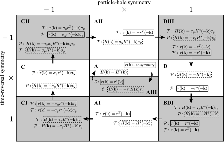
The way the symmetry class of the $d$-dimensional Hamiltonian transforms into the symmetry class of $H_{d-1}(\bm{k})$ expresses the Bott periodicity of the topological classification of symmetry classes.Kitaev (2009) Namely, symmetry classes A and AIII transform into each other, and the other 8 classes with anti-unitary symmetries are shifted by one, as shown in Table 1. This reproduces the natural succession of symmetry classes that appears in the context of symmetry breakingStone et al. (2011) (see also Appendix A). The combined effects of the change in dimensionality and in symmetry class is that the Hamiltonians $H(\bm{k})$ and $H_{d-1}(\bm{k})$ have the same topological classification.

Table 1: (Color online) Topological classification of the ten symmetry classes in different dimensions. Combinations of symmetry class and dimensionality which support non-trivial topological invariants are indicated by the type of the topological invariant ($\mathbb{Z}$ or $\mathbb{Z}_{2}$). Classes which support only trivial insulators are denoted by ‘-’. The arrows indicate the change of symmetry class upon dimensional reduction as discussed in the main text. The topmost symmetries A and AIII (which do not have any anti-unitary symmetries) transform into each other, whereas the remaining 8 classes (with anti-unitary symmetries) exchange cyclically. The dimensional reduction changes the symmetry class, but preserves the topological invariant (‘-’, $\mathbb{Z}$, or $\mathbb{Z}_{2}$).

We now turn to prove that for localized systems topological invariants $\mathcal{Q}(H)$ and $\mathcal{Q}(H_{d-1})$ are identical. This correspondence was proven in 1D in Ref. Fulga et al., 2011, so here we accomplish the proof in higher dimensions.

First of all, we observe that a topologically trivial Hamiltonian can be deformed into a bunch of completely decoupled localized orbitals without closing its gap. In a sufficiently large system, this also means that the gap of $H_{d-1}(\bm{k})$ does not close during this process. For a system of decoupled orbitals, $r(\bm{k})$ and accordingly $H_{d-1}(\bm{k})$ are momentum-independent (and hence $H_{d-1}(\bm{k})$ is topologically trivial). This means that a sufficiently large system with trivial $H(\bm{k})$ maps onto a trivial $H_{d-1}(\bm{k})$ under the scheme of dimensional reduction outlined above.

Let us now consider an interface between two systems with different bulk Hamiltonians $H$ and $H^{\prime}$, shown in Fig. 3. If the Hamiltonians $H_{d-1}$ and $H_{d-1}^{\prime}$ constructed out of reflection blocks of the two systems have different topological invariants, a topologically protected zero energy edge state in $d-1$ dimensions must appear at the interface between them. Recalling that a zero energy edge state in $d-1$ dimension corresponds to a perfectly transmitting mode of the original $d$-dimensional system, we conclude that $H$ and $H^{\prime}$ have different topological invariants.

Figure 3: A system in $d$ dimensions consisting out of two parts with different Hamiltonians $H$ and $H^{\prime}$. Reflection blocks of the scattering matrix $r$ and $r^{\prime}$ are used to define the lower dimensional Hamiltonians $H_{d-1}$ and $H_{d-1}^{\prime}$. We prove the correspondence between topological invariants in $d$ and $d-1$ dimensions using the relation between the surface state at the interface between $H$ and $H^{\prime}$ and the edge state at the interface between $H_{d-1}$ and $H_{d-1}^{\prime}$.

Conversely, if $H$ and $H^{\prime}$ have different topological invariants, there exists a transmitting mode at the interface between two parts of the system, which appears irrespective of system size and microscopic details of the interface. This means that it is not possible to construct an interface between $H_{d-1}$ and $H_{d-1}^{\prime}$ which would be completely gapped.

Finally, the edge states in $d-1$ dimension have to have the same group properties as the surface states in $d$ dimensions, leading us to the conclusion that $\mathcal{Q}(H)=\mathcal{Q}(H_{d-1})$, as we set out to prove. The topology-preserving property of our dimensional reduction procedure is the same as that of the mapping from a general $d$-dimensional Hamiltonian to a $d+1$-dimensional Hamiltonian presented in Ref. Teo and Kane, 2010.

At this point one might wonder why we apply the dimensional reduction only once. Indeed, the reduced Hamiltonian $H_{d-1}$ can be straightforwardly approximated by a tight-binding Hamiltonian on a $d-1$ dimensional lattice using a Fourier transform. This allows to repeat the procedure of dimensional reduction until we arrive at a zero dimensional Hamiltonian. We stop at the first dimensional reduction for practical purposes, since the advantage of considering only Fermi level properties is achieved already at the first step.

IV Results for one–three dimensions

IV.1 Topological invariant in 1D

We begin by verifying that we recover the 1D results of Ref. Fulga et al., 2011, where the topological invariant was related to the scattering matrix without going through the procedure of dimensional reduction. Dimensional reduction in this case brings us to a zero-dimensional Hamiltonian. The topological invariant of a zero-dimensional Hamiltonian without symmetry between positive and negative energies (symmetry classes A, AI, and AII) is given just by the number of states below the Fermi level. In class AII Kramers’ degeneracy makes this number always even. In addition, in 0D there exist two $\mathbb{Z}_{2}$ topological insulators in symmetry classes D and BDI. The topological number is in that case the ground state fermion parity, or the Pfaffian of the Hamiltonian in the basis where it is antisymmetric. To summarize,

$$\mathcal{Q}(H) =\nu(H),$$ for A, AI, and AII, (24a)

$$\mathcal{Q}(H) =\operatorname{Pf}\,iH,$$ for D and BDI, (24b)

where $\nu(A)$ denotes the number of negative eigenvalues of the Hermitian matrix $A$. Substituting $H$ from Eqs. (21) yields

$$\mathcal{Q} =\nu(r),$$ for AIII, BDI, and CII (25a)

$$\mathcal{Q} =\operatorname{Pf}\,ir,$$ for DIII, (25b)

$$\mathcal{Q} =\operatorname{Pf}\begin{pmatrix}0&ir\\ -ir^{T}&0\end{pmatrix}$$

$$=\det r,$$ for D. (25c)

We confirm that the Eqs. (25) are in agreement with Ref. Fulga et al., 2011.

IV.2 Topological invariant in 2D

Starting from 2D, the dimensional reduction brings us to a 1D Hamiltonian. In this subsection we first review the known expressions for the topological invariants of 1D Hamiltonians, and then describe how to efficiently evaluate it for the effective Hamiltonian (21). The $\mathbb{Z}$ topological insulators in 1D (classes AIII, BDI, and CII) are characterized by a winding numberZak (1989); Ryu and Hatsugai (2002)

$$H(k) \equiv\begin{pmatrix}0&h(k)\\ h^{\dagger}(k)&0\end{pmatrix},$$ (26)

$$\mathcal{Q}(H) =\frac{1}{2\pi i}\int_{0}^{2\pi}\!\!dk\frac{d}{dk}\log\det h(k),$$

$$\hskip 130.08731pt\text{for AIII, BDI, and CII}.$$ (27)

The topological invariant for the Hamiltonian in class D is given by Kitaev’s formulaKitaev (2001)

$$\mathcal{Q}(H)=\operatorname{sign}\left[\frac{\operatorname{Pf}\,H(0)}{\operatorname{Pf}\,H(\pi)}\right],\quad\text{for D}.$$ (28)

Finally, in class DIII the expression for the topological invariant was derived in Ref. Qi et al., 2010:

$$\mathcal{Q}(H) =\frac{\operatorname{Pf}[U_{\cal T}h(\pi)]}{\operatorname{Pf}[U_{\cal T}h(0)]}\exp\Biggl{[}-\tfrac{1}{2}\int_{0}^{\pi}\!\!dk\,\frac{d}{dk}\log\det h(k)\Biggr{]}$$

$$=\frac{\operatorname{Pf}[U_{\cal T}h(\pi)]}{\operatorname{Pf}[U_{\cal T}h(0)]}\frac{\sqrt{\det h(0)}}{\sqrt{\det h(\pi)}},\quad\text{for DIII,}$$ (29)

where the square root is defined through analytic continuation over the first half of the Brillouin zone, $h$ is defined by Eq. (26), and $U_{\cal T}$ is the unitary part of the time reversal operator ${\cal T}=U_{\cal T}{\cal K}$.

Substituting Eq. (21) into the expressions for topological charge we get

$$\mathcal{Q} =\frac{1}{2\pi i}\int_{0}^{2\pi}\!\!dk\frac{d}{dk}\log\det r(k),$$ for A, C, D (30a)

$$\mathcal{Q} =\frac{\operatorname{Pf}[U_{\cal T}r(\pi)]}{\operatorname{Pf}[U_{\cal T}r(0)]}\frac{\sqrt{\det r(0)}}{\sqrt{\det r(\pi)}},$$ for AII, (30b)

$$\mathcal{Q} =\operatorname{sign}\left[\frac{\operatorname{Pf}\,r(0)}{\operatorname{Pf}\,r(\pi)}\right],$$ for DIII. (30c)

In order to efficiently evaluate the integral given in Eq. (27), and the analytic continuation in Eq. (30b) using Eq. (19), we define a new variable $z=e^{ik}$. Then we perform an analytic continuation of $\det\,r(z)$ to the complex plane from the unit circle $|z|=1$. To find zeros and poles of $\det\,r(z)$ we use

$$\det r(z)=\det\begin{pmatrix}A-Z_{1}(k)&B\\ C&D\end{pmatrix}\bigg{/}\det\left[A-Z_{1}(k)\right],$$ (31)

where

$$Z_{1}(k)=\begin{pmatrix}0&e^{ik}\\ e^{-ik}&0\end{pmatrix}=\begin{pmatrix}0&z\\ z^{-1}&0\end{pmatrix};$$

Equation (31) follows from Eq. (19) and the determinant identity

$$\det(D-CM^{-1}B)=\det\begin{pmatrix}M&B\\ C&D\end{pmatrix}\bigg{/}\det M.$$ (32)

Since both the numerator and the denominator of Eq. (31) are finite at any finite value of $z$, the roots of the numerator $z_{n}$ are the zeros of $\det r(z)$, and the roots of the denominator $w_{n}$ are the poles. In App. B we show that due to unitarity of the scattering matrix, the poles of $\det r(z)$ never cross the unit circle. By multiplying the second column of the numerator of Eq. (31) by $z$ we bring the problem of finding roots $z_{n}$ of this numerator to the generalized eigenvalue problem,

$$\begin{pmatrix}S_{1,1}&-1&S_{1,2}\\ S_{\bar{1},1}&0&S_{\bar{1},2}\\ S_{2,1}&0&S_{2,2}\end{pmatrix}\psi_{n}=z_{n}\begin{pmatrix}0&-S_{1,\bar{1}}&0\\ 1&-S_{\bar{1},\bar{1}}&0\\ 0&-S_{2,\bar{1}}&0\end{pmatrix}\psi_{n},$$ (33)

which can be efficiently evaluated. The roots $w_{n}$ of the denominator can also be found by solving the generalized eigenvalue problem,

$$\begin{pmatrix}S_{1,1}&-1\\ S_{\bar{1},1}&0\end{pmatrix}\psi_{n}=w_{n}\begin{pmatrix}0&-S_{1,\bar{1}}\\ 1&-S_{\bar{1},\bar{1}}\end{pmatrix}\psi_{n}.$$ (34)

Since the poles of $\det r(z)$ never cross the unit circle, in classes A, C, and D the topological invariant is given by

$$\mathcal{Q}=\#\{z_{n}:|z_{n}|<1\}-N_{1},\quad\text{for A, C, and D},$$ (35)

i.e., the number of $z_{n}$’s inside the unit circle minus the number of modes $N_{1}$ in the direction 1. In class AII (quantum spin Hall insulator) the topological invariant is given by

$$\mathcal{Q}=\frac{\prod_{n}\sqrt{i\frac{1+z_{n}}{1-z_{n}}}}{\prod_{n}\sqrt{(-i)\frac{1+w_{n}}{1-w_{n}}}}\times\frac{\operatorname{Pf}\,U_{\cal T}r(\pi)}{\operatorname{Pf}\,U_{\cal T}r(0)}\quad\text{for AII},$$ (36)

with the branch cut of the square root along the negative real axis. Note that the linear fractional transformation $z\mapsto i(1+z)/(1-z)$ maps the upper half of the unit circle onto the negative real axis. In symmetry class DIII the evaluation of the topological invariant is most straightforward, and yields

$$\mathcal{Q}=\operatorname{sign}\left[\frac{\operatorname{Pf}\,r(0)}{\operatorname{Pf}\,r(\pi)}\right]\quad\text{for DIII}.$$ (37)

The physical meaning of the topological invariant in class A is quantized pumping of charge as a response to magnetic flux. In the quantum spin Hall insulator in class AII the invariant can be interpreted either as time-reversal polarization pumpingFu and Kane (2006), or as pumping of spin which is quantized along an unknown axis.Meidan et al. (2011a, b) In the superconducting classes C, D, and DIII it is an analogous thermal or gravitational response.Ryu et al. (2012); Wang et al. (2011)

IV.3 Topological invariant in 3D

Turning now to 3D, we need to consider topological invariants of 2D Hamiltonians. The symmetry class with the simplest expression for the topological invariant in terms of the scattering matrix in 3D is AII. The 2D topological invariant of a system in class DIII (into which AII transforms upon dimensional reduction) is a productQi et al. (2010) of the topological invariants (IV.2) of 1D Hamiltonians obtained by setting one of the momenta to $0$ or $\pi$,

$$\mathcal{Q}[H(k_{1},k_{2})]=\mathcal{Q}[H(k_{1},0)]\mathcal{Q}[H(k_{1},\pi)],$$ (38)

with $\mathcal{Q}[H(k_{1})]$ given by Eq. (IV.2). Substituting Eq. (21) into this expression we obtain

$$\mathcal{Q}=\frac{\operatorname{Pf}[U_{\cal T}r(\pi,0)]}{\operatorname{Pf}[U_{\cal T}r(0,0)]}\frac{\sqrt{\det r(0,0)}}{\sqrt{\det r(\pi,0)}}\times\\ \frac{\operatorname{Pf}[U_{\cal T}r(\pi,\pi)]}{\operatorname{Pf}[U_{\cal T}r(0,\pi)]}\frac{\sqrt{\det r(0,\pi)}}{\sqrt{\det r(\pi,\pi)}}\textrm{,\quad for AII.}$$ (39)

Direct evaluation of the Hamiltonian topological invariant in 2D in classes with nontrivial Chern number (A, C, D), and in class AII is hard because of the need to fix the gauge throughout the Brillouin zoneThouless et al. (1982); Fu and Kane (2006). It is usually more efficient to use a method which relies on the real space structure of $H$ evaluated in a single point in momentum space.Loring and Hastings (2010); Ringel and Kraus (2011); Prodan (2011a); Loring and S rensen (2011) These methods using the Bott index or a similar expression for the topological invariant require the so-called band-projected position operators: $x_{P}=P\exp(2\pi ix)P$ and $y_{P}=P\exp(2\pi iy)P$. Here $P$ is the projector on the states of the Hamiltonian with negative energies, and $x$ and $y$ are the coordinate operators in the unit cell of the system. In order to evaluate these operators in our case we note that the eigenvalues of the effective Hamiltonian in the symmetry classes of interest approach $\pm 1$ when the original system becomes localized. In that case $P=(1-r)/2$ [with $r\equiv r(0,0)$], and we can avoid the need to calculate the projector explicitly if we approximate $x_{P}$ and $y_{P}$ by

$$x_{P}\approx(1+r)/2+(1-r)e^{2\pi ix}(1-r)/4,$$ (40)

$$y_{P}\approx(1+r)/2+(1-r)e^{2\pi iy}(1-r)/4.$$ (41)

Using the 2D Hamiltonian expressions from Ref. Hasan and Kane, 2010 we arrive at a scattering formula for the 3D topological invariant,

$$\mathcal{Q}=\frac{1}{2\pi}\operatorname{Im}\operatorname{tr}\log[x_{P}y_{P}x_{P}^{\dagger}y_{P}^{\dagger}]\textrm{,\quad for AIII, CI, DIII.}$$ (42)

The symmetry class CII in 3D transforms upon dimensional reduction to class AII in 2D. The expressions for the Pfaffian-Bott index required to calculate the topological invariant for a 2D Hamiltonian in class AII are quite involved. We do not give them here, but refer the interested reader to Eqs. (7), (9), and (10) of Ref. Loring and Hastings, 2010.

IV.4 Weak invariants

All of the algorithms described above apply directly to the weak topological invariants.Fu et al. (2007); Moore and Balents (2007); Qi et al. (2008) In order to evaluate a weak invariant one just needs to eliminate one of the dimensions by setting the momentum along that dimension to either $0$ or $\pi$, and to evaluate the appropriate topological invariant for the resulting lower dimensional system. The only caveat is that since weak topological indices do not survive doubling of the unit cell, the thickness of the system in the transverse direction should be equal to the minimal unit cell. In the same fashion (eliminating one momentum or more) one can calculate the presence of surface statesSchnyder and Ryu (2011) in chiral superconductors and Fermi arcsWan et al. (2011) in 3D systems.

V Applications and performance

V.1 Performance

The complexity of the Hamiltonian expressions scales with linear system size $L$ as $L^{2}$ in 1D, and as $L^{3d}$ in higher dimensions. In contrast, the complexity of the scattering matrix expressions scales proportionally to $L$ in 1D and to $L^{3d-3}$ in higher dimensions.George (1973); Li et al. (2008) All the subsequent operations have the same or a more favorable scaling. We use the algorithm of Ref. Wimmer, 2012 to calculate the Pfaffian of an arbitrary skew-symmetric matrix.

We have verified that using the scattering matrix method allows to efficiently calculate the topological invariant of a quantum Hall system and of the BHZ modelBernevig et al. (2006) discretized on a square lattice with a size of $1000\times 1000$. This improves considerably on previously reportedLoring and Hastings (2010); Prodan (2011b) results of up to $50\times 50$ lattice sites for the BHZ model.

In 3D the improvement in performance is not as large because the values of $L$ that we can reach are smaller. Nevertheless, we have confirmed that it is possible to calculate the topological invariant of 3D systems in classes AII and DIII using a 4-band model on a cubic lattice with system size $50\times 50\times 50$. This is a significant improvement over the $12\times 12\times 12$ size, reported for Hamiltonian-based methods.Hastings and Loring (2011)

In addition to tight-binding models, our method applies very naturally to various network models,Chalker and Coddington (1988); Cho and Fisher (1997); Ryu et al. (2010b) which are favorite models for the phase transitions. Hamiltonian-based approaches are not applicable to the network models, since those only have a scattering matrix, and no lattice Hamiltonian. We have checked that calculating a topological invariant of the Chalker-Coddington network model of size $1000\times 1000$ only takes several minutes on modern hardware.

V.2 Finite size effects

Figure 4: The value of the chemical potential $\mu_{c}$ where the ensemble averaged topological invariant equals to 0.5, as a function of system size $L$. Red: topological invariant defined in terms of the scattering matrix, from Eq. (35). Green: topological invariant obtained from the Hamiltonian expression of Ref. Loring and Hastings, 2010. Lines represent fits as described in the text.

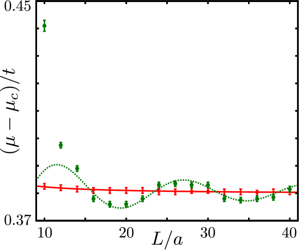
The expressions for the topological invariant given in terms of the scattering matrix in Sec. IV do not coincide with $\mathcal{Q}(H)$ very close to the transition. This is a finite size effect. In order to estimate the importance of finite size effects we have computed the shift of the transition point between the $n=0$ and $n=1$ plateaus of a disordered quantum Hall system as a function of size. We have used a square lattice discretization (lattice constant $a$) of a single band tight binding model with nearest neighbor hopping $t=1$. The magnetic flux per unit cell of the lattice was fixed at $0.4\hbar/e$. We used on-site disorder homogeneously distributed on an interval $[-0.05,0.05]$.

The transition point is defined as the value of the chemical potential $\mu_{c}$ at which the disorder-averaged topological invariant equals 0.5. We have compared two expressions for the topological invariant: the scattering matrix expression (35) and the Hamiltonian expression from Ref. Loring and Hastings, 2010. The results are shown in Fig. 4. We fit the data obtained via the scattering matrix approach to the function $f(L)=c_{1}+c_{2}/L$ obtaining a value $c_{2}\approx 0.026$. In the case of the expression of Ref. Loring and Hastings, 2010, the finite size effect are best fit to the function $g(L)=c_{1}^{\prime}+c_{2}^{\prime}\sin(c_{3}L+c_{4})/L$, with $c_{2}^{\prime}\approx 0.116$. We conclude that the finite size effects of our algorithm are significantly lower.

V.3 Applications

Figure 5: Top panel: Evolution of the poles (green dots) and the zeros (red dots) of $\det r(z)$ as a function of a parameter $\alpha$ which tunes through the topological phase transition in classes A, AII, and DIII in 2D. Shown is the complex plane with the unit circle $|z|=1$ indicated in blue. Time-reversal symmetry in AII and DIII implies that for every zero/pole at $z_{0}$ there is additionally one at $1/z_{0}$. In DIII, there is additional particle-hole symmetry which additionally dictates zeros/poles at $z_{0}^{*}$ and $1/z_{0}^{*}$.The phase transition happens when at least one of the zeros crosses the unit circle. This event coincides with a change of the topological invariant $\mathcal{Q}$ (green) defined by Eqs. (35 – 37)

, as shown in the bottom panels.

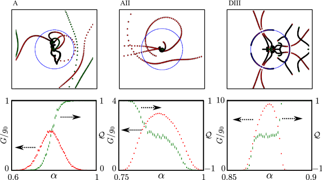
In 2D we illustrate our approach by applying it to network models in classes A, AII, and DIII. In class A we use the Chalker-Coddington network model.Chalker and Coddington (1988) In classes AII and DIII we have used the quantum spin Hall network model of Ref. Ryu et al., 2010b. In class DIII we have set the link phases to zero in order to ensure particle-hole symmetry. In each of these cases the parameter which tunes through the transition is the angle $\alpha$ related to reflection probability at a node of the network by $R=\cos^{2}\alpha$.

Our results are summarized in Fig. 5. Top panels show the evolution of zeros and poles of $\det r(z)$ across the phase transition — the ‘fingerprint’ of a topological phase transition.mov There are no symmetry constraints on this fingerprint in class A. The time-reversal symmetry ensures that for every zero or pole at $z_{0}$ there is another one at $1/z_{0}$. The particle-hole symmetry translates into the mirror symmetry with respect to the real axis: for every zero or pole at $z_{0}$ there is one at $z_{0}^{*}$. The bottom panels show the behavior of the topological invariant and of the conductance $G=\operatorname{tr}t^{\dagger}t$, with $t$ the transmission matrix through the system. The simulations were performed on systems of size $300\times 300$ in each of the symmetry classes and averaged over 1000 samples. The presence of plateaus around zero in the curves for the topological invariant coincides with the presence of a metallic phase in the phase diagram of symmetry classes AII and DIII.

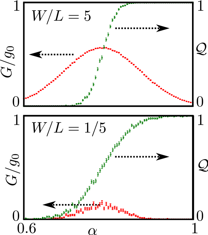
Although we introduced the topological invariant through transport properties, it does not always have the same features as the conductance. The topological invariant characterizes winding of scattering modes in the transverse direction. Accordingly, in a system with a large ratio of width $W$ to the length $L$, the width of the transition of the topological invariant is reduced. The width of the peak in the conductance, on the contrary, is reduced if $W/L$ becomes small. This is in agreement with what we observe in numerical simulations. We have calculated the topological invariant and conductance averaged over 1000 disorder realizations in the Chalker-Coddington network model in systems with $W=300$ and $L=60$ and vice versa. The results are shown in Fig. 6 and they agree with our expectations.

Figure 6: Average topological invariant $\mathcal{Q}$ (35) and longitudinal conductance $G$ of a disordered quantum Hall sample for different aspect ratios as a function of the mixing angle $\alpha$.

Figure 7: Conductance and topological invariant (39) for a disordered 3D topological insulator in class AII.

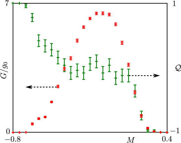
We have also studied a 3D topological system in class AII on a cubic lattice. We have used a simplified version of the Hamiltonian of Ref. Zhang et al., 2009:

$$H=\begin{pmatrix}{\cal M}({\bf k})&vk_{z}&0&vk_{-}\\ vk_{z}&-{\cal M}({\bf k})&vk_{-}&0\\ 0&vk_{+}&{\cal M}({\bf k})&-vk_{z}\\ vk_{+}&0&-vk_{z}&-{\cal M}({\bf k})\end{pmatrix}-\mu$$ (43)

discretized on cubic lattice with lattice constant $a$, where $k_{\pm}=k_{x}\pm ik_{y}$, and ${\cal M}({\bf k})=M-\alpha k^{2}$. The Hamiltonian parameters were chosen to be $\alpha=a^{2}$, $v=a$. We chose $\mu=\mu_{0}+\delta\mu$ with $\mu_{0}=0.4$, and $\delta\mu$ being a random uncorrelated variable uniformly distributed in the interval $[-2,2]$. The topological invariant defined by Eq. (39) as well as the longitudinal conductance for a $20\times 20\times 20$ system averaged over 100 disorder realizations are shown in Fig. 7 as a function of $M$. We observe that, analogously to the two-dimensional case, the presence of a metallic phase is accompanied by a plateau in the topological charge at a value of zero.

VI Conclusion

In conclusion, we have introduced a procedure of dimensional reduction which relates a scattering matrix of a $d$-dimensional system to a Hamiltonian in $d-1$ dimensions with a different symmetry class, but with the same topological invariant as the original system. When applied repeatedly this dimensional reduction procedure serves as an alternative derivation of the Bott periodicity of topological insulators and superconductors.

Since our approach uses only Fermi surface properties it is much more efficient than existing alternatives which require the analysis of the full spectrum. We have described how to implement our method efficiently in all the symmetry classes in 1–3 dimensions. We have verified that it allows to analyze much larger systems than previously possible.

This paper focused on the description of the method and we only touched on a few applications at the end. More applications can be envisaged and we believe that the scattering approach will lead to the discovery of new observable physics at topological phase transitions.

Appendix A Introduction to discrete symmetries

Here we define the three core discrete symmetries, and the corresponding symmetry constraints on the Hamiltonians and on the scattering matrices. We also specify how to choose the symmetry representation we used in Fig. 2.

Definitions and properties of discrete symmetries

The discrete symmetries are defined as follows: The time reversal symmetry operator $\mathcal{T}$ is an anti-unitary operator. When it is applied to an arbitrary eigenstate $\psi$ of the Hamiltonian $H$ at energy $\varepsilon$, returns an eigenstate of the Hamiltonian at the same energy:

$$H\psi=\varepsilon\psi\Rightarrow H\mathcal{T}\psi=\varepsilon\mathcal{T}\psi$$ (44a)

On the other hand, the anti-unitary particle-hole symmetry operator $$\mathcal{P}$$ returns an eigenstate with opposite energy when applied to any eigenstate of the Hamiltonian:

$$H\psi=\varepsilon\psi\Rightarrow H\mathcal{P}\psi=-\varepsilon\mathcal{P}\psi$$ (44b)

Chiral symmetry $$\mathcal{C}$$ also reverses energy, but unlike the other two has a unitary operator.

All three symmetries $\mathcal{T},\mathcal{P},\mathcal{C}$ are $\mathbb{Z}_{2}$ symmetries, so the symmetry operators must square to a phase factor.

In an arbitrary basis the symmetry operators are represented by

$${\cal T}=U^{\hphantom{{\dagger}}}_{\cal T}{\cal K},\quad{\cal P}=U^{\hphantom{{\dagger}}}_{\cal P}{\cal K},\quad{\cal C}=U^{\hphantom{{\dagger}}}_{\cal C},$$ (45)

with $\mathcal{K}$ denoting the complex conjugation, and $U_{\mathcal{T}}$, $U_{\mathcal{P}}$, and $U_{\mathcal{C}}$ unitary matrices. Since $\exp(i\phi)=\mathcal{T}^{2}=U_{\mathcal{T}}U_{\mathcal{T}}^{*}$, and its determinant $\det U_{\mathcal{T}}U_{\mathcal{T}}^{*}$ is real, we obtain $U_{\mathcal{T}}U_{\mathcal{T}}^{*}=\pm 1$; similarly $U_{\mathcal{P}}U_{\mathcal{P}}^{*}=\pm 1$. In other words, every anti-unitary symmetry comes in two flavors, squaring either to $+1$ or to $-1$. No such constraint applies to chiral symmetry, which may square to an arbitrary phase factor $\exp(i\phi)$. This factor however can always be set to zero by choosing $U_{\mathcal{C}}\rightarrow U_{\mathcal{C}}\exp(-i\phi/2)$.

The symmetry constraints on the Hamiltonian

$$H ={\cal T}H{\cal T}^{-1}=U_{\cal T}^{\hphantom{{\dagger}}}H^{*}U^{\dagger}_{\cal T}$$ (46a)

$$H =-{\cal P}H{\cal P}^{-1}=-U_{\cal P}^{\hphantom{{\dagger}}}H^{*}U^{\dagger}_{\cal P}$$ (46b)

$$H =-{\cal C}H{\cal C}^{-1}=-U^{\hphantom{{\dagger}}}_{\cal C}HU_{\cal C}^{\dagger}.$$ (46c)

follow immediately from the definition of the symmetries, Eq. (44).

Relation between discrete symmetries and translational invariance

In addition to the basic properties, the discrete symmetries in periodic systems are required to commute with the coordinate operator. So for any Bloch wave written as

$$\psi(\bm{r})=e^{i\bm{p}\bm{r}}\psi(0),$$ (47)

with $\bm{r}$ coordinate in a translationally-invariant system, and $\psi(0)$ the wave function inside a single unit cell, the action of the symmetry operators is:

$$\mathcal{T}\psi(\bm{r}) =e^{-i\bm{p}\bm{r}}\mathcal{T}\psi(0),$$ (48a)

$$\mathcal{P}\psi(\bm{r}) =e^{-i\bm{p}\bm{r}}\mathcal{P}\psi(0),$$ (48b)

$$\mathcal{C}\psi(\bm{r}) =e^{i\bm{p}\bm{r}}\mathcal{C}\psi(0).$$ (48c)

Since the velocity of a Hamiltonian eigenstate at energy $\varepsilon$ and momentum $\bm{p}$ is $v=d\varepsilon/d\bm{p}$, time-reversal and chiral symmetries reverse the velocity, while particle-hole symmetry keeps the velocity invariant.

Symmetry constraints on scattering matrix

In order to figure out what the symmetry constraints on the scattering matrices are, we first review the basic properties of the scattering matrices. Scattering matrices act in the space of asymptotic scattering states outside of the scattering region. This space contains two non-intersecting subspaces: the subspace of incoming modes and the subspace of outgoing modes. The incoming modes are all the plane waves with velocity in the direction of the scattering region, and the outgoing modes are all the plane waves with velocity pointing away from the scattering region. Let $\psi_{n}^{\text{in}}$ be a basis in the space of incoming modes, and $\psi_{n}^{\text{out}}$ a basis in the space of outgoing modes. Conventionally all the modes are normalized such that current operator in the basis of $\psi^{\text{in}}$ is the identity matrix, and the negative identity matrix in the basis of $\psi^{\text{out}}$.

The matrix elements of the scattering matrix $S$ satisfy

$$(H-\varepsilon)\left(\psi_{n}^{\text{in}}+\sum_{m}S_{mn}\psi_{m}^{\text{out}}+\psi^{\text{loc}}\right)=0,$$ (49)

with $\psi^{\text{loc}}$ a wave-function localized near the scattering region.

As derived in the previous subsection, time-reversal and chiral symmetries change the velocity to its opposite, while particle-hole symmetry leaves the velocity invariant. This means that scattering states transform under the discrete symmetries in the following manner:

$$\mathcal{T}\psi_{n}^{\text{in}} = \sum_{m}\left(V_{\mathcal{T}}\right)_{nm}\psi_{m}^{\text{out}},$$ (50)

$$\mathcal{T}\psi_{n}^{\text{out}} = \sum_{m}\left(Q_{\mathcal{T}}\right)_{nm}\psi_{m}^{\text{in}},$$

$$\mathcal{C}\psi_{n}^{\text{in}} = \sum_{m}\left(V_{\mathcal{C}}\right)_{nm}\psi_{m}^{\text{out}},$$

$$\mathcal{C}\psi_{n}^{\text{out}} = \sum_{m}\left(Q_{\mathcal{C}}\right)_{nm}\psi_{m}^{\text{in}},$$

$$\mathcal{P}\psi_{n}^{\text{out}} = \sum_{m}\left(V_{\mathcal{P}}\right)_{nm}\psi_{m}^{\text{out}},$$

$$\mathcal{P}\psi_{n}^{\text{in}} = \sum_{m}\left(Q_{\mathcal{P}}\right)_{nm}\psi_{m}^{\text{in}}.$$

The additional constraints on the type of time-reversal, particle-hole, and chiral symmetries require

$$\pm 1 = \mathcal{T}^{2}=V_{\mathcal{T}}Q_{\mathcal{T}}^{*},$$ (51a)

$$\pm 1 = \mathcal{P}^{2}=V_{\mathcal{P}}V_{\mathcal{P}}^{*}=Q_{\mathcal{P}}Q_{\mathcal{P}}^{*},$$ (51b)

$$1 = \mathcal{C}^{2}=V_{\mathcal{C}}Q_{\mathcal{C}}.$$ (51c)

Applying time-reversal symmetry to Eq. (49) and using Eqs. (50) we get

$$(H-\varepsilon)\left(V_{\mathcal{T}}\psi_{n}^{\text{out}}+\sum_{m}S_{mn}^{*}Q_{\mathcal{T}}\psi_{m}^{\text{in}}+\mathcal{T}\psi^{\text{loc}}\right)=0,$$ (52)

where we have also used that $H$ is time-reversal invariant. Comparing with Eq. (49), we get

$$S^{-1}=Q_{\mathcal{T}}^{T}S^{*}V_{\mathcal{T}},$$ (53)

which we can be reduced to

$$S=V_{\mathcal{T}}^{T}S^{T}Q_{\mathcal{T}}^{*}.$$ (54a)

Similarly, the chiral and the particle-hole symmetry constraints on $$S$$ are:

$$S =V_{\mathcal{C}}^{T}S^{\dagger}V_{\mathcal{C}}^{T},$$ (54b)

$$S =V_{\mathcal{P}}^{T}S^{*}Q_{\mathcal{P}}^{*}.$$ (54c)

Naturally, the constraints imposed by chiral and particle-hole symmetry only hold at zero excitation energy, since these symmetries anti-commute with the Hamiltonian. Finally, the symmetry constraints on the reflection matrix are identical to Eqs. (54), since $r$ is a diagonal sub-block of $S$.

Choice of symmetry representation and mapping from scattering matrix to Hamiltonian symmetries

The choice of symmetry representation is fully specified by choice of unitary matrices $U_{\mathcal{O}}$, $V_{\mathcal{O}}$, and $Q_{\mathcal{O}}$ ($\mathcal{O}=\mathcal{T},\mathcal{P},\text{ or }\mathcal{C}$). The symmetry representations used in the main text were chosen to make the mapping from the reflection matrix to an effective Hamiltonian most straightforward. In order to reach this aim, we always choose $V_{\mathcal{O}}=\pm Q_{\mathcal{O}}$ for each of the three symmetries. Whenever chiral symmetry is present, we use

$$U_{\mathcal{C}}=\tau_{z},\quad V_{\mathcal{C}}=Q_{\mathcal{C}}=1.$$ (55)

Our choices of $V$ and $Q$ for the other two symmetries with

$$V_{\mathcal{T}}=V_{\mathcal{P}}\equiv V,\quad Q_{\mathcal{T}}=Q_{\mathcal{P}}\equiv Q$$ (56)

depend on the specific symmetry class. When $\mathcal{P}^{2}=-1$ (symmetry classes C, CI, CII) we choose $V=\sigma_{y}$, and we choose $V=1$ in symmetry classes D, DIII, and BDI, where $\mathcal{P}^{2}=1$. The relative sign between $V$ and $Q$ follows from Eq. (51):

$$Q=\mathcal{P}^{2}\mathcal{T}^{2}V.$$ (57)

In the remaining two classes AI and AII we choose $V=1$, and $Q=\mathcal{T}^{2}$. Symmetry representations of the effective Hamiltonians follow immediately from Eqs. (21).

Finally we show how symmetry operators change upon creating an effective Hamiltonian from a reflection matrix. The effective Hamiltonian created from a reflection matrix with chiral symmetry satisfies

$$H=\mathcal{P}^{2}\mathcal{T}^{2}VH^{*}V,$$ (58)

so that the resulting symmetry of the effective Hamiltonian is particle-hole if $\mathcal{P}^{2}\mathcal{T}^{2}=-1$, and time-reversal if $\mathcal{P}^{2}\mathcal{T}^{2}=1$. The symmetry operator of this symmetry squares to $VV^{*}$. If a reflection matrix has only time-reversal symmetry, then the time-reversal and particle-hole symmetry constraints on the effective Hamiltonian have the form

$$H=\pm V\otimes\tau_{x}H^{*}V\otimes\tau_{x},$$ (59a)

$$H=\mp V\otimes\tau_{y}H^{*}V\otimes\tau_{y},$$ (59b)

where the sign is determined by the choice of representation of the symmetry of $r$. Hence the symmetries of the effective Hamiltonian satisfy $\mathcal{T}^{2}=-\mathcal{P}^{2}$. Finally, for an effective Hamiltonian constructed from a reflection matrix with only particle-hole symmetry, the resulting symmetry constraints on the Hamiltonian are

$$H=\pm V\otimes\tau_{0}H^{*}V\otimes\tau_{0},$$ (60a)

$$H=\mp V\otimes\tau_{z}H^{*}V\otimes\tau_{z},$$ (60b)

so that both symmetry operators square to the same value.

Appendix B Calculation of the number of poles of $\bm{\det r(z)}$ inside the unit circle

We prove that the equation

$$\det[A-Z_{1}(k)]=0$$ (61)

has $N_{1}$ solutions with $z=e^{ik}$ inside the unit circle, and $N_{1}$ solutions outside of the unit circle as long as $A^{\dagger}A$ only has eigenvalues less than one, which is generically the case since $A$ is a sub-block of a unitary matrix $S$. Let us assume that $\psi$ is an eigenvector of the corresponding eigenvalue problem:

$$A\psi=Z_{1}(k)\psi,$$ (62)

with an eigenvalue with $|z|=1$. In this case $Z^{\dagger}_{1}(k)Z_{1}(k)=1$. We come to a contradiction by considering the following inequality:

$$\psi^{\dagger}\psi>\psi^{\dagger}A^{\dagger}A\psi=\psi^{\dagger}Z^{\dagger}_{1}(k)Z_{1}(k)\psi=\psi^{\dagger}\psi$$ (63)

So we conclude that there are no solutions of $\det[A-Z_{1}(k)]=0$ with $z$ on the unit circle. Next, we observe that for $A=0$ there are exactly $N_{1}$ of $\det[A-Z_{1}(k)]=0$ with $z=0$ and $N_{1}$ solutions with $z=\infty$. Since these solutions never cross the unit circle when $A$ is smoothly deformed, we come to the statement we set to prove.

References

- Altland and Zirnbauer (1997) A. Altland and M. R. Zirnbauer, Phys. Rev. B 55, 1142 (1997).
- Kitaev (2009) A. Kitaev, AIP Conf. Proc. 1134, 22 (2009).
- Schnyder et al. (2009) A. P. Schnyder, S. Ryu, A. Furusaki, and A. W. W. Ludwig, AIP Conf. Proc. 1134, 10 (2009).
- Loring and Hastings (2010) T. A. Loring and M. B. Hastings, Europhys. Lett. 92, 67004 (2010).
- Ringel and Kraus (2011) Z. Ringel and Y. E. Kraus, Phys. Rev. B 83, 245115 (2011).
- Hastings and Loring (2011) M. B. Hastings and T. A. Loring, Ann. Phys. 326, 1699 (2011).
- Fulga et al. (2011) I. C. Fulga, F. Hassler, A. R. Akhmerov, and C. W. J. Beenakker, Phys. Rev. B 83, 155429 (2011).
- Akhmerov et al. (2011) A. R. Akhmerov, J. P. Dahlhaus, F. Hassler, M. Wimmer, and C. W. J. Beenakker, Phys. Rev. Lett. 106, 057001 (2011).
- Wimmer et al. (2011) M. Wimmer, A. R. Akhmerov, J. P. Dahlhaus, and C. W. J. Beenakker, New J. Phys. 13, 053016 (2011).
- Qi et al. (2008) X.-L. Qi, T. L. Hughes, and S.-C. Zhang, Phys. Rev. B 78, 195424 (2008).
- Ryu et al. (2010a) S. Ryu, C. Mudry, H. Obuse, and A. Furusaki, New J. Phys. 12, 065005 (2010a).
- Thouless et al. (1982) D. J. Thouless, M. Kohmoto, M. P. Nightingale, and M. den Nijs, Phys. Rev. Lett. 49, 405 (1982).
- Halperin (1982) B. I. Halperin, Phys. Rev. B 25, 2185 (1982).
- Büttiker (1988) M. Büttiker, Phys. Rev. B 38, 9375 (1988).
- Laughlin (1981) R. B. Laughlin, Phys. Rev. B 23, 5632 (1981).
- Büttiker et al. (1994) M. Büttiker, H. Thomas, and A. Prêtre, Z. Phys. B Cond. Mat. 94, 133 (1994).
- Brouwer (1998) P. W. Brouwer, Phys. Rev. B 58, R10135 (1998).
- Bräunlich et al. (2010) G. Bräunlich, G. M. Graf, and G. Ortelli, Commun. Math. Phys. 295, 243 (2010).
- Zak (1989) J. Zak, Phys. Rev. Lett. 62, 2747 (1989).
- Ryu and Hatsugai (2002) S. Ryu and Y. Hatsugai, Phys. Rev. Lett. 89, 077002 (2002).
- Mahaux and Weidenmüller (1969) C. Mahaux and H. A. Weidenmüller, Shell-Model Ap- proach to Nuclear Reactions (North-Holland, Amsterdam, 1969).
- Stone et al. (2011) M. Stone, C.-K. Chiu, and A. Roy, J. Phys. A: Math. Theor. 44, 045001 (2011).
- Teo and Kane (2010) J. C. Y. Teo and C. L. Kane, Phys. Rev. B 82, 115120 (2010).
- Kitaev (2001) A. Y. Kitaev, Phys.-Usp. 44, 131 (2001).
- Qi et al. (2010) X.-L. Qi, T. L. Hughes, and S.-C. Zhang, Phys. Rev. B 81, 134508 (2010).
- Fu and Kane (2006) L. Fu and C. L. Kane, Phys. Rev. B 74, 195312 (2006).
- Meidan et al. (2011a) D. Meidan, T. Micklitz, and P. W. Brouwer, Phys. Rev. B 84, 075325 (2011a).
- Meidan et al. (2011b) D. Meidan, T. Micklitz, and P. W. Brouwer, Phys. Rev. B 84, 195410 (2011b).
- Ryu et al. (2012) S. Ryu, J. E. Moore, and A. W. W. Ludwig, Phys. Rev. B 85, 045104 (2012).
- Wang et al. (2011) Z. Wang, X.-L. Qi, and S.-C. Zhang, Phys. Rev. B 84, 014527 (2011).
- Prodan (2011a) E. Prodan, J. Phys. A: Math. Theor. 44, 113001 (2011a).
- Loring and S rensen (2011) T. A. Loring and A. P. W. S rensen, arXiv:1107.4187 (2011).
- Hasan and Kane (2010) M. Z. Hasan and C. L. Kane, Rev. Mod. Phys. 82, 3045 (2010).
- Fu et al. (2007) L. Fu, C. L. Kane, and E. J. Mele, Phys. Rev. Lett. 98, 106803 (2007).
- Moore and Balents (2007) J. E. Moore and L. Balents, Phys. Rev. B 75, 121306 (2007).
- Schnyder and Ryu (2011) A. P. Schnyder and S. Ryu, Phys. Rev. B 84, 060504 (2011).
- Wan et al. (2011) X. Wan, A. M. Turner, A. Vishwanath, and S. Y. Savrasov, Phys. Rev. B 83, 205101 (2011).
- George (1973) A. George, SIAM J. Numer. Anal. 10, 345 (1973).
- Li et al. (2008) S. Li, S. Ahmed, G. Klimeck, and E. Darve, J. Comp. Phys. 227, 9408 (2008).
- Wimmer (2012) M. Wimmer, ACM Trans. Math. Softw. 38, 30 (2012).
- Bernevig et al. (2006) B. A. Bernevig, T. L. Hughes, and S.-C. Zhang, Science 314, 1757 (2006).
- Prodan (2011b) E. Prodan, Phys. Rev. B 83, 195119 (2011b).
- Chalker and Coddington (1988) J. T. Chalker and P. D. Coddington, J. Phys. C: Solid State Phys. 21, 2665 (1988).
- Cho and Fisher (1997) S. Cho and M. P. A. Fisher, Phys. Rev. B 55, 1025 (1997).
- Ryu et al. (2010b) S. Ryu, A. P. Schnyder, A. Furusaki, and A. W. W. Ludwig, New J. Phys. 12, 065010 (2010b).
- (46) The Supplemental Material at http://arxiv.org/src/1106.6351/anc shows movies of this ‘fingerprint’ in classes A, AII, and DIII.
- Zhang et al. (2009) H. Zhang, C.-X. Liu, X.-L. Qi, X. Dai, Z. Fang, and S.-C. Zhang, Nat. Phys. 5, 438 (2009).