Practical and accurate calculations of Askaryan radiation.

Abstract

An in-depth characterization of coherent radio Cherenkov pulses from particle showers in dense dielectric media, referred to as the Askaryan effect, is presented. The time-domain calculation developed in this article is based on a form factor to account for the lateral dimensions of the shower. It is computationally efficient and able to reproduce the results of detailed particle shower simulations with high fidelity in most regions of practical interest including Fresnel effects due to the longitudinal development of the shower. In addition, an intuitive interpretation of the characteristics of the Askaryan pulse is provided. We expect our approach to benefit the analysis of radio pulses in experiments exploiting the radio technique.

I Introduction

In 1962 Askaryan Askaryan62 proposed to detect Ultra-High Energy (UHE) cosmic rays and neutrinos observing the coherent radio pulse from the excess of electrons in a shower developing in a dense dielectric and non-absorptive medium. The scaling of the emitted power with the square of the particle energy, which has been experimentally confirmed in accelerators Saltzberg_SLAC_sand ; Miocinovic_SLAC_sand ; Gorham_SLAC_salt ; Gorham_SLAC_ice , makes the technique very promising for the detection of UHE particles and has motivated a variety of past and present experiments Parkes96 ; RICE03 ; GLUElimits ; NuMoon ; Kalyazin ; ANITA_2009_limits ; LUNASKA ; RESUN along with some in the planning stages ARA ; ARIANNA .

Key to the success of these initiatives is an accurate and computationally efficient calculation of the radio emission properties due to the Askaryan effect in UHE showers. The problem of computing the coherent radiation from particle showers can be approached in a variety of ways. Purely Monte Carlo methods have been developed to simulate the induced showers in dense media. One can obtain the contribution to the radiation from every particle track in the shower from first principles (Maxwell’s equations), and add the contributions, which automatically takes coherent effects into account. This approach has been applied to calculate the Fourier components of the radiation (i.e. in the frequency-domain) ZHS91 ; ZHS92 ; alz97 ; alz98 ; alvz99 ; alvz00 ; razzaque01 ; almvz03 ; razzaque04 ; McKay_radio ; alvz06 ; aljpz09 ; zhaires10 , and only recently to the calculation of the radiation as a function of time (i.e. in the time-domain) ARZ10 . Similar methods have also been applied to the calculation of radio emission in atmospheric showers ReAires ; Konstantinov ; REAS3 ; SEIFAS ; zhaires_nantes ; zhaires_air11 ; SEIFAS in which the Askaryan effect is not the dominant mechanism and will not be addressed in this paper. Monte Carlo methods have the advantage that the full complexity of shower phenomena is accounted for, the influence of shower-to-shower fluctuations can be addressed, and the dependence on the type of primary particle, hadronic model, along with any other assumptions can be studied with high accuracy. However, purely Monte Carlo methods are typically very time-consuming, especially at ultra-high energies and approximations are required aljpz09 .

Another numerical approach currently being developed is the application of finite difference in the time-domain (FDTD) techniques Chih10 . The idea is to discretize space-time and propagate the electric and magnetic fields by approximation of Maxwell’s differential equations into difference equations FDTDbook . FDTD techniques have the advantage that they can be easily adapted to computing the effects of dielectric boundaries and index of refraction gradients and can be linked to an accurate Monte Carlo simulation of showers in dense media. The FDTD technique is however rather computationally intensive Chih10 .

Analytical approaches have also been developed. In these methods the charge development in the shower is approximated as a current density vector buniy02 . Typically, parameterizations of the longitudinal and lateral profile of the showers are used to describe the main features of the space-time evolution of the charge distribution. In this approach one calculates the vector potential by integrating the Green’s function to obtain the electric field. These integrals are in general difficult both numerically and analytically, but they can be greatly simplified by the use of approximations buniy02 . These methods are usually less time-consuming but also less accurate than purely Monte Carlo simulations. One limitation is that showers elongated due to the Landau-Pomeranchuk-Migdal (LPM) effect LPM ; Stanev_LPM cannot be parameterized easily due to large shower-to-shower fluctuations and the emitted radiation is known to depend strongly on the particular longitudinal profile of the shower alz97 ; alz98 ; alvz99 . Analytical techniques have also been applied with different levels of sophistication to the calculation of radio emission in atmospheric showers Huege_analytical ; Scholten_MGMR ; Montanet_radio ; Ardouin_Coulomb .

It is clearly important to be able to calculate coherent radiation due to the Askaryan as well as other effects with a variety of techniques as each has its own set of advantages and disadvantages. Our goal in this work is to provide a calculation method that is both fast and able to reproduce all the essential characteristics resulting from detailed Monte Carlo shower simulations. Semi-analytical techniques are a very good option. The general idea behind this method is to obtain the charge distribution from detailed Monte Carlo simulations as the input for an analytical calculation of the radio pulse. Other semi-analytical methods in dense media alz97 ; alz98 ; alvz99 ; ARZ10 and in the atmosphere Scholten_MGMR_sims have been attempted in the past. In dense media, the frequency spectrum of the radio emission due to the Askaryan effect has been shown to be easily obtained from the Fourier-transform of the longitudinal profile of the shower alvz99 . This technique reproduced the frequency spectrum as predicted in Monte Carlo simulations with a high degree of accuracy, but only for angles away from the Cherenkov angle in the Fraunhofer approximation. Complementary, in the time-domain, it was shown that the electric field away from the Cherenkov angle and in the far-field regime can be very accurately calculated from the time-derivative of the simulated longitudinal development of the excess charge ARZ10 (see also Scholten_MGMR ).

This paper presents a semi-analytical calculation that is able to reproduce the electric field in the time-domain at all angles with respect to the shower axis in both the far-field (Fraunhofer) and “near-field” regions of the shower when compared to a full Monte Carlo simulation such as the well-known Zas-Halzen-Stanev (ZHS) code ZHS92 ; ARZ10 ; ZHSinprep . The technique is computationally efficient since it only requires the convolution of the longitudinal charge excess profile with a parameterized form factor to fully reproduce the coherent radiation effects from particle showers in a homogeneous dielectric medium. Once the longitudinal shower profile is obtained, the electric field can be calculated with a simple numerical integral. It is worth remarking here that the longitudinal development of extremely energetic showers can be obtained quickly and with high precision, using hybrid simulation techniques which consist on following only the highest energy particles in the shower while accounting for the lowest energy particles with parameterizations. In particular, the complexity of the longitudinal profile of showers affected by the LPM effect can be very well reproduced with hybrid techniques alz97 ; alz98 ; alvz99 (for an example see Fig. $5$ in aljpz09 ).

The semi-analytical method described in this work is well suited to obtain the time-domain radio emission due to electromagnetic showers, for all observation angles both in the far-field and the near-field regions of the shower. The approach can be used in practically all experimental situations of interest since it only begins to show significant discrepancies when the observer is at distances comparable to the lateral dimensions of the shower ($\lesssim$ 1 m in ice). Since the typical distance between antennas in experiments such as the Askaryan Radio Array (ARA) ARA is $\sim 10-100$ m, we expect the results to be accurate enough in most practical situations.

We expect our results to benefit experiments exploiting the radio technique. They can be used in detector simulations to test the efficiency for pulses observed from various directions. In particular, with our approach one can test the ability to detect the craggy pulses resulting from the LPM effect. The calculation can also be implemented in the data analysis of experiments by using likelihood functions aimed at the reconstruction of the longitudinal charge excess profile from a detected pulse. If the longitudinal distribution is consistent with the elongation and multiple-peaked structure due to the LPM effect, this can be used for neutrino flavor identification since it is only expected in UHE showers due to electron neutrinos.

II Modeling Askaryan radiation

The case we are interested in this paper is the radiation due to the charge excess of a shower in a linear dielectric medium such as ice, salt, or silica sand. We use SI units all throughout this work. The Green’s function solutions to Maxwell’s equations provide the potentials $\Phi$ and $\mathbf{A}$ given a charge distribution $\rho$ with current density vector $\mathbf{J}=\rho\mathbf{v}$. Assuming a dielectric constant $\epsilon$ and magnetic constant $\mu$ the solutions in the Coulomb gauge ($\nabla\cdot\mathbf{A}=0$) can be written as

$$\Phi(\mathbf{x},t)=\frac{1}{4\pi\epsilon}\int_{-\infty}^{\infty}\frac{\rho(\mathbf{x}^{\prime},t)}{|\mathbf{x}-\mathbf{x}^{\prime}|}d^{3}\mathbf{x}^{\prime}$$ (1)

$$\mathbf{A}(\mathbf{x},t)=\frac{\mu}{4\pi}\int_{-\infty}^{\infty}\frac{\mathbf{J}_{\perp}(\mathbf{x}^{\prime},t^{\prime})}{|\mathbf{x}-\mathbf{x}^{\prime}|}\delta\left(\sqrt{\mu\epsilon}|\mathbf{x}-\mathbf{x}^{\prime}|-(t-t^{\prime})\right)d^{3}\mathbf{x}^{\prime}dt^{\prime}$$ (2)

where the delta function gives the observer’s time $t$ delayed with respect to the source time $t^{\prime}$ by the time it takes light to reach the observation point $\mathbf{x}$ from the source position at $\mathbf{x}^{\prime}$. The transverse current is given by $\mathbf{J}_{\perp}=-\mathbf{\hat{u}}\times\-(\mathbf{\hat{u}}\times\mathbf{J})$ where $\mathbf{\hat{u}}=(\mathbf{x}-\mathbf{x}^{\prime})/|\mathbf{x}-\mathbf{x}^{\prime}|$ is the unit vector pointing from the source to the observer. The non-trivial proof that the $\mathbf{J}_{\perp}$ above is the only component relevant to the radiation part of the field is given in Jackson_AmJPhys .

Radiation calculations are typically performed in the Lorentz gauge ($\nabla\cdot\mathbf{A}+n^{2}~{}c^{-2}\partial\Phi/\partial t=0$)  Jackson ; buniy02 ; razzaque04 ; Scholten_MGMR , with $n$ the refractive index of the medium. However, our primary interest is to derive an approach that can be easily applied to numerical radiation calculations. In the Coulomb gauge, the scalar potential only describes near-field terms which can be ignored for our purposes. This simplifies the computation of the radiative electric field $\mathbf{E}=-\nabla\Phi-\partial\mathbf{A}/\partial t$ to a simple time derivative $\mathbf{E}=-\partial\mathbf{A}/\partial t$. Thus, all that is needed is a computation of the vector potential as a function of time at the position of interest.

The radiation of a particle shower in a dense medium is obtained by treating it as a current density $\mathbf{J}$ with its main features depicted in Fig.1. The evolution in space-time of the excess charge in a shower can be modeled as a pancake $\delta(z^{\prime}-vt^{\prime})$ traveling with velocity $\mathbf{v}$ along the $z$–axis. The net charge profile of the shower $Q(z^{\prime})$ rises and falls along the shower direction $z^{\prime}$ and spreads laterally in $x^{\prime}$ and $y^{\prime}$. The velocity vector $\mathbf{v}$ is primarily directed in the shower axis direction $\mathbf{\hat{z}}$ but may have a small lateral component and a lateral dependence due to scattering of particles in the shower. This may seem like an unnecessary complication but the small scatter will lead to an observable asymmetry of the Askaryan pulse in the time-domain. The speed $v$ is assumed to be close to the speed of light for particle showers of interest. The associated current density vector can be modeled as a cylindrically symmetric function

$$\mathbf{J}(\mathbf{x}^{\prime},t^{\prime})=\mathbf{v}(r^{\prime},\phi^{\prime},z^{\prime})f(r^{\prime},z^{\prime})Q(z^{\prime})\delta(z^{\prime}-vt^{\prime})$$ (3)

where $r^{\prime}=\sqrt{x^{\prime 2}+y^{\prime 2}}$ is the cylindrical radius. The function $f(r^{\prime},z^{\prime})$ represents the lateral charge distribution in a plane transverse to $z^{\prime}$ depicted in the bottom of Fig. 1. This model of the current density is similar to the ones used in buniy02 ; razzaque04 except that $\mathbf{v}$ is allowed to have first order radial components.

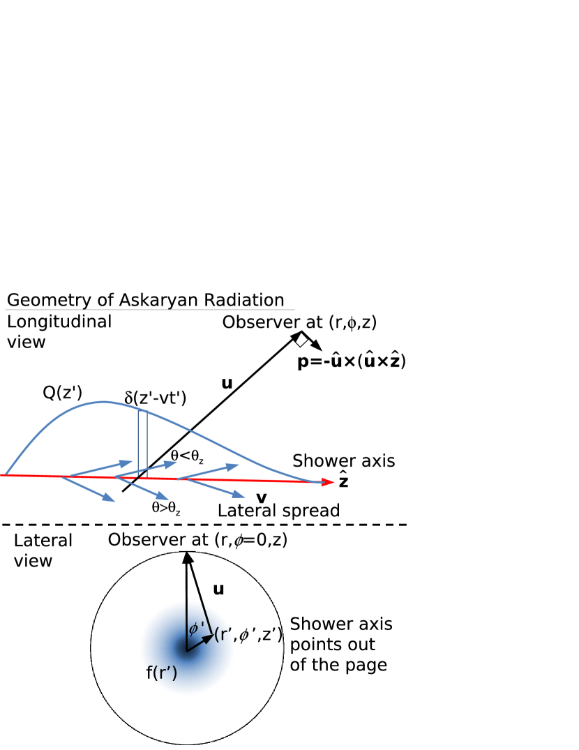
Figure 1: Geometry of a high energy particle shower. The top figure shows a side view ($r-z$ plane) of the charge excess profile. The shower front propagates at velocity $v$ and is modeled as a thin pancake $\delta(z^{\prime}-vt^{\prime})$. The charge evolution of the shower front traces out the longitudinal profile $Q(z^{\prime})$ shown here as an asymmetric distribution. The lateral spread of the shower due to Coulomb scattering, shown in (blue) arrows, is modeled by a velocity vector $\mathbf{v}=\mathbf{v}(r^{\prime},\phi^{\prime})$ that is mostly directed along the shower axis with small radial components. The scatter results in observation angles that differ from the nominal angle $\theta_{z}$ relative to the shower axis and will lead to an asymmetric pulse. The radiative portion of the electric field lies along the vector $\mathbf{p}$ which is the orthogonal projection of $\mathbf{\hat{z}}$ along the direction $\mathbf{\hat{u}}$ from the source to the observer. The bottom panel shows a frontal view ($r-\phi$ plane) of the shower. The lateral charge excess distribution $f(r^{\prime})$ is represented in (blue) shading.

The vector potential is then given by

$$\begin{split}&\mathbf{A}(\mathbf{x},t)=\frac{\mu}{4\pi}\int^{\infty}_{-\infty}dt^{\prime}\int^{\infty}_{-\infty}dz^{\prime}Q(z^{\prime})\delta(z^{\prime}-vt^{\prime})\\ &\int^{\infty}_{0}dr^{\prime}r^{\prime}\int^{2\pi}_{0}d\phi^{\prime}f(r^{\prime},z^{\prime})\mathbf{{v}}_{\perp}(r^{\prime},\phi^{\prime},z^{\prime})\\ &\frac{\delta\left(n|\mathbf{x}-\mathbf{x}^{\prime}|/c-(t-t^{\prime})\right)}{|\mathbf{x}-\mathbf{x}^{\prime}|}\end{split}$$ (4)

where $\phi^{\prime}$ is the azimuthal angle in cylindrical coordinates and $\mathbf{v}_{\perp}(r^{\prime},\phi^{\prime},z^{\prime})$ generally depends on $r^{\prime}$, $\phi^{\prime}$, and $z^{\prime}$.

In its full glory Eq. (4) seems rather intractable. The lateral distribution $f(r^{\prime},z^{\prime})$ is the most difficult part to model. It is for this reason that the semi-analytical models developed in alvz99 and ARZ10 ignored the lateral development of the shower, and hence were not able to accurately describe Askaryan radiation near the Cherenkov angle where the lateral distribution is known to determine the degree of coherence of the emitted radiation ZHS92 . Modeling the radiation due to the lateral distribution of the shower can be attempted using the standard NKG function Greisen60 . However, this parameterization has singularities that make the integrals particularly difficult to solve and interpret, and it assumes constant particle velocities parallel to the shower axis which is not sufficiently accurate as will be shown further below.

In the following we will show that the radiation due to the lateral distribution of the shower can be parameterized, and this parameterization can be used to predict the emitted radiation matching that obtained from the full ZHS simulation ZHS92 ; ARZ10 with great accuracy. Moreover, the lateral distribution of the shower is mainly due to low energy processes such as Coulomb scattering, and as result the shape of the parameterized radiation is independent of shower energy in the energy range of interest as will be shown below. On the other hand, the longitudinal distribution $Q(z^{\prime})$ can change dramatically depending on the energy of the shower due to the LPM effect, and needs to be obtained in a Monte Carlo simulations such as ZHS. We will also show that our calculation of Askaryan radiation works in both the near and far-field approximations, as long as the lateral coordinates are treated in the far-field, i.e. the observation of the shower occurs at a distance larger than its lateral dimensions ($\sim$ 1 m in ice).

II.1 The vector potential at the Cherenkov angle

Let us first consider the Fraunhofer approximation for radiation emitted by a shower. This implies expanding $|\mathbf{x}-\mathbf{x}^{\prime}|$ in Eq. (2) as

$$|\mathbf{x}-\mathbf{x}^{\prime}|\approx R-\mathbf{\frac{x}{|x|}}\cdot\mathbf{x}^{\prime}$$ (5)

where $R=\mathbf{|x|}$. For an observer looking in the direction $\mathbf{\hat{u}}=\mathbf{x/|x|}=(\sin\theta\cos\phi,\sin\theta\sin\phi,\cos\theta)$ in spherical coordinates, and assuming without loss of generality that $\phi=0$, the above expansion can be written as

$$|\mathbf{x}-\mathbf{x}^{\prime}|\approx R-z^{\prime}\cos\theta-r^{\prime}\sin\theta\cos\phi^{\prime}$$ (6)

Approximating the denominator of the vector potential in Eq. (4) by $|\mathbf{x}-\mathbf{x}^{\prime}|\approx R$ but keeping the approximation in Eq. (6) in the argument of the $\delta$-function we get,

$$\begin{split}&\mathbf{A}(\theta,t)=\frac{\mu}{4\pi R}\int^{\infty}_{-\infty}dt^{\prime}\int^{\infty}_{-\infty}dz^{\prime}Q(z^{\prime})\delta(z^{\prime}-vt^{\prime})\\ &\int^{\infty}_{0}dr^{\prime}r^{\prime}\int^{2\pi}_{0}d\phi^{\prime}f(r^{\prime},z^{\prime})\mathbf{{v}}_{\perp}(r^{\prime},\phi^{\prime},z^{\prime})\\ &\delta\left(\frac{n[R-z^{\prime}\cos\theta-r^{\prime}\sin\theta\cos\phi^{\prime}]}{c}-(t-t^{\prime})\right)\end{split}$$ (7)

Integrating over the source time $t^{\prime}$ results in

$$\begin{split}&\mathbf{A}(\theta,t)=\frac{\mu}{4\pi R}\int^{\infty}_{-\infty}dz^{\prime}Q(z^{\prime})\int^{\infty}_{0}dr^{\prime}r^{\prime}f(r^{\prime},z^{\prime})\\ &\int^{2\pi}_{0}d\phi^{\prime}\frac{\mathbf{v}_{\perp}(r^{\prime},\phi^{\prime},z^{\prime})}{v}\\ &\delta\left(z^{\prime}\left[\frac{1}{v}-\frac{n\cos\theta}{c}\right]-\frac{nr^{\prime}\sin\theta\cos\phi^{\prime}}{c}+\frac{nR}{c}-t\right).\end{split}$$ (8)

where $\mathbf{v}_{\perp}(r^{\prime},\phi^{\prime},z^{\prime})=-\mathbf{\hat{u}}\times\mathbf{\hat{u}}\times\mathbf{v}(r^{\prime},\phi^{\prime},z^{\prime})$ is the transverse projection of the unit velocity vector.

In our model we make the assumption that the shape of the lateral density and the particle velocity depend only very weakly on $z^{\prime}$, i.e. $f(r^{\prime},z^{\prime})\simeq f(r^{\prime})$ and $\mathbf{v}(r^{\prime},\phi^{\prime},z^{\prime})\simeq\mathbf{v}(r^{\prime},\phi^{\prime})$. With these approximations Eq. (8) can be written as:

$$\begin{split}&\mathbf{A}(\theta,t)=\frac{\mu}{4\pi R}~{}\sin\theta~{}\int^{\infty}_{-\infty}dz^{\prime}Q(z^{\prime})\\ &\mathbf{F}\left(t-\frac{nR}{c}-z^{\prime}\left[\frac{1}{v}-\frac{n\cos\theta}{c}\right]\right)~{}\end{split}$$ (9)

where we have defined the function $\mathbf{F}$ as:

$$\begin{split}&\mathbf{F}\left(t-\frac{nR}{c}-z^{\prime}\left[\frac{1}{v}-\frac{n\cos\theta}{c}\right]\right)=\\ &\frac{1}{\sin\theta}~{}\int^{\infty}_{0}dr^{\prime}r^{\prime}\int^{2\pi}_{0}d\phi^{\prime}f(r^{\prime})\frac{\mathbf{v}_{\perp}(r^{\prime},\phi^{\prime})}{v}\\ &\delta\left(z^{\prime}\left[\frac{1}{v}-\frac{n\cos\theta}{c}\right]-\frac{nr^{\prime}\sin\theta\cos\phi^{\prime}}{c}+\frac{nR}{c}-t\right)\end{split}$$ (10)

Note that we have explicitly included a factor $\sin\theta$ in Eq. (9) for convenience, anticipating that the radiation is mainly polarized in the direction transverse to the observer’s direction.

The vector function $\mathbf{F}$ contains the radial $r^{\prime}$ and azimuthal $\phi^{\prime}$ integrals and can be considered as an effective form factor that accounts for the lateral distribution of the charged current density, quite analogous to that obtained in the frequency domain in buniy02 .

At the Cherenkov angle we have $1/v-n\cos\theta_{C}/c=0$ and Eq. (9) results in:

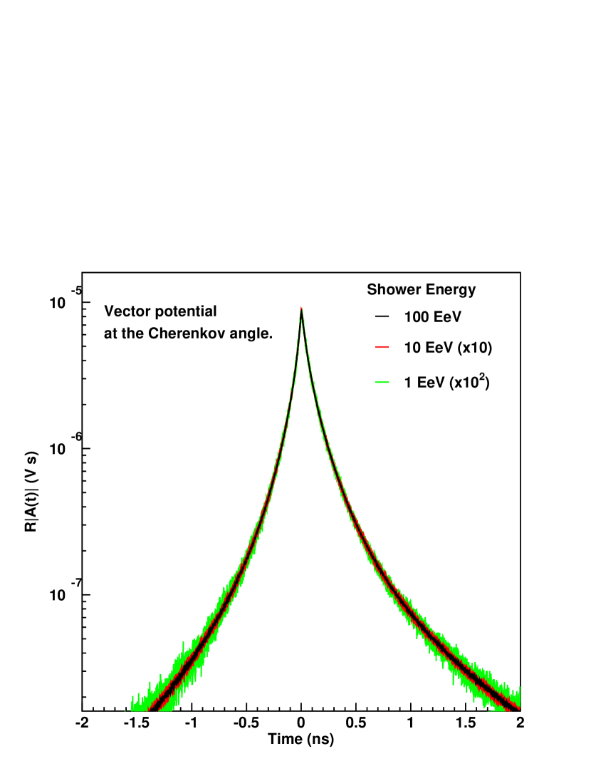
Figure 2: The vector potential from electromagnetic showers in homogeneous ice (density $\rho=0.924~{}{\rm g~{}cm^{-3}}$ and refractive index $n=1.78$, $\theta_{C}\sim 55.8^{\circ}$) observed at the Cherenkov angle for various energies from the ZHS simulation. The functional behavior is identical except for an overall scaling factor that is directly proportional to the shower energy. The width is determined by the lateral distribution of the shower while the asymmetry is mainly due to the radial spread of particle tracks; both are the result of the Coulomb scattering in the medium.

$$\mathbf{A}(\theta_{C},t)=\frac{\mu}{4\pi R}~{}\sin\theta_{C}~{}\mathbf{F}\left(t-\frac{nR}{c}\right)~{}\int^{\infty}_{-\infty}dz^{\prime}Q(z^{\prime})$$ (11)

where $\mathbf{F}$ at the Cherenkov angle is obtained from Eq. (10):

$$\begin{split}&\mathbf{F}\left(t-\frac{nR}{c}\right)=\frac{1}{\sin\theta_{C}}~{}\int^{\infty}_{0}dr^{\prime}r^{\prime}f(r^{\prime})\int^{2\pi}_{0}d\phi^{\prime}\frac{\mathbf{v}_{\perp}(r^{\prime},\phi^{\prime})}{v}\\ &\delta\left(\frac{nR}{c}-t-\frac{nr^{\prime}\sin\theta_{C}\cos\phi^{\prime}}{c}\right).\end{split}$$ (12)

Using symmetry arguments we can now project the form factor $\mathbf{F}$ in only two orthogonal directions using unit vectors $\mathbf{\hat{u}}$ along the observation direction and in the direction of $\mathbf{p}=-\mathbf{\hat{u}}\times(\mathbf{\hat{u}}\times\mathbf{\hat{z}})$:

$$\mathbf{F}=F_{p}~{}\mathbf{\hat{p}}+F_{u}\mathbf{\hat{u}}$$ (13)

The direction of $\mathbf{\hat{p}}$ has been chosen perpendicular to the observation direction and lying on the plane defined by $\mathbf{\hat{z}}$ and $\mathbf{\hat{u}}$ as shown in Fig. 1. This has been done anticipating the expected polarization of the radiation mainly in the direction of $\mathbf{\hat{p}}$ in order to make the orthogonal component along the direction of observation $F_{u}$ negligible.

The form factor $\mathbf{F}$ is a medium dependent function that accounts in an effective way for the radial and azimuthal interference effects due to the lateral structure of the shower including possible directional variations in the velocity vector $\mathbf{v}$ of the shower particles. In principle $\mathbf{F}$ can be obtained from analytical solutions of the cascade equations, but this is rather involved. Alternatively one could use standard parameterizations of the lateral distribution function of high energy showers such as the NKG  Greisen60 . However, as stated before, this does not account for the radial components of the velocity and gives results symmetric in time which are qualitatively different from results obtained in detailed simulations such as that shown in Fig. 2. The trick is to extract $\mathbf{F}$ from simulations that effectively account for the radial component of particle velocities and the lateral distribution of the excess charge which are responsible for the time asymmetry characteristic of simulations. The basic idea behind this article is that the form factor is obtained from the vector potential at the Cherenkov angle and, as we will show later, the emission at other angles is easily related to that at the Cherenkov angle.

The vector potential at the Cherenkov angle in the time domain is calculated with a detailed shower simulation and parameterized for practical purposes. The form factor $\mathbf{F}$ can be obtained directly equating Eq. (11) to the vector potential as obtained in the simulation. As anticipated the $F_{u}$ component is typically below $1~{}\%$ of $F_{p}$ and it can be neglected, and $F_{p}$ can be simply obtained from the following equation:

$$\mathbf{A}(\theta_{C},t)=\frac{\mu}{4\pi R}~{}\sin\theta_{C}~{}F_{p}\left(t-\frac{nR}{c}\right)~{}LQ_{\rm tot}~{}\mathbf{\hat{p}}$$ (14)

where $LQ_{\rm tot}=\int dz^{\prime}Q(z^{\prime})$ has been referred to as the excess projected track-length ZHS92 . Taking the absolute value of Eq. (14) the functional form of $F_{p}$ is given by:

$$F_{p}\left(t-\frac{nR}{c}\right)=\frac{4\pi}{\mu}~{}\frac{RA(\theta_{C},t)}{LQ_{\rm tot}}~{}\frac{1}{\sin\theta_{C}}$$ (15)

where $A(\theta_{C},t)=|\mathbf{A}(\theta_{C},t)|$. $F_{p}$ represents the average vector potential at the Cherenkov angle per unit excess track length - given by $LQ_{\rm tot}$ - scaled with the factor $4\pi R/\mu$.

Detailed simulations of electromagnetic showers performed with the ZHS Monte Carlo code in ice produce a consistent time-dependent vector potential at all energies of interest as shown in Fig. 2. The results for homogeneous ice can be parameterized by:

$$\begin{split}&RA(\theta_{C},t)=-4.5\times 10^{-14}~{}[\mbox{V s}]~{}\frac{E}{[\mbox{TeV}]}\\ &\left\{\begin{array}[]{l l}\exp\left(-\frac{|t|}{0.057}\right)+(1+2.87|t|)^{-3}&\quad\mbox{if $t>0$}\\ \\ \exp\left(-\frac{|t|}{0.030}\right)+(1+3.05|t|)^{-3.5}&\quad\mbox{if $t<0$}\\ \end{array}\right.\end{split}$$ (16)

where $E$ is the energy of the shower in TeV and $t$ is the observer time in ns. The result is accurate to within 5%. The shape of $A(\theta_{C},t)$ depends very weakly on shower energy, while the normalization is proportional to the energy as becomes evident in Fig. 2. Note also that at higher energies the fluctuations are reduced because the number of particle tracks increases almost linearly with shower energy.

II.2 The radiation in the far-field

Given the time domain parametrization of the radiation at the Cherenkov angle in Eq. (16) we will first obtain the pulse as seen by an observer in the far-field at any observation angle. The integral in Eq. (9) can be written as

$$\begin{split}&\mathbf{A}(\theta,t)=\frac{\mu}{4\pi R}~{}\sin\theta~{}\mathbf{\hat{p}}\int^{\infty}_{-\infty}dz^{\prime}Q(z^{\prime})\\ &F_{p}\left(t-\frac{nR}{c}-z^{\prime}\left[\frac{1}{v}-\frac{n\cos\theta}{c}\right]\right).\end{split}$$ (17)

This is a straightforward numerical integration with $F_{p}$ given by Eqs. (15) and (16) and the longitudinal distribution of the excess charge $Q(z^{\prime})$ which can be obtained in a shower simulation or from a standard parameterization of the depth development if the LPM effect is absent. The corresponding radiative electric field is obtained by simply taking the derivative of the vector potential with respect to time $\mathbf{E}=-\partial{\mathbf{A}}/\partial t$.

Eq. (17) tells us that the vector potential in the far-field region of the shower can be obtained as a convolution of the form factor $F_{p}$, which parameterizes the emission from the lateral distribution of the shower, with the longitudinal profile of the excess charge. The form factor $F_{p}$ is a function that has to be evaluated at the time $t$ at which the observer in the far field sees the portion of the shower corresponding to the depth $z^{\prime}$. That time is given by $t=nR/c+z^{\prime}/v-z^{\prime}n\cos\theta/c$. We have made the only assumption that the shape of $F_{p}$ depends weakly on the stage of longitudinal evolution of the shower. At the Cherenkov angle, the far-field observer sees the whole longitudinal development of the shower at once i.e. $z^{\prime}/v=z^{\prime}n\cos\theta_{C}/c$ in which case Eq. (17) reduces to the vector potential at the Cherenkov angle given by Eq. (14).

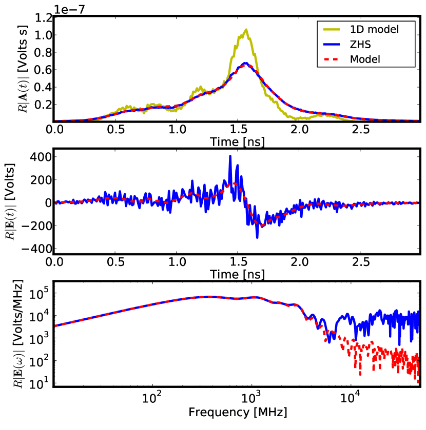
Figure 3: Results of the ZHS Monte Carlo compared to our calculation Eq. (17) for the radiation due to a $3\times 10^{18}$ eV electromagnetic shower observed at $\theta=\theta_{C}-0.3^{\circ}$ in the far-field in ice. The method is applied to the charge excess longitudinal profile obtained from the same simulation. Top panel: Vector potential in the time-domain with 10 ps time sampling (corresponding to a sampling frequency of 100 GHz) as obtained in ZHS simulations. This is compared to the calculation presented in this work. The longitudinal charge profile is shown as the 1D model presented in ARZ10 where the depth and charge are linearly rescaled to give the observer time and vector potential. Middle panel: Electric field in the time-domain comparing our method to ZHS results. Bottom panel: The electric field amplitude spectrum obtained from the ZHS simulation and the Fourier transform amplitudes of the electric field obtained from the calculation presented in this work. Note that the discrepancy between the time-domain electric field of the ZHS simulations and our results are due to the incoherent radiation at high frequencies.

In Fig. 3 we show an example of the vector potential and electric field in the time-domain due to an electromagnetic shower with energy $E=100$ EeV from the ZHS simulation. The fields are observed in the Fraunhofer region at an angle $\theta=\theta_{C}-0.3^{\circ}$ and they are compared to our results obtained with Eq. (17) using the longitudinal distribution $Q(z^{\prime})$ from the same simulation. The agreement between the vector potential obtained directly in the Monte Carlo simulation and the prediction of Eq. (17) lies within a few percent difference in the region relevant to the pulse (top panel of Fig. 3). The difference between this calculation and the ZHS electric field in the time domain is greater (middle panel of Fig. 3), but as shown in the bottom of Fig. 3 this is due mostly to the incoherent emission of the shower at high frequencies. The Fourier-transformed amplitudes of the time-domain electric field obtained in our approach are based on smooth parameterizations, while the frequency spectrum obtained directly in the ZHS simulation includes incoherence effects coming from the fine structure of the shower at the individual particle level.

Note that when $f(r^{\prime},z^{\prime})=\delta(r^{\prime})/r^{\prime}$, i.e. if we neglect the lateral distribution of the shower, Eq. (17) reduces to the 1-dimensional model in ARZ10 which fails at describing the features of the radio emission for angles close to the Cherenkov angle. To illustrate this, we show in the top panel of Fig. 3 the vector potential obtained in the one dimensional (1D) model in ARZ10 , which is a linear rescaling of the longitudinal charge excess profile, showing a clear disagreement with the results of the full ZHS simulation as expected.

II.3 Askaryan pulses in the “near-field”

We can now generalize Eq. (17) for an observer in the “near-field” region of the shower. In this case it is more natural to work in cylindrical coordinates and place the observer at $(r\cos\phi,r\sin\phi,z)$. Without loss of generality we can again assume the observer is at $\phi=0$ giving

$$|\mathbf{x}-\mathbf{x}^{\prime}|=\sqrt{r^{2}+r^{\prime 2}-2rr^{\prime}\cos\phi^{\prime}+(z-z^{\prime})^{2}}.$$ (18)

In dense media, the lateral distribution is in the scale of centimeters, which means that for all practical purposes the observer is at any given instant in the far-field region with respect to the lateral distribution. The idea is to solve the vector potential in Eq. (4) using the Fraunhofer approximation to account for the lateral distribution at any given time $t^{\prime}$. We expand Eq. (18) to first order in $r^{\prime}$ giving

$$|\mathbf{x}-\mathbf{x}^{\prime}|=\sqrt{r^{2}+(z-z^{\prime})^{2}}-r^{\prime}\sin\theta(z^{\prime})\cos\phi^{\prime}.$$ (19)

where $\sin\theta(z^{\prime})=r/\sqrt{r^{2}+(z-z^{\prime})^{2}}$, but we take into account that the distance in the denominator of the vector potential depends on the time $t^{\prime}$ or equivalently on the position $z^{\prime}$ in the shower as $\sqrt{r^{2}+(z-z^{\prime})^{2}}$. This is in contrast to the case of the far field calculation in which the distance in the denominator of the vector potential is constant and equal to $R$.

We proceed as in the case of the far-field calculation assuming that $f(r^{\prime},z^{\prime})\simeq f(r^{\prime})$ and $\mathbf{v}(r^{\prime},\phi^{\prime},z^{\prime})\simeq\mathbf{v}(r^{\prime},\phi^{\prime})$. After integrating over $t^{\prime}$ the vector potential in Eq. (4) can be written as,

$$\begin{split}&\mathbf{A}(r,z,t)=\frac{\mu}{4\pi}\int_{-\infty}^{\infty}dz^{\prime}\frac{Q(z^{\prime})}{\sqrt{r^{2}+(z-z^{\prime})^{2}}}\\ &\int_{-\infty}^{\infty}dr^{\prime}r^{\prime}\int_{0}^{2\pi}d\phi^{\prime}f(r^{\prime})~{}\frac{\mathbf{v}_{\perp}(r^{\prime},\phi^{\prime},z^{\prime})}{v}\\ &\delta\left(\frac{z^{\prime}}{v}+\frac{n\sqrt{r^{2}+(z-z^{\prime})^{2}}-nr^{\prime}\sin\theta(z^{\prime})\cos\phi^{\prime}}{c}-t\right)\end{split}$$ (20)

where the transverse projection of the velocity vector $\mathbf{v}_{\perp}(r^{\prime},\phi^{\prime},z^{\prime})=-\mathbf{\hat{u}}(z^{\prime})\times[\mathbf{\hat{u}}(z^{\prime})\times\mathbf{v}(r^{\prime},\phi^{\prime})]$ now introduces a new dependence on the longitudinal source coordinate $z^{\prime}$ due to the fact that in the near-field $\mathbf{\hat{u}}(z^{\prime})=(\mathbf{r}+(z-z^{\prime})\mathbf{\hat{z}})/\sqrt{r^{2}+(z-z^{\prime})^{2}}$ depends on $z^{\prime}$. If we define the form factor containing the radial $r^{\prime}$ and azimuthal $\phi^{\prime}$ integrals as in subsection II.A we obtain a similar expression:

$$\begin{split}&{\mathbf{F}}\left(t-\frac{z^{\prime}}{v}-\frac{n\sqrt{r^{2}+(z-z^{\prime})^{2}}}{c}\right)=\\ &\int_{-\infty}^{\infty}dr^{\prime}r^{\prime}\int_{0}^{2\pi}d\phi^{\prime}~{}f(r^{\prime})~{}\frac{\mathbf{v}_{\perp}(r^{\prime},\phi^{\prime},z^{\prime})}{v}\\ &\delta\left(\frac{z^{\prime}}{v}+\frac{n\sqrt{r^{2}+(z-z^{\prime})^{2}}}{c}-t-\frac{nr^{\prime}\sin\theta(z^{\prime})\cos\phi^{\prime}}{c}\right)\end{split}$$ (21)

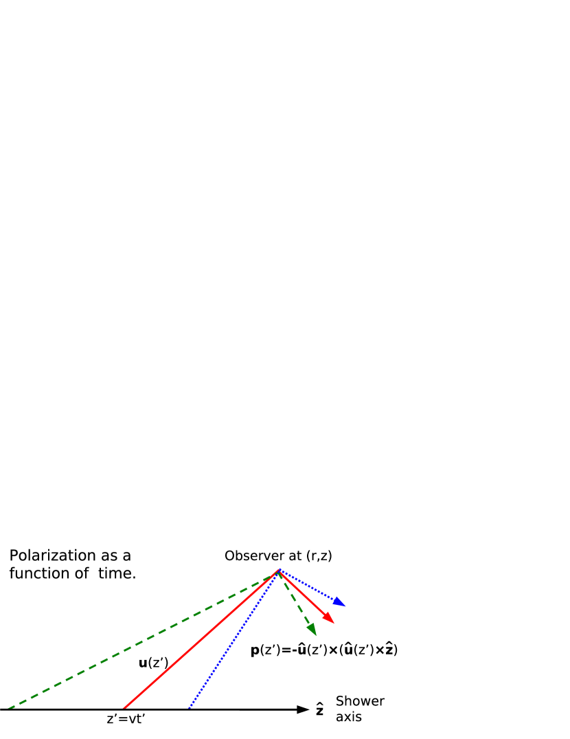
Figure 4: Sketch illustrating the polarization dependence with time. As the shower evolves the observer sees the radiation contributions at different angles corresponding to different source positions $z^{\prime}$. This means that the observer will see the polarization vector changing as a function of time $t$.

Note that the form factor defined in Eq. (21) has the same functional form as that defined in Eq. (15) and they only differ in the argument of the delta function. The form factor $\mathbf{F}$ as obtained in the far field can be applied to the near field (in relation to the longitudinal development of the shower) simply modifying its argument.

Neglecting again the component of $\mathbf{F}$ parallel to $\mathbf{\hat{u}}$ the vector potential in the near-field can be written as:

$$\begin{split}&\mathbf{A}(r,z,t)=\frac{\mu}{4\pi}\int_{-\infty}^{\infty}dz^{\prime}\frac{Q(z^{\prime})}{\sqrt{r^{2}+(z-z^{\prime})^{2}}}~{}\mathbf{p}(z^{\prime})\\ &F_{p}\left(t-\frac{z^{\prime}}{v}-\frac{n\sqrt{r^{2}+(z-z^{\prime})^{2}}}{c}\right)\end{split}$$ (22)

Note that a new $z^{\prime}$ dependence is introduced through the polarization vector $\mathbf{p}(z^{\prime})=-\mathbf{\hat{u}}(z^{\prime})\times(\mathbf{\hat{u}}(z^{\prime})\times\mathbf{\hat{z}})$. In Fig. 4 an example is shown of the $z^{\prime}$ dependence of $\mathbf{p}(z^{\prime})$. Also note that the $\sin\theta$ term in Eq. (17) has been absorbed in Eq. (22) through $\mathbf{p}=\sin\theta~{}\mathbf{\hat{p}}$

In the near field the explicit $z^{\prime}$ dependence is necessary because the longitudinal profile of the shower is observed at different angles. This means that parts of the shower observed at different depths will have differing polarization vectors. This modification accounts exactly for the interference between different $z^{\prime}$ points along the shower development. This result has also been determined from a one dimensional current density model in Chen_ARENA_2010 .

Eq. (22) tells us that the vector potential in the near-field region of the shower can be obtained as a convolution of the form factor $F_{p}$ - that parameterizes the interference effects due to the lateral distribution of the shower - and the longitudinal profile of the excess charge. The form factor function $F_{p}$ has to be evaluated at the time $t$ at which an observer in the near field sees the portion of the shower corresponding to the depth $z^{\prime}$. That time is clearly given by $t=z^{\prime}/v+n\sqrt{r^{2}+(z-z^{\prime})^{2}}/c$. The difference between this expression and that obtained in the far field is that $F_{p}$ is always evaluated at the time $t$ an observer sees the position $z^{\prime}$ in the shower which is different for the far- and near-field regions.

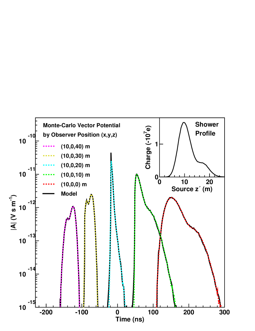
Figure 5: The Fresnel region vector potential for an electron induced $100$ PeV shower in ice from the ZHS Monte Carlo compared to the results of Eq. (22). The longitudinal profile of the excess charge is convolved with the form factor $F_{p}$. The observers are located at $(x,y,z)$ where $z$ lies along the shower axis and $y=0$. The vector potentials have been arbitrarily shifted in time by multiples of 50 ns for clarity. The spiked vector potential in the middle (blue) corresponds to an observation where the peak of the longitudinal shower profile is near the Cherenkov angle. The vector potentials to the right of it (green and red) are due to observations above the Cherenkov angle while the vector potentials to the left (magenta and yellow) are due to observations below the Cherenkov angle. Note the inverted order of the primary and secondary peaks.

In Fig. 5 we show an example of the vector potential in the time domain for various observers in the near field region of the shower as obtained in full ZHS simulations. The shower has an energy $E=100$ PeV and a longitudinal dimension of $\sim 25$ m, and the observer is placed at different positions $z$ along the shower axis and at a fixed radial distance $r=10$ m. The ZHS simulation also gives the longitudinal profile of the excess charge $Q(z^{\prime})$ which we have introduced into Eq. (22) to obtain the vector potential and compare it to that obtained directly by the Monte Carlo, also shown in Fig. 5. The agreement between the vector potential obtained directly in the Monte Carlo simulation and the calculation in our approach is remarkable. For distances to the shower axis larger than $\sim 1~{}{\rm m}$ the difference between our approach and the Monte Carlo is typically $\sim 1~{}\%$ or better for values down to $\sim 3$ orders of magnitude below the peak of the vector potential. This difference starts to increase gradually as the distance to the shower axis decreases and becomes comparable to the lateral dimensions of the shower, where the parameterization of the vector potential at the Cherenkov angle given in Eq. (16) is not expected to be valid. Since the typical distance between antennas in experiments such as the Askaryan Radio Array (ARA) ARA is $\sim 10-100$ m, we expect our results to be accurate enough in most practical situations.

III The apparent motion of a charge distribution.

The temporal behavior of the vector potential traces the motion of a charged particle according to the retarded time. This is an old idea discussed by Feynman in Feynman1963 applied to elucidate on the properties of synchrotron radiation. More recently, this approach has also been used in the Cherenkov radiation calculation due to linear tracks in the near field Afanasiev_book and one dimensional current densities in Chen_ARENA_2010 . In this section we analyze the characteristics of our results in terms of the apparent motion of the charge density distribution to gain an intuitive understanding of the radiation due to a particle shower developing in a homogeneous dielectric medium.

III.1 Time delay effects

The apparent motion of particles is encoded in the Green’s function solution of the vector potential, Eq. (4), by the argument of the delta function taking the source time $t^{\prime}$ to the observer time $t$:

$$t=t^{\prime}+\frac{n|\mathbf{x}-\mathbf{x}^{\prime}|}{c}$$ (23)

The term $|\mathbf{x}-\mathbf{x}^{\prime}|$ traces the motion of the current density vector $\mathbf{J}$ at position $\mathbf{x}^{\prime}(t^{\prime})$ to determine the observer time.

We can gain much insight into the properties of the vector potential resulting from the ZHS particle shower simulation, shown in Fig. 5, by momentarily ignoring the lateral distribution of the shower. In this case the observer time $t$ is given in terms of the source time $t^{\prime}$ by

$$t=t^{\prime}+\frac{n\sqrt{r^{2}+(z-vt^{\prime})^{2}}}{c}$$ (24)

where we have substituted $z^{\prime}=vt^{\prime}$ and $r$ is the cylindrical radial position of the observer.

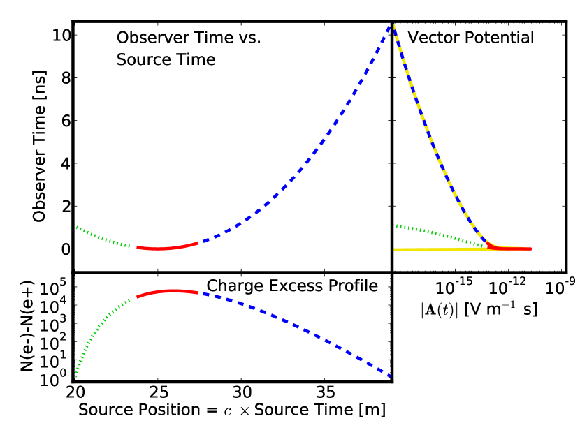
Figure 6: Illustration of the vector potential characteristics due to the apparent motion of the charge distribution for an observer seeing the region around shower maximum with angles close to the Cherenkov angle in ice ($n=1.78$). In the bottom plot we show the longitudinal charge excess profile following a Greisen parameterization. The center plot shows the observer time as a function of the source time for a shower exceeding the speed of light in a medium. The solid (red) portion, corresponding to the minimum of the source and observer time relation, contributes significantly to the radiation near the Cherenkov peak. The resulting vector potential is shown in the right hand side. The Cherenkov radiation spike corresponds to the compressed mapping of the charge excess distribution to the observer time.

When $v<c/n$, Eq. (24) has a unique observer time corresponding to each source time. However, in the case of $v>c/n$ there always exist a range of observer positions such that Eq. (24) has two source times corresponding to every observer time (see an example in the top left panel of Fig. 6). In addition, a minimum value of $t$ (different from the trivial minimum $z^{\prime}_{0}$ corresponding the beginning of the shower at $t^{\prime}_{0}$) may exist when $n\beta>1$. In other words, the observer first sees the radiation corresponding to a depth in the shower $z^{\prime}_{\mbox{\footnotesize{min}}}\neq z^{\prime}_{0}$ and then sees contributions from shower depths before and after arriving simultaneously. This minimum can be characterized by looking at the derivative of the retarded time relation,

$$\frac{\partial t}{\partial t^{\prime}}=1-n\beta\frac{z-vt^{\prime}}{\sqrt{r^{2}+(z-vt^{\prime})^{2}}}$$ (25)

The extrema in the relation between the source time and the observer time are given by requiring the above equation to be equal to zero. A solution exists only when $v>c/n$ and indeed corresponds to a minimum value in the observer time $t_{\mbox{\footnotesize{min}}}$. The corresponding shower coordinate $z^{\prime}_{\mbox{\footnotesize{min}}}$ given by the source time $t^{\prime}_{\mbox{\footnotesize{min}}}=z^{\prime}_{\mbox{\footnotesize{min}}}/v$ is

$$z^{\prime}_{\mbox{\footnotesize{min}}}=z+\frac{r}{\sqrt{n^{2}\beta^{2}-1}}.$$ (26)

The angle of observation $\theta$ with respect to the shower axis corresponding to the shower position $z^{\prime}$ is given by:

$$\cos\theta=\frac{(z-z^{\prime})}{\sqrt{r^{2}+(z-z^{\prime})^{2}}}$$ (27)

when $z^{\prime}=z^{\prime}_{\mbox{\footnotesize{min}}}$ it is straightforward to show that the angle corresponds to the Cherenkov angle $\cos\theta_{C}=1/(n\beta)$, i.e. the minimum time $t_{\mbox{\footnotesize{min}}}$ at which the observer first sees the shower corresponds to the shower coordinate lying at the Cherenkov angle. Its value is given by

$$t_{\mbox{\footnotesize{min}}}=\frac{z}{v}+\frac{r\sqrt{n^{2}\beta^{2}-1}}{v}$$ (28)

A peculiar consequence of these relations is that if an observer is placed at a position such that the shower is always seen with $\theta<\theta_{C}$ then $z^{\prime}_{\rm min}$ corresponds to the end of the shower, which is an apparent violation of causality. In the case where $\theta>\theta_{C}$ then $z^{\prime}_{\rm min}$ corresponds to the beginning of the shower as expected. This relation can be seen in Fig. 7 and is discussed in depth later in this section.

In the analytical solution (Fig. 6), for that particular observer seeing the region around shower maximum with angles close to the Cherenkov angle, it is evident that a given observation time $t$ corresponds to two different shower coordinates $z^{\prime}_{\pm}$ one corresponding to an early development of the shower observed at angle $\theta<\theta_{C}$ and the other to a late one at angle $\theta>\theta_{C}$. When viewing particle showers around the Cherenkov angle in the near-field, the radiation due to the early parts of the shower interferes with radiation due to the late parts of the shower. The apparent violation of causality is a relativistic effect due to the index of refraction of the medium being $n>1$. Note also that for shower positions observed below the Cherenkov angle the derivative $\partial t/\partial t^{\prime}<0$ meaning that time appears to run backwards.

The depths $z^{\prime}_{\pm}$ are easily obtained by expressing the source time $t^{\prime}$ in terms of the observer time $t$ by inverting Eq. (24):

$$t^{\prime}_{\pm}=\frac{z^{\prime}_{\pm}}{v}=\frac{vz-c^{2}_{n}t}{(v^{2}-c_{n}^{2})}\pm c_{n}\frac{\sqrt{(z-vt)^{2}-r^{2}(n^{2}\beta^{2}-1)}}{(v^{2}-c_{n}^{2})}$$ (29)

where $c_{n}=c/n$. Real solutions exist if the argument of the square root is non-negative which is equivalent to $t>t_{\mbox{\footnotesize{min}}}$ with $t_{\mbox{\footnotesize{min}}}$ given in Eq. (28).

The features of the vector potential due to the apparent motion of a charge distribution along an axis with $v>c/n$ are illustrated in Fig. 6. In the bottom panel we show the Greisen parametrized longitudinal profile of the excess charge as a function of $z^{\prime}$ or equivalently $t^{\prime}$. In the center panel we show the relation between $t$ and $t^{\prime}$ given in Eq. (24) for ice ($n=1.78)$ with the shower front traveling at the speed of light. This relation has a minimum at $t^{\prime}_{\mbox{\footnotesize{min}}}=z^{\prime}_{\mbox{\footnotesize{min}}}/v$ given in Eq. (26) which corresponds to an observer time $t_{\mbox{\footnotesize{min}}}$ given in Eq. (28). Around $t^{\prime}_{\mbox{\footnotesize{min}}}$ the derivative $\partial t/\partial t^{\prime}$ is very small and as a consequence the charge density of the source that corresponds to a relatively wide interval of source times $t^{\prime}_{\mbox{\footnotesize{min}}}\pm\Delta t^{\prime}=t^{\prime}_{\mbox{\footnotesize{min}}}\pm\Delta z^{\prime}/v$, is projected and seen by the observer during a small interval $t_{\mbox{\footnotesize{min}}}\pm\Delta t$ where,

$$\frac{\Delta t}{\Delta t^{\prime}}=\frac{\partial t}{\partial t^{\prime}}$$ (30)

This causes a time compression which enhances the radiation, especially when the geometry is such that at $t_{\mbox{\footnotesize{min}}}$ the observer located at $(r,0,z)$ sees the region around the shower maximum. This is illustrated in the right panel of Fig. 6 where the vector potential corresponding to the charge distribution shown in the bottom panel is depicted. The sharp initial peak of the vector potential is due to the compression of radiation into a short interval of time as seen by the observer. For late enough observer times, the relation between the apparent and the observer time approaches linearity and the relation is causal. The observer sees later parts of the shower, shown in the bottom panel of Fig. 6, at later times. This corresponds to the long tail in the vector potential depicted in the right panel of Fig. 6. It is worth remarking that the relativistic effects described here arise in any situation where $v>c/n$ and are not limited to the description of Askaryan radiation zhaires_air11 .

III.2 Interpretation of simulation results

The corresponding time delay analysis of the results of the ZHS particle simulation shown in Fig. 5 is displayed in Fig. 7, using the same profile and source positions as depicted in Fig. 5. The observer located at $(x,y,z)=(10,0,20)$ m in Figs. 5 and 7, sees a sharp and strong spike in the vector potential (and electric field) that is not matched by that seen by observers located at other positions in Fig. 5. In the middle panel of Fig. 7 we show the corresponding observer time $t$ vs. the source position $z^{\prime}$ relation. For the observer at $(10,0,20)$ m one can clearly see a region with a small derivative $\partial t/\partial t^{\prime}$ responsible for the compression effect which leads to an enhancement in the vector potential. As shown with the aid of Eq. (27) the time at which an observer sees the shower first corresponds to observation at the Cherenkov angle. This can be also seen in the top panel of Fig. 7 where we have plotted the angle between the position $z^{\prime}$ along the shower axis and the location of the observer. An observer at $(10,0,10)$ m also sees a fraction of the shower with angles around the Cherenkov angle. The Cherenkov pulse is not as pronounced because the net charge in that region is significantly smaller than the charge at shower maximum, and does not last as long as what the observer at $(10,0,20)$ m sees. In this view Cherenkov radiation is a geometrical phenomenon due to the minimum in the relation between the observer time and the source position.

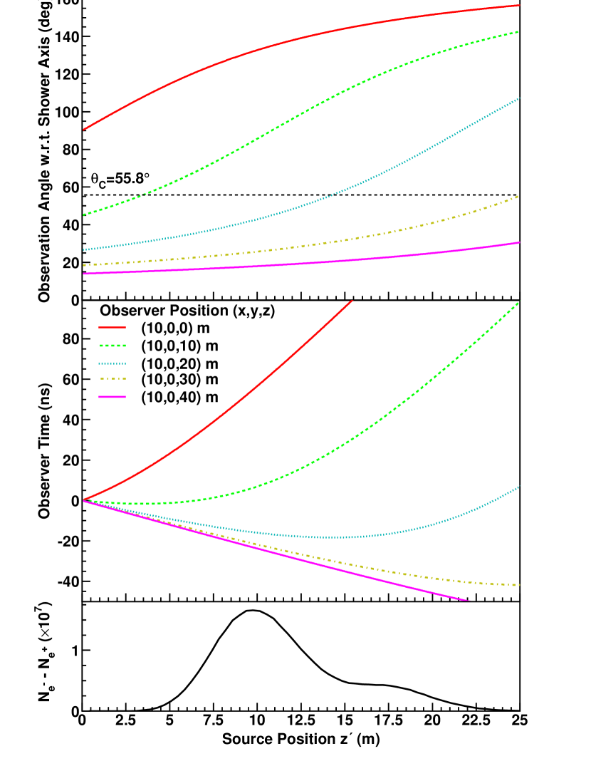
Figure 7: Apparent motion analysis of the charge distribution for the vector potentials shown in Fig. 5. Bottom panel: Longitudinal profile of the excess negative charge in the 100 PeV electron-induced shower. Middle panel: Observer time $t$ vs source position $z^{\prime}$ for the same observers as in Fig 5. Top panel: Angle with which each observer sees the different positions $z^{\prime}$ in the shower axis. The Cherenkov angle ($\theta_{C}=55.8^{\circ}$ in ice) is indicated with a long-dashed horizontal line. See text for a description of the mapping of these relations to the features of the vector potentials shown in Fig. 5.

The apparent causality violations are manifested in the shape of the vector potential as viewed by different observers. An observer at an angle smaller than the Cherenkov angle will see the evolution of the shower with an inverted causal order at all times. This is the case of the vector potential labeled $(x,y,z)=(10,0,40)$ m in Fig. 5 where the observer sees a $\sim 25$ m long 100 PeV energy shower (shown in the inset of Fig. 5 and in the bottom of Fig. 7) with the radiation corresponding to larger depths at later times. The longitudinal charge excess distribution shown in Fig. 7 has a primary peak followed by a smaller secondary peak. The vector potential traces this feature but in the reversed time sequence. In the case of an observation at angles larger than $\theta_{C}$, the shower is seen in the normal causal order at all times. This case is illustrated by vector potential labeled $(x,y,z)=(10,0,10)$ m in Fig. 5 where the radiation corresponding to the charge excess distribution at larger depths is observed at later times. The peaks of the vector potential match the order of the peaks of the charge excess distribution in the bottom of Fig. 7. It is also worth noting that even though single antenna measurements in the near-field make it difficult to reconstruct the longitudinal profile of the charge excess, observations from multiple stations located at tens of meters from the shower axis, do provide the necessary information.

IV Summary and Outlook

We have derived a highly detailed and computationally efficient approach for the calculation of Askaryan pulses. The electrodynamic calculations leading to the relation between the pulse features and the shower characteristics can be intuitively understood via the apparent motion of charges. Viewed from this perspective, one can easily retrace the time-domain behavior of the pulse to the shape of the electromagnetic shower and the observer versus source time relation as shown in Fig. 6.

There are many interesting features of Askaryan radiation due to the fact that the speed of the shower front exceeds the speed of light. In this treatment, the radiation due to the charge excess of an electromagnetic shower is understood as a “dense” or compressed mapping of the charge excess profile to the vector potential via the observer vs. source time relation. The mapping is densest at the minimum of the observer vs. source time relation which corresponds to observations at the Cherenkov angle. In addition, for observation at angles smaller than the Cherenkov angle, time appears to run backwards. This manifests itself in the time-reversed mapping of the longitudinal profile of the charge excess to the time-domain vector potential.

The primary motivation for developing this calculation in the time-domain is to understand the temporal behavior of the Askaryan pulse. In the frequency domain, this is equivalent to understanding the phase versus frequency relation. Although it is possible to do this in a completely frequency-domain approach, the time-domain relations can be intuitively understood and are easier to compute.

The computational algorithm presented here is summarized as follows:

1. Compute the vector potential of the Askaryan pulse at the Cherenkov angle $\mathbf{A}(\theta_{C},t)$ and use it together with total charged track-length $LQ_{tot}=\int dz^{\prime}Q(z^{\prime})$ to extract the functional form of the form factor $F_{p}$. (This has been done in this article for electromagnetic showers in ice and in that case it is possible to use directly the parameterization provided in Eq. (16). For other situations it needs to be re-evaluated with a detailed Monte Carlo simulation.)

2. Obtain the charge excess longitudinal profile of an electromagnetic shower $Q(z^{\prime})$. This can be provided as either the output of a particle shower simulation or using a parameterization.

3. Convolve $F_{p}$ with $Q(z^{\prime})$ according to Eq. (17) in the far-field or Eq. (22) in the near-field to obtain the time-domain vector potential.

4. Electric fields are obtained from a trivial numerical derivative of the vector potential with respect to time: ${\mathbf{E}}=-\partial{\mathbf{A}}/\partial t$.

The formalism developed here can also be applied to the reconstruction of longitudinal shower profiles. In the far-field this can only be done if the pulse was detected away from the Cherenkov angle, otherwise the pulse shape is approximately the same for any given longitudinal charge excess profile. Away from the Cherenkov angle the pulse traces the shape of the longitudinal profile convolved with the lateral profile response. For very extended longitudinal profiles, such as those resulting from UHE showers affected by the LPM effect, the tracing of the profile can be seen for angles as small as $0.3^{\circ}$ away from the Cherenkov angle (see Fig. 3). The overall quality of the reconstruction can be assessed with simulations that are specific to the experiment in question. The reconstruction of longitudinal profiles has interesting experimental applications such as the identification of the primary particle or $\nu$ flavor inducing the shower. This is particularly relevant for the electromagnetic component of a $\nu_{e}$-induced shower with its multiply-peaked structure due to the LPM effect.

In the near-field the reconstruction of shower longitudinal profiles is also possible. If the radiation is detected by a single station the reconstruction is complicated by the fact that the portions of the shower above and below the Cherenkov angle may interfere with each other depending on the position of the antenna. However, if multiple antennas observe the radiation due to a single shower it is possible to obtain a highly constrained reconstruction of the longitudinal profile. The example depicted in Fig. 5 shows a case where this could be done for antennas in ice spaced tens of meters apart. The formalism provided in this paper will allow the experimentalist to simulate these measurements and find the optimal antenna placement and assess the quality of reconstruction. This would be of particular interest to an array such as the future planned ARA ARA and ARIANNA ARIANNA experiments where the shower could potentially be observed by multiple stations in Antarctic ice.

In a future publication we plan to produce time-domain parameterizations of the vector potential at the Cherenkov angle for electromagnetic showers in various media such as salt and the lunar regolith. In addition the time-domain parameterizations of hadronic showers will be included which will allow the experimentalist to produce full simulations of neutrino interactions with flavor dependent parameters. This will be useful for experiment simulations and candidate event reconstructions.

V Acknowledgments

J.A-M and E.Z. thank Xunta de Galicia (INCITE09 206 336 PR) and Consellería de Educación (Grupos de Referencia Competitivos – Consolider Xunta de Galicia 2006/51); Ministerio de Ciencia e Innovación (FPA 2007-65114, FPA 2008-01177 and Consolider CPAN - Ingenio 2010) and Feder Funds, Spain. We thank CESGA (Centro de SuperComputación de Galicia) for computing resources and assistance. A.R-W thanks NASA (NESSF Grant NNX07AO05H). Part of this research was carried out at the Jet Propulsion Laboratory, California Institute of Technology, under a contract with the National Aeronautics and Space Administration. We thank J. Bray, P. Gorham, C.W. James and W.R. Carvalho Jr. for helpful discussions.

References

- (1) Askar’yan, G.A., Soviet Physics JETP 14,2 441–443 (1962); 48 988–990 (1965).
- (2) D. Saltzberg et al., Phys. Rev. Lett. 86, 2802 (2001).
- (3) P. Miocinovic et al. Phys. Rev. D 74, 043002 (2006).
- (4) P.W. Gorham et al. Phys. Rev. D 72, 023002 (2005).
- (5) P.W. Gorham et al. Phys. Rev. Lett. 99, 171101 (2007).
- (6) T. Hankins et al. Mon. Not. Royal Astron. Soc. 283, 1027 (1996);
- (7) I. Kravchenko et al., Astropart. Phys. 19, 15 (2003); I. Kravchenko et al., Phys. Rev. D 73, 082002 (2006).
- (8) P.W. Gorham et al. Phys. Rev. Lett. 93, 041101 (2004).
- (9) O. Scholten et al. Astropart. Phys. 26, 219 (2006).
- (10) A.R. Beresnyak et al. Astronomy Reports 49 2, 127 (2005).
- (11) P.W. Gorham et al. Phys. Rev. Lett. 103, 051103 (2009).
- (12) C.W. James et al. Phys. Rev. D 81, 042003 (2010).
- (13) T.R. Jaeger, R.L. Mutel, K.G. Gayley, Astropart. Phys. 34, 293 (2010).
- (14) P. Allison et al. [The ARA Collaboration], arXiv:1105.2854 [astro-ph]. The ARA Collaboration: ARA proposal. “Instrument Development of the Askar´yan Radio Array, a Large-scale Radio Cherenkov Detector at the South Pole”, available at: http://grid.ntu.edu.tw/html/projects/pro101/pro101.pdf
- (15) S.W. Barwick et al. J. Phys. Conf. Ser. 60, 276-286 (2007).
- (16) F. Halzen, E. Zas, T. Stanev, Phys. Lett. B 257, 432 (1991).
- (17) E. Zas, F. Halzen, T. Stanev, Phys. Rev. D 45, 362 (1992).
- (18) J. Alvarez-Muñiz, E. Zas, Phys. Lett. B 411, 218 (1997).
- (19) J. Alvarez-Muñiz, E. Zas, Phys. Lett. B 434, 396 (1998).
- (20) J. Alvarez-Muñiz, R.A. Vázquez and E. Zas, Phys. Rev. D 61, 023001 (1999).
- (21) J. Alvarez-Muñiz, R.A. Vázquez, E. Zas, Phys. Rev. D 62, 063001 (2000).
- (22) S. Razzaque et al. Phys. Rev. D 65, 103002 (2002);
- (23) J. Alvarez-Muñiz, E. Marqués, R.A. Vázquez, E. Zas, Phys. Rev. D 67, 101303 (2003).
- (24) S. Razzaque et al. Phys. Rev. D 69, 047101 (2004).
- (25) S. Hussain, D.W. McKay, Phys. Rev. D 70, 103003 (2004).
- (26) J. Alvarez-Muñiz, E. Marqués, R.A. Vázquez, E. Zas, Phys. Rev. D 74, 023007 (2006).
- (27) J. Alvarez-Muñiz, C.W. James, R.J. Protheroe and E. Zas, Astropart. Phys. 32, 100 (2009).
- (28) J. Alvarez-Muñiz, W. Rodrigues, M. Tueros and E. Zas, arXiv:1005.0552 [astro-ph].
- (29) J. Alvarez-Muñiz, A. Romero-Wolf, E. Zas, Phys. Rev. D 81, 123009 (2010).
- (30) M. DuVernois, B. Cai, D. Kleckner, in: Proceedings of the 29th ICRC, Pune, India, 2005, p. 311.
- (31) A.A. Konstantinov, Ph.D. Thesis, Lomonosov Moscow State University (2009).
- (32) M. Ludwig, T. Huege, Astropart. Phys. 34, 438 (2011).
- (33) V. Marin, R. Dallier, Proc. of the ARENA 2010 meeting, Nantes, France (2010), Nucl. Instr. Meth. Phys. Res. A in press.
- (34) J. Alvarez-Muñiz, W.R. Carvalho, E. Zas, A. Romero-Wolf, M. Tueros, Procs. of the ARENA 2010 meeting, Nantes, France (2010), Nucl. Instr. Meth. Phys. Res. A in press;
- (35) J. Alvarez-Muñiz, W.R. Carvalho, E. Zas, arXiv:1107.1189 [astro-ph].
- (36) C.-Y. Hu, C.-C. Chen, P. Chen, arXiv:1012.5155
- (37) A. Taflove, S.C. Hangess, “Computational Electrodynamics: The Finite-Difference Time-Domain Method” (Artech House, London, 2005).
- (38) R.V. Buniy, J.P. Ralston, Phys. Rev. D 65, 016003 (2002).
- (39) L. Landau, I. Pomeranchuk, Dokl. Akad. Nauk SSSR 92, 535 (1953); 92, 735 (1935); A.B. Migdal, Phys. Rev. 103, 1811 (1956); Zh. Eksp. Teor. Fiz. 32, 633 (1957) [Sov. Phys. JETP 5, 527 (1957)].
- (40) T. Stanev et al., Phys. Rev. D 25, 1291 (1982).
- (41) T. Huege, H. Falcke, Astron. & Astrophys. 412, 19 (2003).
- (42) O. Scholten, K. Werner, R. Rusydi, Astropart. Phys. 29, 94 (2008).
- (43) N. Meyer-Vernet, A. Lecacheaux, D. Ardouin, Astron. & Astrophys. 480, 15 (2008)
- (44) J. Chauvin et al., Astropart. Phys. 33, 341 (2010).
- (45) O. Scholten, K. Werner, Astropart. Phys. 29, 393 (2008).
- (46) J. Alvarez-Muñiz, W.R. Carvalho, D. García-Fernández, A. Romero-Wolf, E.Zas in preparation (2011).
- (47) J.D. Jackson, Am. J. Phys. 70 (9), 917 (2002).
- (48) J.D. Jackson, Classical Electrodynamics 3rd Ed. Wiley, New York, (1998).
- (49) K. Greisen, Annual Reviews of Nuclear Science 10, 63 (1960)
-
(50)
C. Chen, Presentation in ARENA 2010. Link: http://indico.in2p3.fr/contributionDisplay.py?sessionId=4&
contribId=45&confId=2719 - (51) R.P. Feynman, R.B. Leighton, M. Sands, The Feynman Lectures in Physics. Addison-Wesley, (1963).
- (52) G.N. Afanasiev, Vavilov-Cherenkov and synchrotron radiation: foundations and applications, Kluwer Academic Publishers, (2004)